Land Cover Mapping with Higher Order Graph-Based Co-Occurrence Model

Abstract

Deep learning has become a standard processing procedure in land cover mapping for remote sensing images. Instead of relying on hand-crafted features, deep learning algorithms, such as Convolutional Neural Networks (CNN) can automatically generate effective feature representations, in order to recognize objects with complex image patterns. However, the rich spatial information still remains unexploited, since most of the deep learning algorithms only focus on small image patches that overlook the contextual information at larger scales. To utilize these contextual information and improve the classification performance for high-resolution imagery, we propose a graph-based model in order to capture the contextual information over semantic segments of the image. First, we explore semantic segments which build on the top of deep features and obtain the initial classification result. Then, we further improve the initial classification results with a higher-order co-occurrence model by extending the existing conditional random field (HCO-CRF) algorithm. Compared to the pixel- and object-based CNN methods, the proposed model achieved better performance in terms of classification accuracy.

1. Introduction

Remote sensing images can provide inexpensive, fine-scale information with multi-temporal coverage which has proven to be useful in terms of urban planning, land-cover mapping, and environmental monitoring. To enable high-resolution satellite image interpretation, it is important to label image pixels with their semantic classes. Intensive studies have been conducted in high-resolution image classification and labeling [1,2,3]. Pixel-based image classification methods were initially developed to label each pixel for the entire image, with methods such as the maximum likelihood classifiers (MLC) or support vector machine (SVM). In order to obtain more accurate classification results, it is common to apply representative feature extraction techniques (such as gray-level co-occurrence matrix (GLCM) [4] or morphological attribute profiles (MAPs) [5,6]) as standard preprocessing steps. However, due to the variability in high-resolution images, it is difficult to find robust and representative feature representations for efficient image classification [7,8]. In addition, the pixel-based classification methods suffer from the salt-and-pepper phenomenon, since they overlook the rich spatial information of the high-resolution images.

In order to utilize the rich spatial information and improve classification performance, object-based image classification methods [9,10] have been intensively investigated. Instead of directly classifying the whole image in a pixel-wise fashion, the object-based methods effectively interpret the complex high-resolution images in terms of image segments. More specifically, the object-based methods first split an image into several homogeneous objects and then infer the semantic label of each segment by applying a majority voting strategy. Thus, it overcomes the salt-and-pepper defect characteristic of pixel-based methods. However, it is difficult to accurately segment complex scenes into meaningful parts, due to the complexity of high-resolution remote sensing images. For example, building roofs are frequently segmented into shadowed areas, small objects (such as chimneys, windows) etc., Alternatively, graph-based random field methods have been used to interpret high-spatial resolution images by considering spatial interactions between neighboring pixels. As a representative, the Markov random fields (MRF) was first introduced as the graph-based image analysis method and has been successfully applied in remote sensing image classification [11,12]. But, the MRF is a generative model that only considers joint distributions in the label domain. To improve the performance of MRF, a technique known as conditional random fields (CRF) was proposed to directly model the posterior distribution by considering the joint distribution of both the label and observed data domain at the same time [13]. In other words, the potential functions in CRF-based algorithms are designed to measure the trade-off between spectral and spatial contextual cues. For instance, the support vector conditional random field classifier [14,15] was widely used to incorporate spatial information at the pixel-level which effectively overcomes the salt-and-pepper classification noise. Moreover, in order to improve the processing efficiency of high-resolution image classification, the object-based CRF model [16,17] was proposed and has successfully been used to classify images.

Although object- and graph-based image interpretation strategies have already been successfully applied in many applications, the challenges of accurate high-resolution image classification yet to be treated. There are two factors that heavily impact the traditional image classification accuracies: (1) The representations of complex geographical objects, (2) Contextual information utilization. For the first one, low-level feature descriptors often fail to represent complex geographical objects, due to the spectral variabilities of high-resolution images. For instance, building roofs in an urban area often contain antennas, chimneys, and shadows. Moreover, the traditional feature descriptors which only consider the spectral distribution, shape or texture of neighboring pixels and suffer from the variable nature of high-resolution imagery. Besides, the object- or graph-based models that built on heterogeneously low-level features are often too fragmented to depict accurate contours of complex geographical objects, let alone capture high-level contextual information. Therefore, we integrated the CNN-based deep features with low-level image segments, thus produce meaningful semantic segments which accurately capture geographical objects. In addition, we propose a graph-based class co-occurrence model in order to capture the rich contextual information in high-resolution images. More specifically, we investigated a convolutional neural network (CNN) with five layers to explore robust deep features which later have been used to generate semantic segments. Since geographical objects already can be accurately described by semantic segments, we further construct a semantic graph in order to get a better grasp of the contextual information in high-resolution images. Last but not least, we further proposed a higher-order co-occurrence CRF model (HCO-CRF) in addition to semantic segments in order to improve image classification accuracy.

The rest of paper is organized as follows: The related work such as CNN framework and the traditional CRF model is briefly introduced in Section 2. Then, the HCO-CRF model with considering class dependencies and label HCO-occurrences is presented in Section 3. In Section 4, the experimental setting, results, and analysis are illustrated. Finally, the conclusion is presented in Section 5.

2. Related Work

Previous studies have focused on the topic of semantic labeling of high-resolution remote sensing images. Specifically, on the exploration of deep learning algorithms, where some works refined the results based on contextual models in order to predict accurate labels. Here, we first review some of the previous studies that are related to our work.

2.1. Deep Convolutional Neural Networks

Recently, deep learning has made significant breakthroughs in terms of object recognition, image classification and semantic understanding of natural images. Also, due to the increasing availability of high-resolution remote sensing images, convolutional neural networks (CNNs) have been successfully applied to accurately classify remote sensing images. Unlike natural scene images, remotely acquired images are much more complicated, in terms of spectral or spatial patterns that represent geographical objects. In order to represent complex image patterns in a remote sensing image, CNNs build features from scratch in the first layer and then generate more representative features by merging, activating and regrouping former the original features. Some researches have focused on the exploration of CNNs with pixel-wise strategies, such as [18]. In these studies, CNNs performed as a classifier by using window sliding technique to figure out the class label of each pixel. For each pixel, a neighboring region with certain sizes can be directly fed into a CNN framework to produce deep features and predict labels. To boost the classification performance, several investigations extended the traditional CNNs by integrating prior knowledge, such as a hybrid framework and multi-scale strategy.

Following a different strategy, the fully convolutional neural networks (FCNNs) have been proposed to densely predict semantic labels in images. Compared to the traditional CNNs, the FCNNs overcome the effect of down-sampling during deep feature generation. It directly integrates abstract semantic information from deep, coarse layers with detailed shape contours from shallow layers in order to generate accurate semantic predictions. For the purpose of generating full-resolution feature maps, decode or deconvolutional layers can directly stretch low-resolution feature maps into the original input sizes [19,20]. Moreover, a well-trained CNN framework contains rich low-level contour information and high-level semantic features. To exploit the rich information, skip architectures have often been applied to combine coarse layer features with finer layer information in order to yield a more accurate classification, such as FCN-8s [21]. However, the utilization of FCNNs requires densely labeled training samples which is often impossible in most image classification tasks. The training samples (or reference data) for remote sensing image interpretation are scarce and difficult to acquire even with intense labor involvement. In this regard, the applications of FCNNs in the field of remote sensing classification are limited.

2.2. Graph-Based Context Model

In order to exploit contextual information in images, the graph-based methods have been intensively studied. For most graph-based methods, the energy functions are widely utilized in terms of contextual information formulation, such as MRFs and CRFs. The energy function serves as a smoother during the post-processing stage, it enforces the consistency of predicted labels in the classification map. Traditionally, the graph-based model considers label consistency at the pixel level and commonly with 4- or 8-neighboring pixels. However, due to the heterogeneity of high-resolution remote sensing images, pixel-based graph mode often failed to capture useful contextual information that lies in larger scales. Then, image segments were introduced to reduce the image heterogeneity and graph models can be built on the top of such segments. In this way, the graph is more meaningful and capturing contextual information more accurate than pixel-based fashion. Although, the graph model that builds on top of image segments can effectively capture more contextual information and reduce "salt and pepper" noises. Still, contextual information at larger scales remains unexploited. Recently, lots of works have been published in terms of higher-order graph models. One of the most popular methods is the integration of higher-order potential and graph cut algorithm to inference image classification results [22]. It captures contextual information at larger ranges, which is much richer than that in adjacent neighbors. The higher-order graph models are particularly suitable for remote sensing imagery interpretation since they formulate larger scale dependences inside of the image. Many applications, such as road and roof extraction [23] have been successfully studied and deployed. The necessity of introducing higher-order CRF in this work is mainly for (1) formulating contextual information at larger scales in order to enforce label consistency, and (2) integrating class co-occurrences between geographical objects and resolving result ambiguities by considering class dependencies.

3. Proposed Method

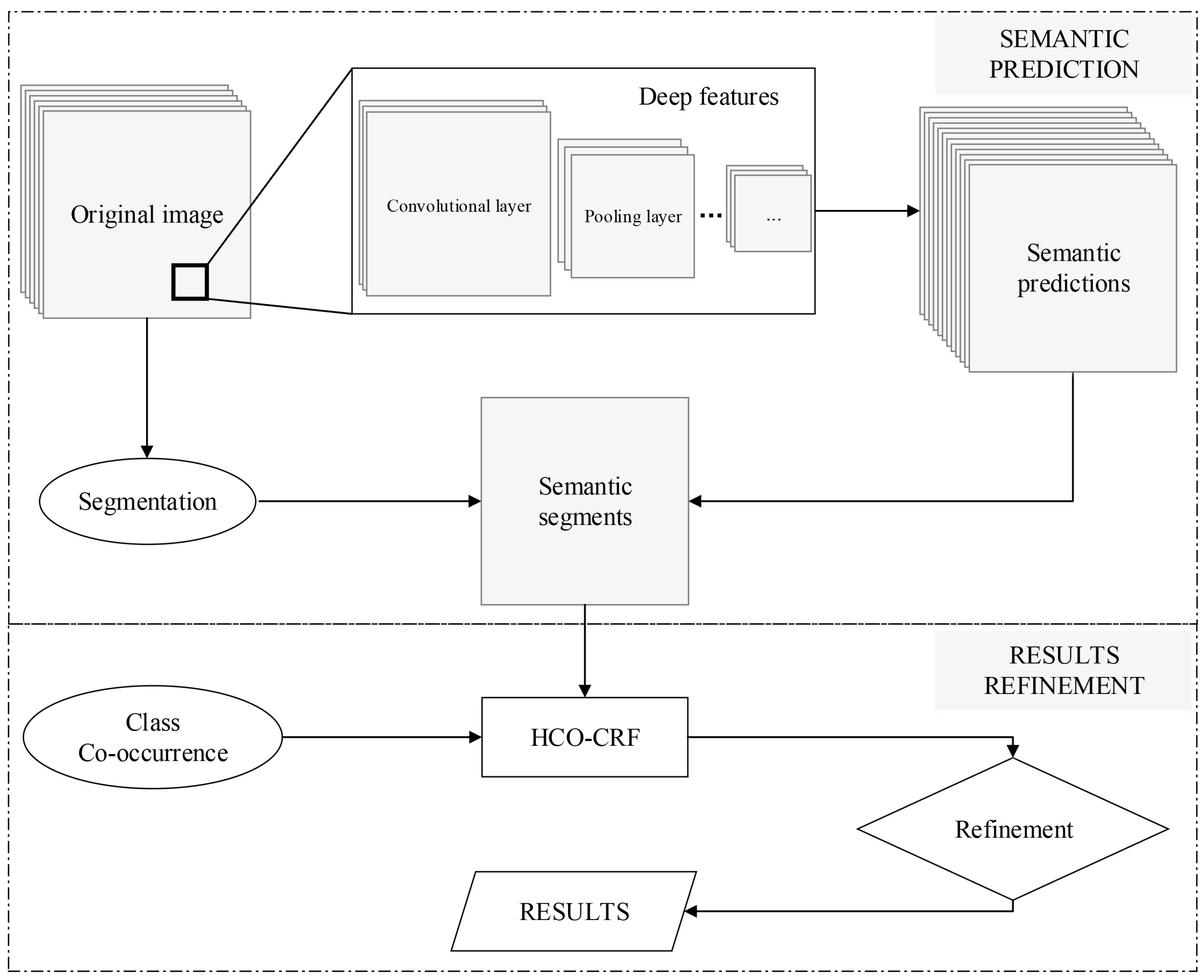
In this section, we build a higher-order co-occurrence graph model with the help of a semantic segmentation strategy. The proposed method is mainly constituted by two processing stages, i.e., semantic prediction and results refinement, as shown in Figure 1. For the process of semantic prediction, a CNN with five layers was trained using the reference dataset. After the training stage, the well-trained CNN can be directly applied to predict semantic labels for each pixel of the original image. Meanwhile, the predicted results of pixels were integrated with segments generated by the image segmentation algorithm. The integration of segments and semantic prediction results will produce semantic segments which are initial probabilistic per-class labeling predictions for each geographical object. Then, for the results refinement, the higher-order graph model can be constructed on top of semantic segments. It effectively formulates contextual information that could be further utilized to correct false predictions with the help of class co-occurrences and dependencies.

3.1. Semantic Segmentation with CNN

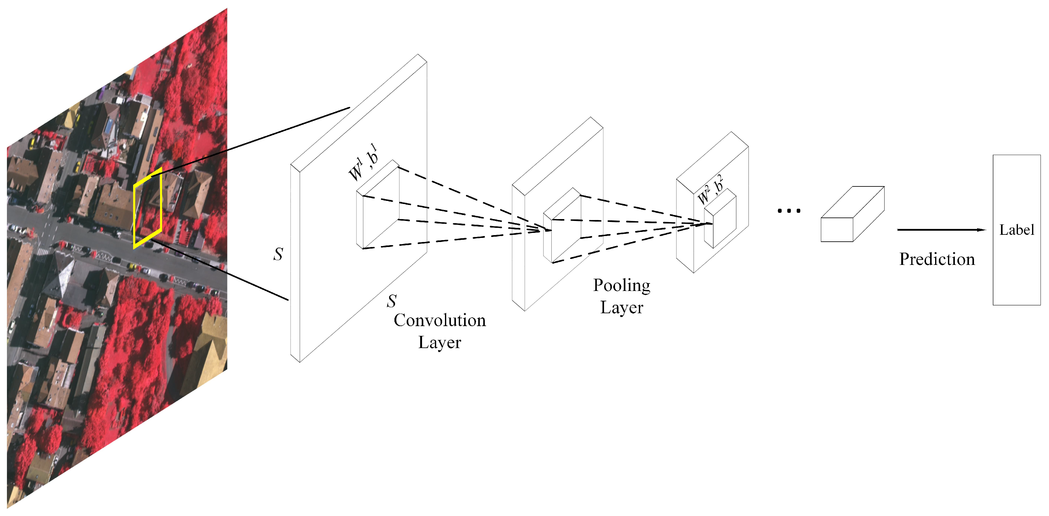
In this study, in order to obtain deep and robust feature representations of high-resolution imagery, we proposed an L-layer convolutional neural network, as shown in Figure 2. Given an image I and its corresponding reference map R. Since the CNN only feeds using square image patches, we split the input image I using a fixed square window with the sizes of $\mathcal{S}\ast \mathcal{S}$ with having targeted pixel in the center. For a pixel i in the original image, the extracted image patch can be represented as $P_i$ and its label $l_i$ obtained from the reference map. Before CNN can be used to extract deep features, two types of trainable parameters should be determined, i.e., convolutional filters $\mathbf{W}$ and the biases $\mathbf{b}$. Before training, we initialized all parameters with a zero mean and variance [24]. For the process of the feed-forward pass, the output of $\ell -$th, $(\ell \in L)$ layer is given by

$$d^{\ell }=f\left({\mathbf{u}}^{\ell }\right),{\mathbf{u}}^{\ell }={\mathbf{W}}^{\ell }{d}^{\ell -1}+{\mathbf{b}}^{\ell }$$

(1)

here, ℓ denotes the current layer, the output activation function $f(·)$ is usually chosen to be the hyperbolic tangent function $f\left(x\right)=a\tanh \left(bx\right)$. For a multi-class problem with c classes and N training samples. The square-loss function used for CNN training can be written as

$$E^N=\frac{1}{2}\sum _{n=1}^N\sum _{k=1}^c{(t_k^n-y_k^n)}^2$$

(2)

where $y=d^L$ denotes the final output of the $L-$th layer CNN framework. In order to minimize the loss function, the back-propagation algorithm is applied.

Although the extracted deep features are able to describe complex image patterns, the interspersed geographic objects in high-resolution images are still unreachable, due to the large gap between pixels and geographical objects. Meanwhile, the object-based image classification method bridges the gap between image pixel and geographical objects for high-resolution imagery interpretation. Instead of using low-level image features, we segment the heterogeneous imagery with the extracted deep features, in order to obtain meaningful semantic segments (segments with semantic labels). For pixel $I_i$ in the original image, the extracted deep feature vector has the form of $d_i=[d_i^1,d_i^2,\dots ,d_i^c]$. Then, we use the graph-based image segmentation algorithm to split the whole image $\mathbf{I}$ into N image segments using deeply extracted image features. Each image segment can be represented as $O_j,j\in \{1,2,\dots ,N\}$, and, there are M pixels $I_i,i\in \{1,2,\dots ,M\}$ inside each image object $O_j$. Thus, each image segment only has one significant semantic label.

$$\{O_1,O_2,\dots ,O_N\}\in \mathbf{I}$$

(3)

3.2. Contextual Refinement with HCO-CRF

Once the high-resolution image is delineated into meaningful regions, the complex geographical objects can be easily represented by semantic segments. As mentioned above, contextual information is vital for successful image labeling and understanding. Meanwhile, class co-occurrences as one of the most popular contextual feature descriptors in image classification has been widely used to exploit the contextual information, especially for high-resolution images [25]. Instead of using pixel-based CRF models, we constructed the segment-based CRF model with semantic segments. In the segment-based CRF model, each node represents a semantic segment. The weights of the neighboring matrix for segment-based CRF are determined by shared boundaries between adjacent semantic segments. In this way, the segment-based CRF model can effectively alleviate the phenomenon of local minima since it exploits contextual information at larger scales. At the same time, the usage of co-occurrence correction in the post-processing stage increased the label consistency between semantic segments also avoid the local minimum.

Instead of pixel-based CRF, we use semantic segments as the building blocks of the segment-based CRF. Therefore, the unary term potential for a semantic segment $O_j$ which contains K image pixels can be formulated as

$${\varphi }_j(y_j;O_j)={\varphi }_j(y_j;d_{j_1},d_{j_2},\dots ,d_{j_K})=-\sum _{k=1}^{K}H(d_{j_k},y_j)$$

(4)

where $y_j$ is the label of the semantic segment $O_j$, and $d_{j_k}$ represents the extracted deep features from the CNN framework. $H(·)$ is the output function with soft-max classifier which is given by $H(d_{j_k},y_j)=logp\left(y_j\right|d_{j_k}))$. In this unary potential, each semantic segment consists of a different number of image pixels. Therefore, the unary potentials of semantic segments are the sum of their pixels’ unary cost. Similarly, the pairwise potentials of Co-CRF have the form of

$${\varphi }_{ij}(O_i;O_j)=\frac{1}{1+\left|\right|O_{d_i}-O_{d_j}\left|\right|}$$

(5)

here, $O_{d_i}$ and $O_{d_j}$ are two averaged deep features which are located in semantic segments $O_i$ and $O_j$, respectively. Therefore, the entire cost function of the traditional CRF can be formulated as

$$E(y;d)=-\sum _{i\in O_i}\sum _{k=1}^{n_i}H(y_i,d_{i_k})+\sum _{O_i,O_j}\frac{1}{1+\left|\right|O_{d_i}-O_{d_j}\left|\right|}$$

(6)

However, the contextual information which is a key condition for accurate image labeling, which still remains to be exploited. In order to improve the accuracy of image classification, the co-occurrence of considering neighboring regions is naturally integrated with pairwise potentials. At the same time, class co-occurrence as prior information could easily be acquired from reference maps. To calculate the class co-occurrence, instead of using image segments, we count the adjacent pixels and their labels bilaterally through training images. As a result, the neighboring co-occurrence matrix of $c\times c$ can be built on sample statistics. Let $N_{m,l},(k\ne l)$ denote the number of co-existing labels of k and l, where both $m,l\in \{1,2,\dots ,c\}$. Thus, the frequency of co-occurrence labels $(m,l)$ is $c_{m,l}=\frac{N_{m,l}}{N_{all}}$, where $N_{all}$ represents the number of all possible co-occurrence label pairs. Based on the co-occurrence matrix, we can rewrite CRF pairwise potentials form

$$E(y;d)=-\sum _{i\in O_i}\sum _{k=1}^{n_i}H(y_i,d_{i_k})+\sum _{O_i,O_j}\frac{c_{m,l}}{1+\left|\right|O_{d_i}-O_{d_j}\left|\right|}$$

(7)

Although the revised CRF algorithm incorporates pairwise potentials and the label co-occurrence cost that fit the prior knowledge, the contextual information that lies in larger scale ranges still remain unexploited. In order to formulate the class-dependencies at larger scales, it is important to introduce the higher-order co-occurrence CRF (HCO-CRF) model, as shown in Figure 3. Different from the traditional CRF, the HCO-CRF captures class co-occurrences on top of semantic segments and avoids the ambiguities by incorporating higher-level context. An additional regulation term that describes higher order cliques has been added to the co-occurrence CRF model. Therefore, the formulation of HCO-CRF can be written as

$$E(y;d)=-\sum _{i\in O_i}\sum _{k=1}^{n_i}H(y_i,d_{i_k})+\sum _{O_i,O_j}\frac{c_{m,l}}{1+\left|\right|O_{d_i}-O_{d_j}\left|\right|}+\sum _{O_i\in T}\varphi \left(O_i\right)$$

(8)

Here, T represents the set of semantic segments obtained from the process of semantic segmentation, and, the term $\varphi \left(O_i\right)$ denotes higher order potentials which are defined over the segments. In order to formulate higher order terms, the $P^N$ Potts potential has been widely applied. It formulates as

$$\varphi \left(O_i\right)=\left\{\begin{array}{ll}\frac{n_i\left(O_i\right){\lambda }_{max}}{Q},& if{n}_i\left(O_i\right)<Q\\ {\lambda }_{max},& otherwise\end{array}\right.$$

(9)

The $n_i\left(O_i\right)$ is the number of pixels inside of the segment $O_i$ that take different labels from the dominant label. Meanwhile, the ${\lambda }_{max}={\theta }_i|O_i|,|O_i|$ counts the number of pixels inside of the segment. Q is the truncation parameter that controls the heterogeneity inside of the segment. In our experiments, the parameters Q and $\theta$ can be determined by applying cross-validation. Finally, the $\alpha -$expansion algorithm is applied to minimize the cost function in an iterative way.

4. Experiments and Analysis

4.1. Experimental Datasets

In order to illustrate the effectiveness of the HCO-CRF algorithm, we choose the Vaihingen dataset as the test dataset. The Vaihingen dataset was provided by the German Society for Photogrammetry, Remote Sensing, and Geoinformation (DGPF). It includes 38 image patches with a spatial resolution of 0.09 m for each pixel. In this experiment, we chose the scene 3 (Vaihingen 3) as the standard dataset for the rest of our work, it contains 1504 × 1003 pixels and five different types of land-cover. This dataset was acquired over the city of Vaihingen and is mainly composed of complex urban constructions, which made it challenging in terms of high-resolution image classification. Since the resolution of this dataset is relatively high, it reveals much more complex patterns at finer scales, such as car windows and road marks. Meanwhile, the computational costs of classifying such high-resolution images are prohibitive for real applications. Therefore, in this study, we subsampled the large image dataset to accelerate the classification process. Also, the Vaihingen images are colour-infrared aerial photos, which contain three bands that are infrared (IR), red (R) and green (G). The selected urban scene mainly composed of small residential houses (two or three floors), roads, some sparse trees, and vegetated areas, as shown in Figure 4a,b.

To further demonstrate the adaptiveness of the proposed method, a Worldview-2 dataset is also included in our experiments. The worldview-2 dataset has a spatial resolution of 1.8 m for each pixel, so coarser than the 0.09 m of the Vaihingen dataset. It was captured over the Beijing area by the Worldview-2 satellite in 2008. It contains 8 bands ranging from 0.45 to 1.04 $\mathsf{\mu }$m. The sizes of this dataset are $500\times 500$ pixels and there are six classes inside of the scene: bare soil, building, road, shadow, river, and vegetation.

4.2. Parameter Settings

In this experiment, we explored non-overlap image samples which were used for training and testing. The overlap threshold between two adjacent samples was set to 80%. The Vaihingen dataset has a spatial resolution of 0.09m, so there are thousands of pixels within an individual roof. Therefore the intra-class variation is much more challenging for the Vaihingen data in comparison to the Beijing dataset. Consequently, many more training samples are needed for the CNN to capture the complex spatial patterns in the Vaihingen dataset, that are needed for the Beijing data. Moreover, all training samples were randomly selected, and detailed information about training samples (TR) and validation samples (VA) is reported in

Table 1. Vaihingen scene: classes, training and validation samples.

Class	TR	VA
Building	5167	2582
Trees	1997	996
Grass	2772	1384
Cars	150	73
Road	6231	3113
Total	16,317	8148

and

Table 2. Beijing scene: classes, training and validation samples.

Class	TR	VA
Bare soil	150	741
Building	150	1803
Road	150	2065
Shadow	150	608
River	150	860
Vegetation	150	1021
Total	900	5898

.

Before high-resolution image classification, we first set up a well studied five-layer CNN framework [26] to extract deep features for remote sensing images. More specific, the CNN feeds with $28\times 28$ image patches with labeled pixels in the center. For the first convolutional layer, the input is converted to $24\times 24\times 20$ with 20 filters of $5\times 5$, before being subsampled with a $2\times 2$ max-pool layer to obtain a $12\times 12\times 20$ output. Then, the second convolutional layer includes 50 filters with the size of $5\times 5$ to generate an $8\times 8\times 20$ output, which is then subsampled to $4\times 4\times 20$ with the max-pool operator. Finally, a fully connected dense layer with 256 hidden units is used before resolving our different labels in a softmax output layer. The learning rate was set to 0.0001.

The co-occurrence matrix for the selected scene was acquired previously using sample statistics over the reference map. For the Vaihingen dataset, we utilized the entire reference map to calculate co-occurrences between different targets. The co-occurrence matrix of Vaihingen dataset is illustrated in

Table 3. Co-occurrence matrix of Vaihingen dataset. Building: BD, TE: Trees, GA: Grass, CA: Cars, RD: Road.

	BD	TE	GA	CA	RD
BD	0.6480	0.0691	0.1330	0.0167	0.1025
TE	0.0691	0.5830	0.1823	0.0583	0.1543
GA	0.1330	0.1823	0.5477	0.0500	0.0901
CA	0.0167	0.0583	0.0500	0.2333	0.0139
RD	0.1025	0.1543	0.0901	0.0139	0.6392

. This shows that the co-occurrence matrix is a symmetric matrix with the largest value in the diagonal direction. From this matrix, we concluded that adjacent pixels or objects are more likely to be the same class rather than different classes, and that around an objects’ edges a mixture of classes is observed. Therefore, based on the co-occurrence matrix, we can further correct classification errors based on knowledge of expected patterns of class co-occurrence. For the Beijing dataset, it is difficult to statistically analyze the co-occurrence matrix since the reference labels are scarce. For the purpose of obtaining class dependency information, we’ve performed CNN-based classification using training samples. Then, the co-occurrence matrix

Table 4. Co-occurrence matrix of Beijing dataset. Bare soil: BS, Buildings: BD, Road: RD, Shadow: SD, River: RV, Vegetation: VG.

	BS	BD	RD	SD	RV	VG
BS	0.4600	0.0521	0.0466	0.1503	0.2344	0.0410
BD	0.0521	0.6681	0.1400	0.1937	0.0156	0.0271
RD	0.0466	0.1400	0.7317	0.1373	0.1094	0.1660
SD	0.1503	0.1937	0.1373	0.3910	0.0313	0.0219
RV	0.2344	0.0156	0.1094	0.0313	0.2500	0.0024
VG	0.0410	0.0271	0.1660	0.0219	0.0024	0.7416

can be derived from the classification map. Although the classification results may not be as accurate as the hand-crafted reference map, it generally indicates the observed patterns of class dependencies in terms of adjacent rules. Therefore, we referred the statistical results as the co-occurrence matrix which could be applied to improve the classification results.

The parameter settings of HCO-CRF are determined by using a cross-validation procedure. As illustrated in the cost function of the higher-order CRF model, both the initial classification results and co-occurrence matrix $c_{m,l}$ can be automatically deduced from prior information. For the higher-order term, it is necessary to choose the optimal parameters in order to achieve good classification results. To minimize the HCO-CRF cost function, we performed the cross-validation procedure by tuning Q and $\theta$, respectively. To be more specific, we set the range of Q from 0.1 to 0.4 with the step of 0.1 and set the $\theta$ from 0.5 to 1.2 with the same step, as shown in

Table 5. Setting parameters for the higher-order term.

	θ	0.5	0.6	0.7	0.8	0.9	1.0	1.1	1.2
Q
0.1		88.72	88.69	88.63	88.51	87.92	88.01	87.37	84.82
0.2		86.23	87.31	88.85	89.05	89.12	89.08	89.16	88.91
0.3		86.48	86.18	88.01	88.47	89.13	89.10	89.15	89.03
0.4		85.94	86.79	87.63	88.26	88.87	89.01	88.79	88.45

. After the process of cross-validation, we set $Q=0.3$ and $\theta =1.1$ for our experiments.

4.3. Experimental Results

4.3.1. Vaihingen Dataset

After the CNN training, the deep features of the Vaihingen dataset can be easily acquired. We then split the Vaihingen scene into homogeneous regions based on robust deep features. Since we only utilized image segments to keep image edge information, the segmentation scale was set to 50. In order to illustrate the effectiveness of the proposed method, we compared it with other benchmark methods that are used for image classification. For instance, the Extended Morphological Profiles (EMP) with areas {50, 500} and standard deviation ranges from 2.5% to 20%. Meanwhile, we employed the pixel-based CNN (PCNN) and object-based CNN (OCNN) methods to illustrate improvements compared to the standard CNN method. Also, we included the fully connected CRF (i.e., Dense CRF) method to further improve the classification results of the OCNN. The classification maps with different methods are shown in Figure 5. Meanwhile, we selected the training samples according to the class ratios for available samples. In order to demonstrate the robustness of our method, we only chose 10% available samples (satisfies the overlap condition) for CNN training and another 5% for validation, and the detailed information about classification accuracies is listed in the

Table 6. Classification results of Vaihingen dataset with different strategies (in percentage). OA: Overall Accuracy.

Class	EMP	PCNN	OCNN	Dense CRF	HCO-CRF
Building	75.99	88.83	90.82	91.73	94.28
Trees	74.36	73.08	73.50	72.84	91.13
Grass	61.41	66.88	67.55	67.91	71.79
Cars	3.99	29.41	29.87	32.57	40.21
Roads	85.13	88.54	89.92	90.16	91.09
OA	75.33	80.30	82.03	83.53	86.52
Kappa	0.66	0.73	0.75	0.79	0.81

.

Due to the variable nature of high-resolution image datasets, it is difficult to accurately classify complex urban scenes into semantic maps. As shown in Figure 5, the SVM classification method which only utilized spectral information, it has the worst performance in terms of interpretation accuracies. The reason behind this phenomenon is that different land-cover objects are highly mixed together in the spectral feature space. To improve the performance of high-resolution image classification, the EMP-based method was proposed. It overcomes spectral variation and generates spatial descriptors using various spatial filters under different configurations. In general, the EMP-based methods both rely on low-level image features which lead to a failure in terms of high-resolution image classification. The CNN can automatically learn complex image patterns that could be used for efficient classification. Therefore, we introduced the well-known PCNN for comparison. In general, the PCNN method is much better than the traditional method in terms of classifying complex buildings and cars. Generally, the building classification accuracies increased from 75.99% to 88.83%. However, the accurate mapping rate still ranges from 3.99% to 29.41% for the car class. The cause of this phenomenon should be the unbalanced training sample settings where only 150 car samples compare to other classes with a large number of training samples. But, it is impossible to keep the balance for different types of training samples as the car are quite small compared to other geographical objects.

In general, the PCNN method can effectively increase the classification accuracy at the pixel level. However, many geographical objects in images that are poorly characterised are crucial for understanding the image and accurate mapping. Thus, we introduced the Dense CRF method in order to classify high-resolution images more efficiently. From the classification results, we can conclude that the classification accuracy of building and road have significantly increased at the object level (OCNN). However, the Dense CRF method only enforces smoothness over adjacent objects and regardless the co-occurrences between them. Finally, we compared the previous classification results with the HCO-CRF method. With the introduction of co-occurrence information between different objects, the initial classification results can be further refined.

4.3.2. Beijing Dataset

In order to keep a balanced training samples, we selected 150 samples for each class for the CNN training. After the training process, we applied the well-trained CNN to extract deep features and obtain the initial classification results. Also, the segmentation scale was set to 30, in order to get accurate information about shapes and edges of geographical objects. With the integration of image segments and the CNN-based classification results, the classification accuracy can be further improved. Moreover, the PCNN, OCNN and Dense CRF methods were included to demonstrate the effectiveness of the proposed method. The classification results are illustrated in Figure 6. The detailed information about classification accuracies is shown in

Table 7. Classification results of Beijing dataset with different strategies (in percentage). OA: Overall Accuracy.

Class	EMP	PCNN	OCNN	Dense CRF	HCO-CRF
Bare soil	79.76	84.71	90.32	97.38	99.06
Buildings	70.93	89.91	95.06	97.26	98.29
Roads	95.09	95.92	97.65	98.07	99.19
Shadows	98.91	95.78	96.67	84.32	85.42
Rivers	100	78.27	80.63	83.28	88.91
Vegetation	92.64	77.68	75.30	89.42	91.88
OA	86.99	89.03	92.61	95.61	97.42
Kappa	0.81	0.85	0.89	0.91	0.94

.

Comapred to the Vaihingen dataset, the Beijing dataset has a coarser spatial resolution but with significant richer spectral information. Moreover, the geographical objects such as buildings are much blurrier than what appeared in the Vaihingen scene. At first, we applied the EMP algorithm to classify the Beijing dataset by using spectral information. It is efficient to detect natural geographical objects with significant spectral differences, such as shadow, water, and vegetation. With the help of EMP features, it is difficult to capture the complex buildings with higher accuracies. As for the CNN framework, the classification accuracy of buildings has increased from 79.76% to 84.71%. However, due to the limited number of deep features, the rivers and vegetation suffer a significant drop, in terms of classification accuracies. This is probably because their deep spectral features are limited and their spectral properties are highly distinctive. At last, the HCO-CRF further refined the classification results by introducing the higher-order co-occurrence term. For instance, the classification accuracies of road and building can be as high as 99.19% and 98.29%. Therefore, it further demonstrated that the proposed method is capable to accurately classify complex urban scenes.

5. Discussion

5.1. Semantic Segments Extraction

In order to extract semantic information from the high-resolution remote sensing imagery, it is important to design accurate classification procedures to perform image labeling. At the same time, image features representatively describe the characteristics of image targets. Based on the effective descriptions of the image pattern, image targets with distinctive characters can be effectively discriminated. However, as the spatial resolution gets finer, traditional feature representations may not be distinctive enough to differentiate image targets with similar patterns, e.g., building roofs and road surface with similar materials. In this regard, we introduced a deep learning strategy to extract more robust and representative features from higher conceptual levels. To be specific, the convolutional neural network (CNN) was applied to automatically generate hierarchical features by feeding square-sized image patches. For the conventional CNN, it usually consists of convolutional layers and pooling layers. For the convolutional layer, numbers of image filters with learnable parameters are stacked together to perform image filtering. Given the outputs of the convolutional layer, the pooling layer directly shrinks the sizes of the output feature maps and further strengthen the robustness of the extracted features. Compare to the traditional image feature representations, the extracted deep features are much more effective in terms of exploiting the small differences. Therefore, we applied the CNN model to perform dense labeling of high-resolution imagery. Still, the classification results of the CNN model suffers from the spatial information loss and “salt–pepper” noise. Moreover, the classification results in mere pixel-level labeling which has no access to geographical entities. To extract semantic information from high-resolution imagery, it is necessary to map the targets at the object level. In this study, instead of using CNN to directly predict the semantic information of each pixel, we integrated the results of dense labeling and image segments. In this way, spatial information about geographical targets can be kept intact. For each image segment, the simple majority vote is applied to determine the semantic label of the segment. As a result, the high-resolution image is delineated into semantically uniform regions that each part represents a geographical target. Based on the results of semantic segmentation, rich semantic information of the high-resolution image can be automatically extracted.

5.2. Higher-Order Contextual Formulation

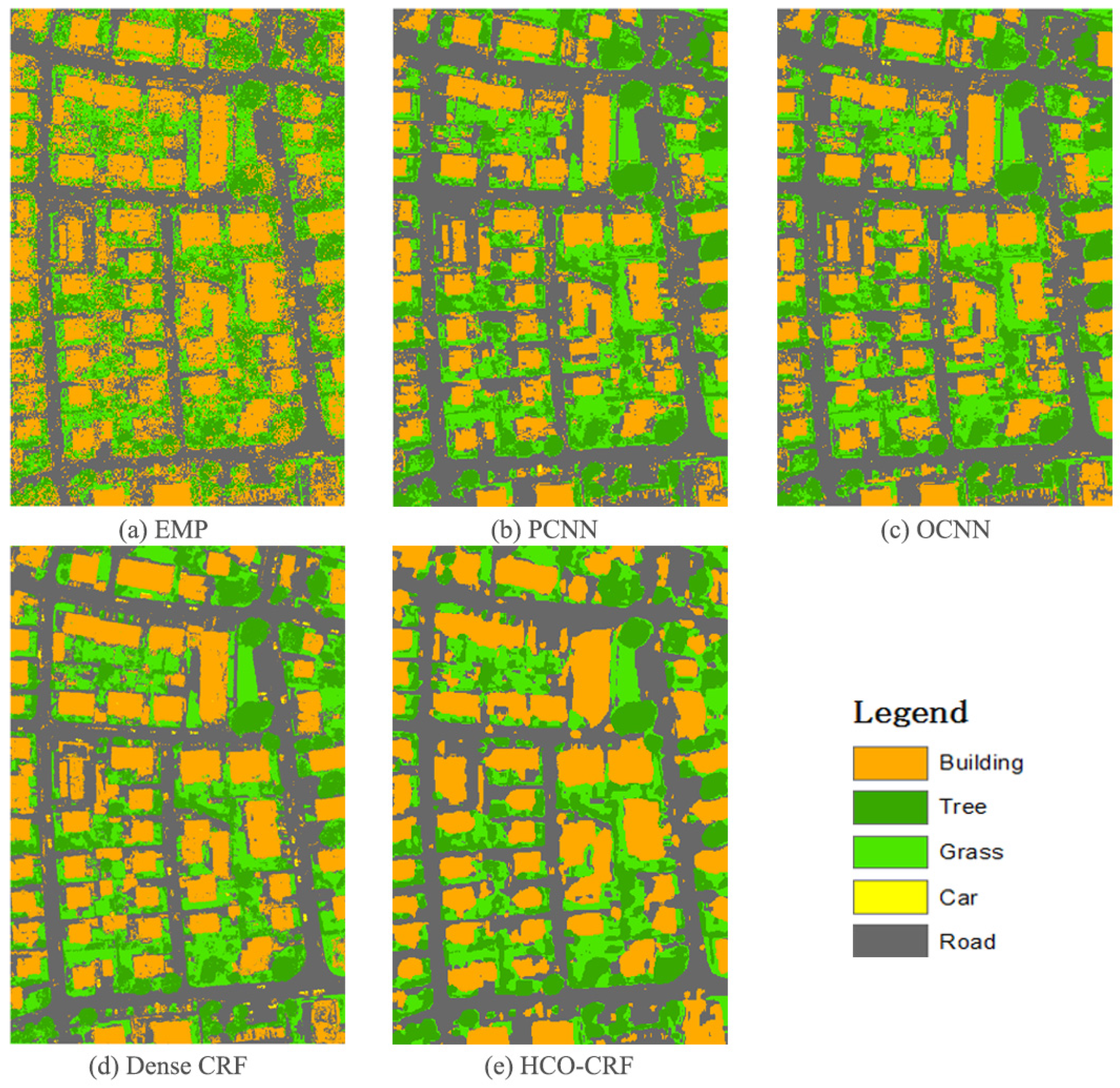
Given the results of semantic segmentation, it is easy to access the semantic contents of the high-resolution images. Although, the classification accuracy of the CNN-based method is usually higher than the conventional pixel- or object-based methods, still, small errors are frequently observed from CNN-based classification results. For instance, road surfaces may share similar texture or spatial patterns with building roofs which make classifiers difficult to distinguish them from each other. The reason for this phenomenon is that the CNN model is only fed with a square window that neglected the global context. To better grasp the contextual information, post-processing models such as CRF are one way to formulate the image context. CRF mainly exploits the prior knowledge such as the fact that nearby pixels (in the spatial or feature domain) likely share the same semantic label. The standard CRF model usually consists of unary and pairwise terms in a fashion of 4- or 8-connected neighborhood. With the help of the CRF model, the classification results of the high-resolution image can be further improved. For one thing, the pixel-based classification refinement often suffers from “salt-pepper” noise, therefore, it is necessary to build a CRF model on top of image segments. Image segments can capture richer contextual information than a single pixel. Also, the computational costs can be greatly reduced if one considers pairwise interactions between image segments rather than pixels. For another, the conventional CRF model only formulates the local pairwise potentials that capture interactions between pairs of image pixels or segments. Thus, the conventional CRF model works like a smoother at the local range and neglect the long-range context of the high-resolution image. To capture more contextual information at longer ranges, we formulated the CRF model with a higher order potential. It directly captures the interactions over cliques larger than just two nodes. Therefore, it provides a better way to model the co-occurrences between geographical objects and further improving classification results.

6. Conclusions

In this paper, we proposed a graph-based model to classify high-resolution images by considering higher-order co-occurrence information. To be more specific, instead of using low-level image features, we investigated the CNN-based deep features for image semantic segmentation. Then, based on the extracted semantic segments, we utilized the graph-based CRF model to capture the contextual information for better classification results. At last, we further improved the CRF-based classification results by considering higher-order co-occurrences between different geographical objects. In order to illustrate the effectiveness of the proposed method, we compared the HCO-CRF method with other commonly used high-resolution image classification methods. The classification results indicate that the HCO-CRF method can effectively refine classification based on the co-occurrence of different classes. However, the parameter of the co-occurrence matrix should be defined in prior to the loss function minimization done during the training process of the HCO-CRF training. In future research, the quantitative measurements over geographical objects, such as co-occurrences and spatial relationships should be thoroughly studied.

References

1. Huang, X.; Lu, Q.; Zhang, L. A multi-index learning approach for classification of high-resolution remotely sensed images over urban areas. ISPRS J. Photogramm. Remote Sens. 2014, 90, 36–48. [Google Scholar] [CrossRef]
2. Liu, Q.; Hang, R.; Song, H.; Li, Z. Learning Multiscale Deep Features for High-Resolution Satellite Image Scene Classification. IEEE Trans. Geosci. Remote Sens. 2017, 56, 117–126. [Google Scholar] [CrossRef]
3. Hang, R.; Liu, Q.; Song, H.; Sun, Y. Matrix-based discriminant subspace ensemble for hyperspectral image spatial–spectral feature fusion. IEEE Trans. Geosci. Remote Sens. 2016, 54, 783–794. [Google Scholar] [CrossRef]
4. Soh, L.K.; Tsatsoulis, C. Texture analysis of SAR sea ice imagery using gray level co-occurrence matrices. IEEE Trans. Geosci. Remote Sens. 1999, 37, 780–795. [Google Scholar] [CrossRef] [Green Version]
5. Dalla Mura, M.; Benediktsson, J.A.; Waske, B.; Bruzzone, L. Morphological attribute profiles for the analysis of very high resolution images. IEEE Trans. Geosci. Remote Sens. 2010, 48, 3747–3762. [Google Scholar] [CrossRef]
6. Dalla Mura, M.; Villa, A.; Benediktsson, J.A.; Chanussot, J.; Bruzzone, L. Classification of hyperspectral images by using extended morphological attribute profiles and independent component analysis. IEEE Geosci. Remote Sens. Lett. 2011, 8, 542–546. [Google Scholar] [CrossRef]
7. Zhao, W.; Du, S. Learning multiscale and deep representations for classifying remotely sensed imagery. ISPRS J. Photogramm. Remote Sens. 2016, 113, 155–165. [Google Scholar] [CrossRef]
8. Zhao, W.; Du, S. Scene classification using multi-scale deeply described visual words. Int. J. Remote Sens. 2016, 37, 4119–4131. [Google Scholar] [CrossRef]
9. Blaschke, T. Object based image analysis for remote sensing. ISPRS J. Photogramm. Remote Sens. 2010, 65, 2–16. [Google Scholar] [CrossRef]
10. Blaschke, T.; Hay, G.J.; Kelly, M.; Lang, S.; Hofmann, P.; Addink, E.; Feitosa, R.Q.; van der Meer, F.; van der Werff, H.; van Coillie, F.; et al. Geographic object-based image analysis–towards a new paradigm. ISPRS J. Photogramm. Remote Sens. 2014, 87, 180–191. [Google Scholar] [CrossRef] [PubMed]
11. Ghamisi, P.; Benediktsson, J.A.; Ulfarsson, M.O. Spectral–spatial classification of hyperspectral images based on hidden Markov random fields. IEEE Trans. Geosci. Remote Sens. 2014, 52, 2565–2574. [Google Scholar] [CrossRef]
12. Kasetkasem, T.; Arora, M.K.; Varshney, P.K. Super-resolution land cover mapping using a Markov random field based approach. Remote Sens. Environ. 2005, 96, 302–314. [Google Scholar] [CrossRef]
13. He, X.; Zemel, R.S.; Carreira-Perpiñán, M.Á. Multiscale conditional random fields for image labeling. In Proceedings of the 2004 IEEE Computer Society Conference on Computer Vision and Pattern Recognition, Washington, DC, USA, 17 June–2 July 2004; IEEE: Piscataway, NJ, USA, 2004; Volume 2. [Google Scholar]
14. Zhang, G.; Jia, X. Simplified conditional random fields with class boundary constraint for spectral-spatial based remote sensing image classification. IEEE Geosci. Remote Sens. Lett. 2012, 9, 856–860. [Google Scholar] [CrossRef]
15. Wegner, J.D.; Hansch, R.; Thiele, A.; Soergel, U. Building detection from one orthophoto and high-resolution InSAR data using conditional random fields. IEEE J. Select. Top. Appl. Earth Obs. Remote Sens. 2011, 4, 83–91. [Google Scholar] [CrossRef]
16. Zhong, Y.; Zhao, J.; Zhang, L. A hybrid object-oriented conditional random field classification framework for high spatial resolution remote sensing imagery. IEEE Trans. Geosci. Remote Sens. 2014, 52, 7023–7037. [Google Scholar] [CrossRef]
17. Zhao, W.; Du, S.; Wang, Q.; Emery, W.J. Contextually guided very-high-resolution imagery classification with semantic segments. ISPRS J. Photogramm. Remote Sens. 2017, 132, 48–60. [Google Scholar] [CrossRef]
18. Romero, A.; Gatta, C.; Camps-Valls, G. Unsupervised deep feature extraction for remote sensing image classification. IEEE Trans. Geosci. Remote Sens. 2016, 54, 1349–1362. [Google Scholar] [CrossRef]
19. Maggiori, E.; Tarabalka, Y.; Charpiat, G.; Alliez, P. Convolutional Neural Networks for Large-Scale Remote-Sensing Image Classification. IEEE Trans. Geosci. Remote Sens. 2017, 55, 645–657. [Google Scholar] [CrossRef]
20. Fu, G.; Liu, C.; Zhou, R.; Sun, T.; Zhang, Q. Classification for high resolution remote sensing imagery using a fully convolutional network. Remote Sens. 2017, 9, 498. [Google Scholar] [CrossRef]
21. Long, J.; Shelhamer, E.; Darrell, T. Fully convolutional networks for semantic segmentation. In Proceedings of the IEEE Computer Society Conference on Computer Vision and Pattern Recognition, Boston, MA, USA, 7–12 June 2015; pp. 3431–3440. [Google Scholar]
22. Kohli, P.; Torr, P.H.; Ladicky, L. Robust higher order potentials for enforcing label consistency. Int. J. Comput. Vis. 2009, 82, 302–324. [Google Scholar] [CrossRef]
23. Li, E.; Femiani, J.; Xu, S.; Zhang, X.; Wonka, P. Robust rooftop extraction from visible band images using higher order CRF. IEEE Trans. Geosci. Remote Sens. 2015, 53, 4483–4495. [Google Scholar] [CrossRef]
24. Glorot, X.; Bengio, Y. Understanding the difficulty of training deep feedforward neural networks. In Proceedings of the Thirteenth International Conference on Artificial Intelligence and Statistics, Chia Laguna Resort, Italy, 13–15 May 2010; Teh, Y.W., Titterington, M., Eds.; PMLR: Chia Laguna Resort, Italy, 2010; Volume 9, pp. 249–256. [Google Scholar]
25. Wang, L.; Huang, X.; Zheng, C.; Zhang, Y. A Markov random field integrating spectral dissimilarity and class co-occurrence dependency for remote sensing image classification optimization. ISPRS J. Photogramm. Remote Sens. 2017, 128, 223–239. [Google Scholar] [CrossRef]
26. Zhao, W.; Du, S. Spectral-Spatial Feature Extraction for Hyperspectral Image Classification: A Dimension Reduction and Deep Learning Approach. IEEE Trans. Geosci. Remote Sens. 2016, 54, 4544–4554. [Google Scholar] [CrossRef]
Figure 1. The flowchart of dense semantic labeling with higher-order co-occurrence graph model.
Remotesensing 10 01713 g001
Figure 2. Semantic prediction using Convolutional neural network.
Remotesensing 10 01713 g002
Figure 3. The illustration of HCO-CRF improvements. Based on the semantic segments, the initial classification result (left) can be further refined according to the co-occurrence matrix between classes (right).
Remotesensing 10 01713 g003
Figure 4. The illustration of experimental datasets and reference maps. (a,b) the Vaihingen dataset and its reference map, (c,d) the Beijing dataset and its reference map.
Remotesensing 10 01713 g004
Figure 5. Classification results on Vaihingen dataset with different strategies. (a) EMP-based classification; (b) pixel-based CNN classification; (c) the object-based CNN classification; (d) Dense CRF classification; (e) HCO-CRF classification result.
Remotesensing 10 01713 g005
Figure 6. Classification results on Beijing dataset with different strategies. (a) EMP-based classification; (b) pixel-based CNN classification; (c) the object-based CNN classification; (d) Dense CRF classification; (e) HCO-CRF classification result.
Remotesensing 10 01713 g006