Quantitative Assessment for Detection and Monitoring of Coastline Dynamics with Temporal RADARSAT Images

Abstract

This study aims to detect coastline changes using temporal synthetic aperture radar (SAR) images for the state of Kelantan, Malaysia. Two active images, namely, RADARSAT-1 captured in 2003 and RADARSAT-2 captured in 2014, were used to monitor such changes. We applied noise removal and edge detection filtering on RADARSAT images for preprocessing to remove salt and pepper distortion. Different segmentation analyses were also applied to the filtered images. Firstly, multiresolution segmentation, maximum spectral difference and chessboard segmentation were performed to separate land pixels from ocean ones. Next, the Taguchi method was used to optimise segmentation parameters. Subsequently, a support vector machine algorithm was applied on the optimised segments to classify shorelines with an accuracy of 98% for both temporal images. Results were validated using a thematic map from the Department of Survey and Mapping of Malaysia. The change detection showed an average difference in the shoreline of 12.5 m between 2003 and 2014. The methods developed in this study demonstrate the ability of active SAR sensors to map and detect shoreline changes, especially during low or high tides in tropical regions where passive sensor imagery is often masked by clouds.

1. Introduction

A coastline is defined as the boundary between land and water. It is an important and dynamic linear feature [1]. An accurate delineation of coastline can be used in coastal zone management and planning. A large percentage of the world’s population lives in coastal areas. Hence, these areas are under intense pressure from urban growth, industry and tourism [2]. A prerequisite for sustainable management of these environmentally sensitive areas is the availability of accurate and up-to-date information on the status and extent of change. For countries with large coastal areas, such as Malaysia, nautical products are useful sources of such information for military management and coastal zone management and planning [3].

An active radar product interacts differently with surface features from passive optical imagery [4], and it can also penetrate through clouds [5]. Radar imagery provides a large amount of useful information in terms of structure and shape rather than surface reflectance [6,7]. Therefore, they are valuable for many applications, such as disaster and natural resource management [3,8]. The information stored in multiple SAR polarisations may help reduce uncertainties in water delineation, which needs an optimised classification method other than single band image processing [9]. Any developed and soft coastlines, such as Peninsula lands, always have a continuous demand for an up-to-date, accurate and detailed map of the coastline [2]. Generally speaking, beaches have a dynamic change; thus, coastal zone monitoring is important for shoreline protection [10,11]. Field applications that rely on important tasks of shoreline change detection and monitoring include regional sediment yield, erosion–accretion, hazard zoning and setback planning [1,12].

Traditional field surveying methods by theodolites, GPS receivers, etc. are time-consuming and costly compared with remote sensing and geographical information system (GIS)-based methods [3,13]. Satellite imagery becomes one of the most useful sources of information for coastal monitoring [14]. However, in tropical regions, frequent cloud coverage is a major issue in optical satellite imagery and brings difficulty in delineation of land and ocean boundaries [15]. Identification of land and ocean boundaries is complicated using optical imagery due to cloud coverage [16]. The recent systematic tools of remote sensing and GIS are exceptionally important for coastal environmental studies and coastal zone management and planning [17]. However, monitoring coastline changes using synthetic aperture radar (SAR) images during high and low tides is challenging due to the mixed backscattering response resulting from the variation of wet and dry sands. This leads to misclassification problem when dealing with SAR image.

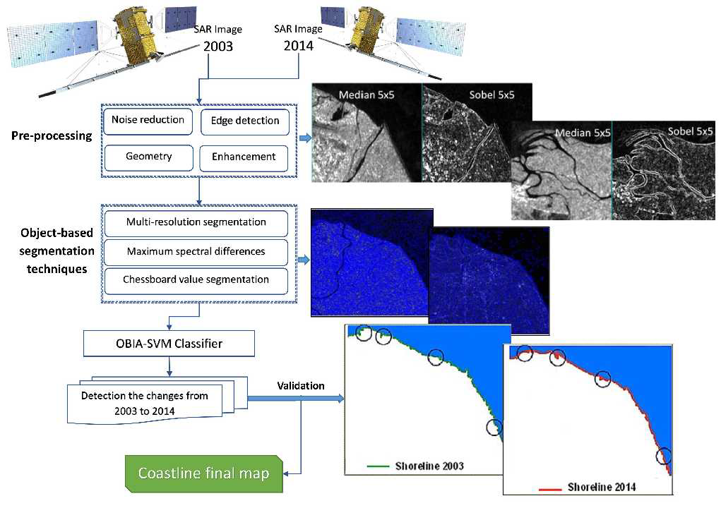
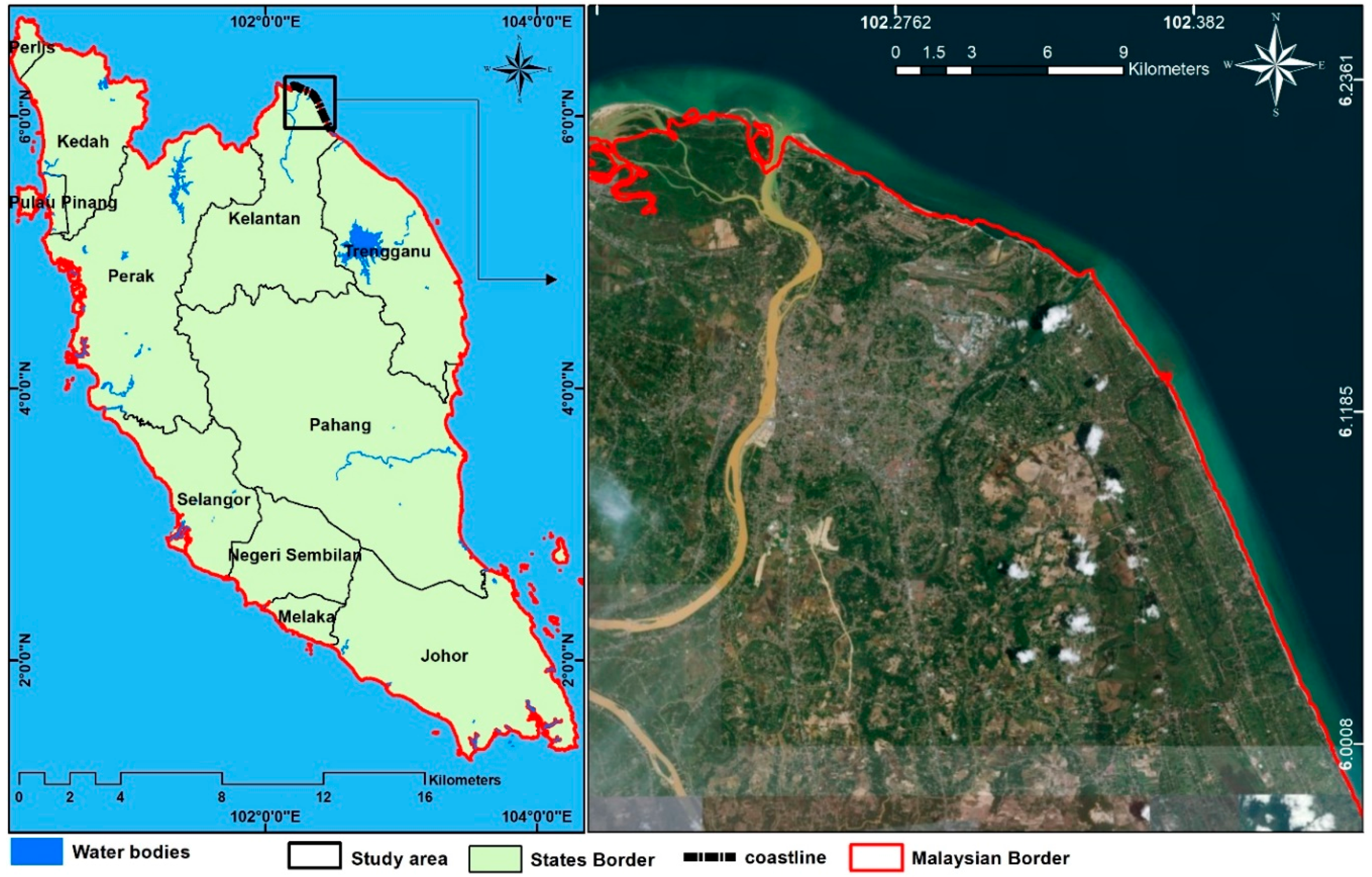
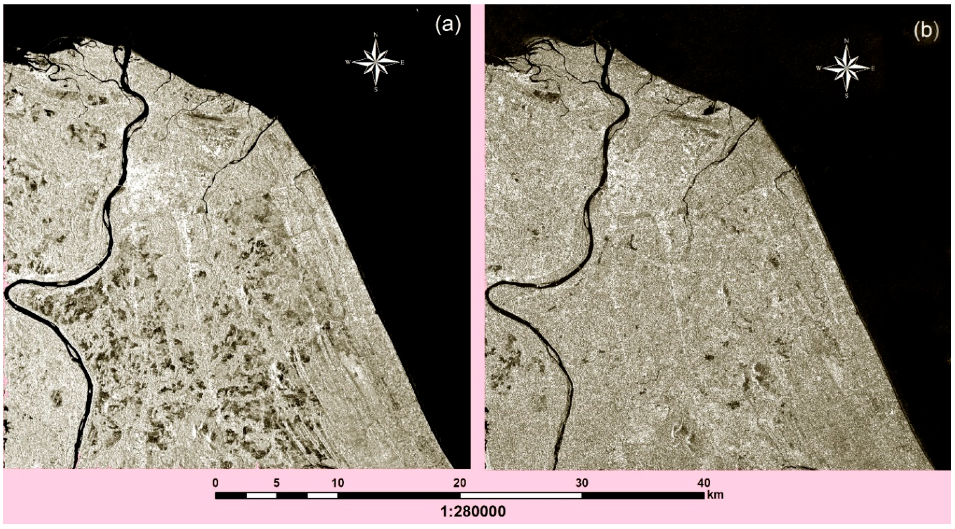
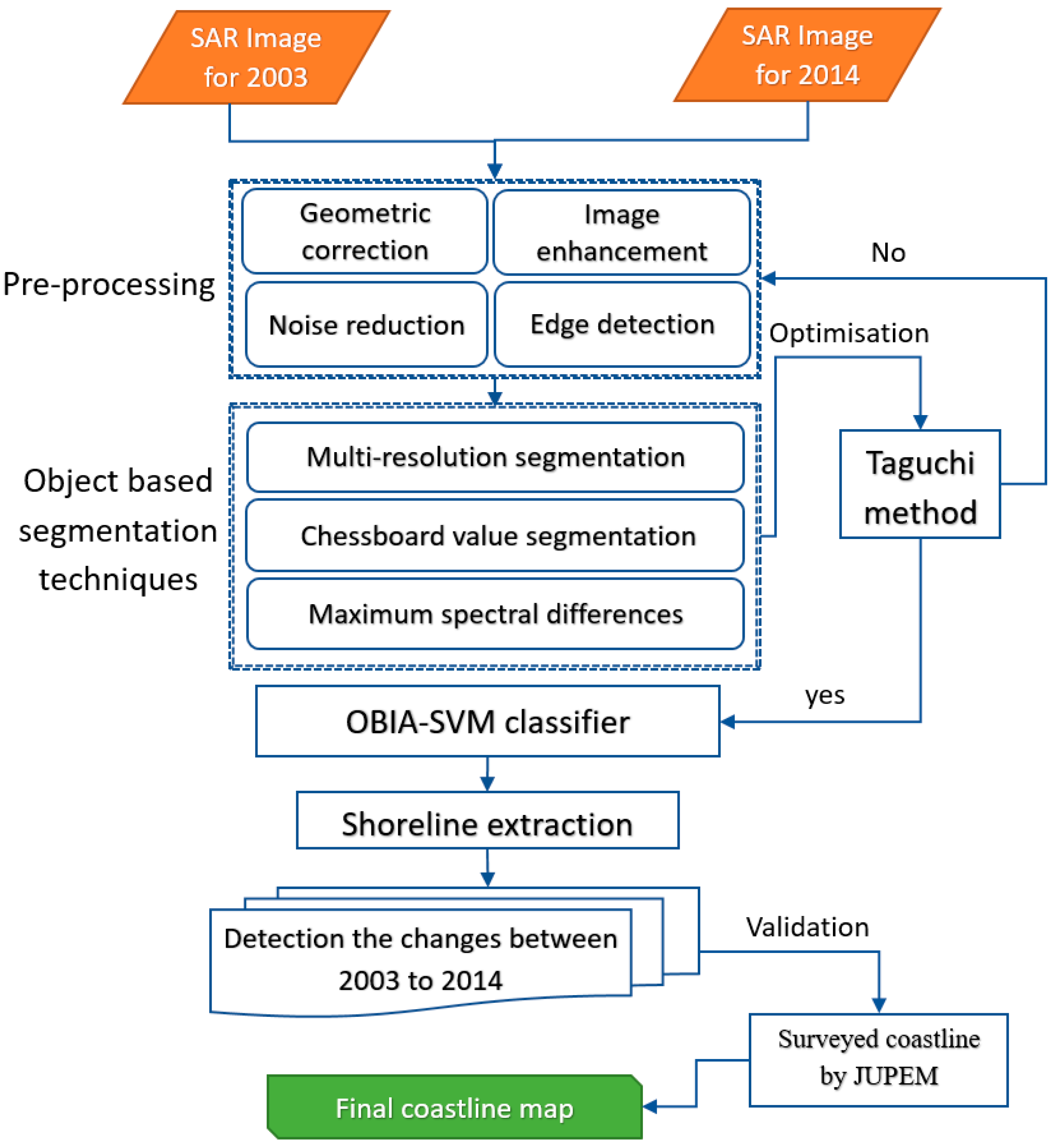
This research aims to identify the shoreline and assess the magnitude and direction of shoreline changes from 2003 to 2014 using SAR images. This study attempts to propose an optimised semiautomatic coastline detection method using temporal SAR images, which are subjected to notable environmental parameters, such as wind and large amounts of textural noise over the sea surface. We processed the SAR dataset to detect and monitor changes along the east coast of Kelantan, Malaysia, using two sets of RADARSAT images. The noises on SAR imagery were filtered out, and an adequate technique was then developed to discriminate lands from those noises. This process is critical in feature detection using SAR images, especially in coastal areas.

2. Materials and Methods

2.1. Study Area

Kelantan is in the north eastern part of Peninsular Malaysia. This area is bordered by Neratiwat from Thailand to the north, Terengganu to the southeast, Perak to the west and Pahang to the south. The study area is located between 6°00′30.67′′N and 102°44′16.05′′E and 6°25′11.00′′N and 102°16′18.00′′E (Figure 1). In the north of the Clayton Bay lies the South China Sea, which is the largest sea in Southeast Asia; a Sunda platform from the continental shelf exists with a depth of more than 100 m [18]. The annual temperature varies from 24 °C to 28 °C; the average humidity is approximately 80%. The cloud coverage over the sea ranges between 50% and 75%, and it has been observed to be steady over the years.

2.2. Datasets

We used two active SAR images, namely, RADARSAT-1 and RADARSAT-2, which operate in C-band frequency at a repeat cycle of 24 days. The images were acquired on 12 November 2003, and 12 November 2014, and cover the area of Tumpat-Kota Bharu District (Delta area) of Kelantan. The images were further cut on the basis of the area of interest (Figure 2).

Each RADARSAT data has different swath width, azimuth, range and incidence angle that was retrieved from single-look complex (SLC) data. To achieve the ground square pixels from RADARSAT images and to decrease the image speckle noise, multilooking procedure was implemented on both datasets by multiplying the multilook factors of sensor with the azimuth and range direction (

Table 1. Details of the satellite data and resolution.

Band Characteristics	RADARSAT-1	RADARSAT-2
Active antenna	C-Band	C-Band
Centre frequency	5.3 GHz	5.405 GHz
Bandwidth (maximum)	30 MHz	100 MHz
Polarization	HH	HV, HH, VH, VV
Polarization isolation	>20 dB	>25 dB
Incidence angle [degree]	41	41
Multilook (range × azimuth)	1 × 4	1 × 4
Pixel dimensions [m] (range × azimuth)	8 × 8 m	8 × 8 m

). Then, the resampled multilook intensity (MLI) images were obtained. The images with ground resolution of 8 m with HH polarisation were used for analysis. Subsequently, the preprocessing steps, including filtering and image enhancement, were applied on the MLI images that have similar spatial resolution characteristic to reduce the shoreline change detection uncertainties.

ENVI 5.3 software was used for image sharpening, edge and change detection. eCognition Developer 64 was used for segmentation and classification, and ArcGIS 10.4 was adopted for shoreline extraction and validation. Figure 3 shows the overall flowchart and methodology of this research.

The following sections describe the computational framework of preprocessing techniques on SAR images, segmentation experiments, optimisation process of segmentation parameters, classification of segmented images into water and land, shoreline border extraction for 2003 and 2014, detection of possible shoreline changes over 11 years and validation of the coastline map.

2.3. SAR Preprocessing

Preprocessing of SAR images in shoreline detection can be achieved using basic operations: geometric alignment, noise reduction, image enhancement and edge detection. Several low- and high-pass filters were assessed in conjunction with image enhancement methods to develop an efficient system for removing SAR distortions. Figure 4 shows that an adequate preprocessing must be conducted on the SAR image to eliminate speckles without losing spatial resolution prior to extracting information from radar images.

2.3.1. Geometric Corrections

The first step in the change detection analysis of SAR imagery is the geometric alignment of each single image to a reference thematic map. Georeferencing the two images require projecting both datasets into a correct coordinate system, which is crucial for such large images. The images should undergo geometric correction to confirm an internal consistency within the SAR images. The 2014 RADARSAT image was calibrated by 40 ground control points (GCPs) distributed randomly all over the scene and were collected by field surveying in 2014. Then, calibrated 2014 RADARSAT image was used as a reference to correct 2003 RADARSAT image. All the well-distributed ground truth points were selected randomly and could be identified in both SAR images. On the basis of these ground truth points, a projective transformation was estimated. The projection was set as Kertau RSO Malaya for 2003 and 2014 SAR images with root mean square errors (RMSE) of 1.8 and 1.3 m, respectively. Generally, the coregistration process is a time-consuming procedure for interferometric synthetic aperture radar (InSAR) technique.

2.3.2. Noise Reduction

Speckle noise is the main cause of error in active images, such as SAR images [5]. This phenomenon is due to the accidental destructive and constructive interfering of the dephase; however, coherent return of scattered waves by the elementary scatters are found within each individual cell [19] (Figure 4).

Most of these algorithms are based on smoothing the image whilst preserving the features present in it. In SAR image, a multiplicative noise can be reduced by performing the noise reduction through $5 \times 5$ windows filtering. Following Lee and Jurkevich [20], the primary mathematical relation of the model is shown by Equation (1):

$$z_{i,j} = x_{i,j} v_{i,j} \mathrm{and} v_{i,j} ~\left(1,{\sigma }^2\right)$$

(1)

where $z_{i,j}$ is the grey level of the observed SAR pixel; $x_{i,j}$ is the optimal noise-free complement; $v_{i,j}$ is the noise categorised by a normal distribution when mean equals 1 and variance is ${\sigma }^2$. This noise-assumed statistical model may differ depending on the dissimilar approaches available to smooth the speckle without undermining the sharpness of the main edges of the image.

Lee and adaptive filters with a window size of $5\times 5$ were applied to obtain unbiased coherence estimation and reduce the random noise over the ocean surface (high noise close to coastline) [21]. As shown in Figure 5, the image becomes smooth when the $5\times 5$ Lee filter is applied twice.

Table 2. Quantitative details of synthetic aperture radar (SAR) pixels in noise reduction procedures.

Image	Min	Max	Mean	Std. Dev.	Diff. Mean	Diff. Std. Dev.
Original	0	65,535	1814.67	1439.00	−	−
Lee (5 × 5)	9	57,205	1813.02	1290.65	−1.65	−148.35
Double Lee (5 × 5)	20	49,507	1812.26	1204.02	−2.41	−232.98

shows that the difference between standard deviations and means are low. Most of the pixel values are near the overall mean of the image. The reason is that the image comprises only two classes of LULC (ocean and land).

2.3.3. Image Enhancement

Sobel calculates the gradient separately in the vertical and horizontal directions at each pixel. This filter is more accurate for image enhancement than the Roberts filter [22]. The orthogonal components of the gradient are presented as follows:

$$\mathsf{\Lambda }1=\left[A\left(x-1, y+1\right)-2A\left(x-1, y\right)+A\left(x-1, y-1\right)\right]-\left[A\left(x+1, y+1\right)-2A\left(x+1, y\right)+A\left(x+1, y-1\right)\right].$$

(2)

$$\mathsf{\Lambda }2=\left[A\left(x-1, y+1\right)-2A\left(x, y+1\right)+A\left(x+1, y+1\right)\right]-\left[A\left(x-1, y-1\right)-2A\left(x, y-1\right)+A\left(x+1, y-1\right)\right]$$

(3)

Horizontal, vertical and diagonal edges are detected. A threshold in responses is generally selected to produce an edge map in which small responses caused by noise or small gradients are suppressed. The Sobel edge detector is a derivative-based operator that is used in templates form for computational purposes. It uses a tiny, distinct pattern as a model instead of a derivative operator [23]. In other words, this detector is a spatial derivative technique with reduced templates. Here, the following templates were used in the form of a convolution mask to locate the resulting cell value in the middle of the template in the output. The kernels were designed to respond to edges running in horizontal and vertical directions, which associated with the sample of $3\times 3$ pixel grid (Figure 6). Thereafter, a threshold was applied to the results. All pixels respond to the templates, but edge pixels show the largest response.

These templates can be used to distinguish edges in the horizontal and vertical orders. A combination of median and Sobel filters with a kernel size of $5\times 5$, which can highlight the horizontal, vertical and diagonal edges, was applied to both images (Figure 7).

In this stage, a median filter with a kernel size of $5\times 5$ was applied to smooth the images whilst enhancing edges. Then, the Sobel detector with an edge algorithm of $5\times 5$ was used to detect edges of filtered images.

2.3.4. Edge Detection

Edge detection determines the pixel location of the edge. Enhancing the edges increases the contrast between the edges and the background; as a result, the edges become more visible than before [23]. Edge tracing follows the edge, thereby placing each pixel along the edge onto a list [24]. An edge can generally be modelled as a step or as a ramp. In real-life applications, edges are gradual over the images. Thus, the ramp is the best one to fit. Jia and Richards [25] reported three efficient techniques for detecting edges over an image. The Sobel filter, which is a commonly used algorithm, was used in the current research.

2.4 Object-Based Image Analysis (OBIA)

OBIA is an effective approach to observe several object attributes, such as texture, pattern, size, shape and colour for image analysis [26,27]. The objects produced from segmentation can be categorised using either rule-based methods or supervised algorithms [28,29].

2.4.1. Segmentation Process

The first step of OBIA classification is image segmentation. Several previous works have suggested that the multiresolution segmentation algorithm (MSA) is an accurate method for satellite image segmentation [30]. Therefore, in the current study, we applied MSA along with parameter optimisation and segmentation quality assessment.

(a) Multiresolution Segmentation Algorithm (MSA)

MSA is the first and most general segmentation technique, which creates objects using an iterative algorithm. Thus, objects are organised (initialised with single pixels) until the variance of the objects fall below a certain threshold. The threshold of variance (scale factor) is assigned on the basis of the shape parameters (by separating the shape and compression factors) using Taguchi method to minimise the fractal boundaries of the objects [31]. By increasing the threshold of variance, large objects are created; however, their exact size and dimensions depend on the size of target objects and quality of image.

Table 3. Parameters for segmentation in parameter selection.

Parameter	Description
Level name	Name of level in the hierarchy created by segmentation.
Image layer weights	Increases the weight of layer when calculating heterogeneity measure for deciding whether pixels or objects are merged. Zero ignores the layer.
Thematic layer usage	If any thematic layers are available, then thematic layers are allowed to be turned on and off individually for use within segmentation.
Scale parameter	Controls the amount of spectral variation within objects and therefore their resultant size. Has no unit.
Shape–colour	A weight between objects’ shape and spectral colour. If the value is 0, then only colour is considered. By contrast, if the value is >0, then shape and colour are considered so that a small number of fractal boundaries are produced. A high value indicates a high shape consideration.
Compactness	A weight representing the compactness of objects formed during segmentation.

describes the parameters available for this segmentation algorithm.

(b) Chessboard Segmentation

Chessboard segmentation is a simple segmentation technique that splits the image into square segments with a predefined size. This segmentation ignores the underlying data. Therefore, the features within the data, which we are trying to classify, will not be delineated when large objects are created. This segmentation is mainly used in advanced processes in which segmentation is undertaken in a number of steps combined with classification. This technique helps segments to be fitted effectively into real features and improves the quality of segmentation. Converting a pixelated image into segmented one is indeed the advance of OBIA.

(c) Spectral Difference Segmentation

Spectral difference segmentation merges neighbouring objects with a common specified spectral threshold. Prior to implementing this segmentation, a segmentation (level) must be already obtained, which is defined in MSA segmentation.

2.4.2. Segmentation Optimisation

Finding the ideal combination of the segmentation parameters by trial and error is time-consuming and inaccurate, particularly when more than four possibilities are involved. Thus, optimisation proficiency can be a suitable solution to reduce the time needed for the selection of parametric quantities. To decrease the possible choices, influence of various factors on the segmentation attribute can be examined by the orthogonal experimental design of Taguchi.

Tabular arrays provide an easy and consistent intention of the orthogonal experimentation. This technique is used when various grades of argument are available. The Taguchi method is applied in four stages: (1) defining the possible value of a parametric quantity for the process, (2) describing the variation level of influenced parameters that depend on the outcome of the parameter, (3) creating an orthogonal array to design the alignment of experiment iteration and (4) measuring the influence of optimal factors on the performance. The Taguchi loss function $l\left(y\right)$ can be calculated as follows [31]:

$$l\left(y\right)= k_c {\left(y-T\right)}^2$$

(4)

where $T$ is the target value of the performance characteristic of a process, and $y$ is the measured value of a loss function. $k_c$ is the constant in the loss function and can be calculated by considering the acceptable interval as follows:

$$k_c=\frac{C}{{\Delta }^2}$$

(5)

where $C$ is the loss associated with specific limit, and $\Delta$ is the deviation of the target specification. When the entire affecting factors of the process are defined, the level of each factor should be determined. The level indicates the probable value of each parameter in terms of maximum, minimum and current values of the parameter. In case a large gap exists between the minimum and maximum values of a specific parameter, additional levels are added to that parameter. After defining the number of parameters and levels, the proper array is chosen. A constant array can be found for Taguchi method in which each array can be chosen depending on the parameters and levels. In the present study, a plateau objective function (POF) was measured for each test to evaluate the precision of the model using each of the 25 experiments. POF is the combination of a spatial autocorrelation index and a variance indicator. The optimal value of each factor is selected when it has the highest value of SNR [32].

$$\mathrm{SNR}=-10{\log }_{10}\left(\frac{1}{n} {\displaystyle \sum }\frac{1}{y_i^2}\right).$$

(6)

where n is the number of repetitions under same test conditions (n = 1), and y signifies the POF values obtained from all combination tests on segmentation parameters. In the end, the ideal combination can be achieved.

2.4.3. Classification Algorithm

OBIA classification is based on segmentation of images, selection of training samples and classification feature, adjustment of parameter setting and implementation of algorithm [29]. Firstly, the image was segmented using multiresolution segmentation. Then, we applied chessboard and spectral difference segmentation to allocate the fittest segments to real objects. After the selection of training samples in two different classes (land and water), certain features were selected for classification. Several spectral features were chosen in classification to generate high classification accuracy. The support vector machine (SVM) classifier with radial base function kernel was adopted to categorise the trained samples from SAR images. Optimal adjustment of parameters after classification was performed, and object-based accuracy assessment was applied for evaluation. Four spectral features, namely, mean value, mean difference to the RADARSAT super object, brightness and maximum severity difference, were used for classification of SAR images (

Table 4. Object features used for classification.

Object Features	Description
Mean value	The mean value for brightness in a certain band of image.
Mean difference to super object	The variance between the average values of the input layer of the image object with the average value of the input layer of that super object.
Brightness	The mean value of each SAR bands.
Maximum severity difference	The maximum intensity differences.

).

For the semiautomatic coastline detection, a single temporal radar image was processed using three segmentation techniques. The multiresolution segmentation generates a detailed polygon on the images on the basis of the selection of the scale, shape and compactness parameters. The selection of these parameters is the basic step for the development of this method.

2.5. Validation

The identified shoreline was validated by overlaying the surveyed shoreline from the Department of Survey and Mapping of Malaysia (JUPEM) with the scale of 1:50,000. The identified shoreline of 2003 was validated with the JUPEM surveyed map at the same date to determine the changes and shifts. The identified shoreline of 2014 was also validated by optical Digital Globe satellite imagery from Google Earth at the same time (11 December 2014). JUPEM map and Digital Globe satellite imagery, which were used for reference, had the same tides condition as RADARSAT imagery. The SAR shorelines were converted to points (vertex) to perform distance measurement. From the two shorelines, 32 intersecting points were generated to obtain a pattern of connection. The descriptive statistic for the overall near point (SAR shoreline) to the referenced shoreline distance from a point to a polyline is the perpendicular or the closest vertex.

3. Results

3.1. Segmentation Results

Numerous image categorisation approaches have been used for coastal extraction [1,3,33]. In the current study, MSA, maximum spectral difference and chessboard segmentation were used in eCognition platform. The segmentation parameters were adjusted to determine the optimal size and shape of the divided objects using the Taguchi method. The scale factor describes the determined standard deviation of homogeneity in relation to the produced image-weight layers [34]. In general, the magnitude of the larger scale is larger than the size of the objects, and the heterogeneity is high. In this study, we considered the domain variation (possible maximum and minimum) of five segmentation parameters, namely, scale, compactness, shape and maximum spectral difference and chessboard value, to determine their effect on segmentation accuracy. In normal calculation, the most ideal value of parameters should be discovered out of 1024 possibilities; however, by applying the Taguchi method, the ideal values can be retrieved from less number of possibilities (i.e., 25), which shrink the procedure efficiently. L25 is orthogonal array with 25 levels of experiments, and L1024 is orthogonal array with 1024 levels of experiments. The orthogonal array, calculated as L25, was used amongst all L1024 possibilities. Consequently, the highest SNR value indicates the best value for segmentation parameters (

Table 5. L25 Taguchi orthogonal array on segmentation variables.

No	Multiresolution Segmentation Algorithm			Maximum Spectral Differences	Chessboard Value	POF	S/N Ratio
	Scale	Compactness	Shape
1	10	0.1	0.1	100	80	0.714	−4.461
2	10	0.3	0.3	0	80	0.951	−3.32
3	10	0.5	0.5	75	60	0.843	−2.531
4	10	0.7	0.7	50	60	1.120	0.654
5	10	0.9	0.9	50	40	1.089	0.184
6	30	0.9	0.9	25	40	1.218	1.368
7	30	0.7	0.7	25	10	1.140	0.052
8	30	0.5	0.5	0	10	1.070	−1.271
9	30	0.3	0.3	75	10	1.280	−0.621
10	30	0.1	0.1	100	60	1.019	−2.350
11	50	0.1	0.1	0	80	0.933	−2.352
12	50	0.3	0.3	75	10	0.971	−2.841
13	50	0.5	0.5	50	40	1.031	−1.013
14	50	0.7	0.7	25	20	1.501	1.848
15	50	0.9	0.9	50	20	1.611	2.358
16	70	0.9	0.9	25	20	1.274	2.050
17	70	0.7	0.7	50	10	1.351	1.820
18	70	0.5	0.5	0	40	1.051	−1.013
19	70	0.3	0.3	0	10	1.191	0.3731
20	70	0.1	0.1	75	60	0.954	−1.753
21	90	0.1	0.1	100	80	0.870	−3.485
22	90	0.3	0.3	0	10	0.991	−1.371
23	90	0.5	0.5	75	40	1.011	−2.612
24	90	0.7	0.7	0	10	1.121	−0.377
25	90	0.9	0.9	25	20	1.428	1.196

).

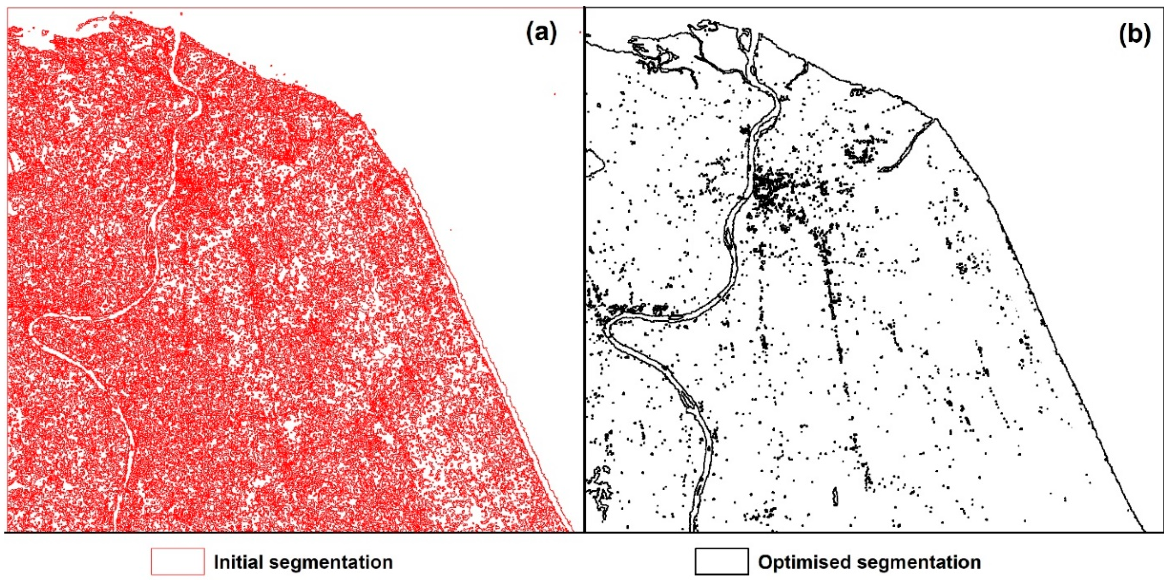
After numerous experiments in this stage, the optimal result for the imagery was achieved when the scale and maximum spectral difference values were 50, the shape and compression parameters were 0.9 and the chessboard value was 20 (Table 5). Figure 8 shows the segmentation result based on the selected parameters. Defining the ideal segmentation threshold is one of the main steps in our model towards automation, which can be applied on similar environment and climate to accurately classify land from water. The optimisation process on different imageries and conditions is subjected to size, pattern and tone of environmental features.

The size of polygon boundaries indicates the result of segmentation (Figure 8). The initial segmentation results that came from basic MSA, maximum spectral difference and chessboard segmentation methods showed too many unessential segments, particularly in land and shoreline border. The feature classes, such as water and land, could not be separated accurately using the initial segmentation result; therefore, shoreline border identification was also not precise (Figure 8a). However, after optimising the segmentation parameters, the segments were well defined. The fittest segments for features (e.g., land and water) on the images were generated due to the optimal selection of the scale, shape, compactness, spectral difference and chessboard values. This optimised method could remove the unessential and small segments that caused uncertainty in classification (Figure 8b). The optimised segmentation helped the SVM classifier gain a consistent classified map.

3.2. SAR Classification Results

When the sample size in each individual class was less than 25, the accuracy of the classes was unsatisfactory. When the sample size increased to 80, the highest accuracy in classification was obtained. The SVM uses support vectors instead of all the training protocols to make the isolation hyperplane. Therefore, the number of training samples may affect the classification accuracy. In the current experiment, a sample size of 80 in each class was considered ideal; beyond this value, size would not essentially lead to a considerable increase in the degree of accuracy of the classification.

The 2003 classified map was assessed by 30 ground control points (GCPs) for each class that distributed randomly all over the scene. These GCPs were collected from a classified Landsat image in November 2003. On the contrary, the 2014 classified map was assessed by 30 GCPs for each class that were collected from Digital Globe imagery (Google Earth) on November 2014. A reliable thematic map with the highest overall classification accuracy was used as the reference to determine the exact accuracy of the implemented classification [35,36]. We stratified randomly selected sample training and experimentation for both images to evaluate overall accuracy of classification with optimal parameter values (

Table 6. Comparison of the overall accuracy result.

SAR Images	SVM Classifier Accuracy
2003	98.3%
2014	98.7%

). On the basis of the error matrix of the thematic maps, we calculated Z-statistics to assess the difference in the results of the classification between the two categories [37].

3.3. Quantitative Assessment of Detected Changes

Frequent shoreline monitoring and accurate change detection are vital for understanding coastal procedures and various dynamics of the coastal characteristics. Coastal position is an important geographical indicator in coastal development and provides useful information on the dynamics of coastal morphology [38]. Therefore, accurate detection and monitoring of the coastal area are essential for recognising coastal processes and the dynamics of various coastal characteristics.

A quantitative assessment of the metrics and pattern of temporal shoreline dynamics should be applied on specific transects on the shoreline retrieved from the RADARSAT images. Area and length of shorelines were measured to indicate the magnitude of shoreline temporal changes (

Table 7. Quantitative assessment of morphology of the shoreline dynamic.

Transect	Onshore Changes (Erosion)	Offshore Changes (Accretion)	No Changes
I	105.97 ha	248.21 ha	1094.34 ha
	7.3%	17.4%	75.6%
II	12.47 ha	115.60 ha	648.68 ha
	1.6%	14.9%	83.5%
III	77.66 ha	48.07 ha	645.41 ha
	10.1%	6.2%	83.7%
IV	13.67 ha	21.34 ha	533.65 ha
	2.4%	3.8%	93.8%
V	4.21 ha	20.23 ha	579.88 ha
	0.7%	3.3%	96.0%
VI	13.47 ha	1.77 ha	402.82 ha
	3.1%	0.4%	96.5%

).

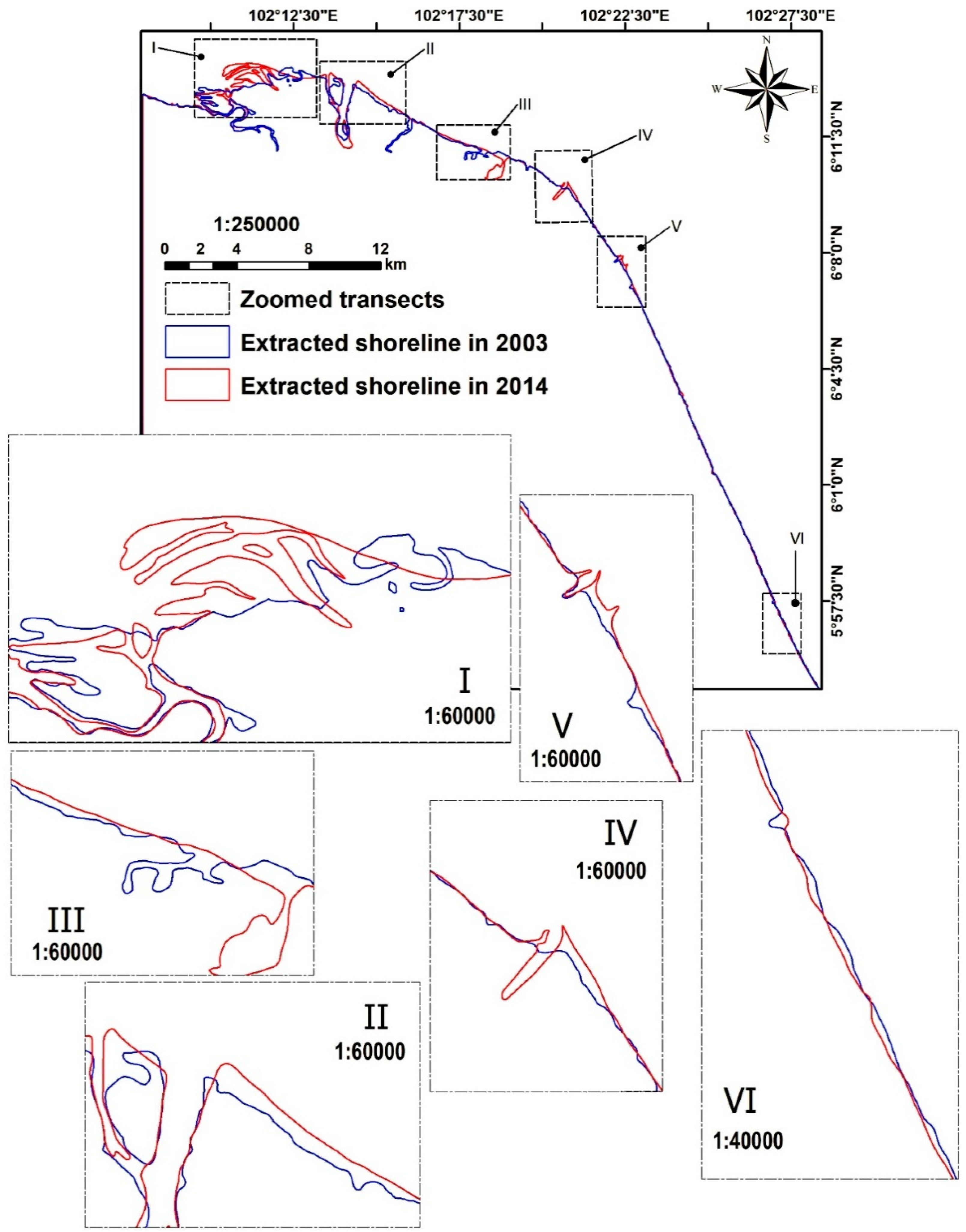
The changes were calculated by measuring the observed distances between the shorelines of 2003 and 2014. Notably, the shoreline had shifted towards the northeast and had slightly shifted to the southeast side of the coast by 12.8 m in average (Figure 9). Considering the shoreline morphological pattern, the shoreline in 2003 was straighter than the shoreline in 2014. Overall, the coastal length increased from 101.50 km to 115.22 km during the period of 2003 to 2014. To be more specific, the change detection analysis was conducted in six transects in which it had experienced significant changes. In each transect, the magnitude of the changed area was measured on the basis of onshore, offshore and no changes calculation. Onshore changes reflect the movement of the sea towards land, causing erosion. However, offshore changes happen where the sea is pushed back from land, resulting in accretion.

During the given period, the shoreline experienced less dynamics in transects VI and V where 96.5 and 96.0 percentage of shoreline remains unchanged, respectively. Particularly, the shoreline in transect I and nearby areas had not changed remarkably. However, most changes had occurred in transect I where just 75.6% of shoreline area remained unchanged. In transect I, almost 248 hectares were added to shore areas, while 106 hectares were removed from shore area from 2003 to 2014. Basically, the onshore and the offshore variation were noticeable in all the measured transects. In transect VI and III, the number of offshore change was more than other transects (i.e., 0.4 and 0.6 percentage), which indicated the eroded shoreline. In transects I, II, IV and V, offshore change was detected more than onshore change (Table 7).

3.4. Validation

The delineated 2003 shoreline was validated by overlaying the surveyed shoreline from JUPEM, while the delineated 2014 shoreline was validated by Digital Globe satellite imagery from Google Maps. The referenced images provided details on the area and position information over the area, such as the coordinate. Accordingly, we compared this shoreline with the extracted shoreline for accuracy assessment. Comparison analysis of the extracted shoreline with the referenced shorelines were placed in 32 random, well-distributed transects along the border for 2003 and 2014 (

Table 8. Validation of SAR-extracted shorelines with references.

Compared Distance Statistics	Year
	2003	2014
Minimum:	0.22 (m)	0.00 (m)
Maximum:	7.85 (m)	6.13 (m)
Mean:	2.56 (m)	1.97 (m)
Standard Deviation:	1.69 (m)	1.35 (m)

).

In 2003, the recorded minimum distance between both shorelines was 0.22 m, whereas the maximum drift was 7.85 m. The average distance of differential for every point was 2.56 m. The range of differences was up to 1.69 m. In 2014, the recorded minimum distance between both shorelines was zero metre, whereas the maximum drift was 6.13 m. The average distance of differential for every point was 1.35 m. The range of differences was up to 1.69 m. The validation results showed a considerable correlation between referenced shorelines and extracted ones. However, in 2014, we observed high similarity between the two shorelines that might be due to the higher quality of RADARSAT-2 compared to the first product of RADARSAT.

After validation analysis, the final shoreline border of 2014 was calibrated. From the observation and analysis, we found that accurate measurement of the differences needed to be quantified using approximately the same level of the tidal condition in the identified shoreline.

4. Discussion

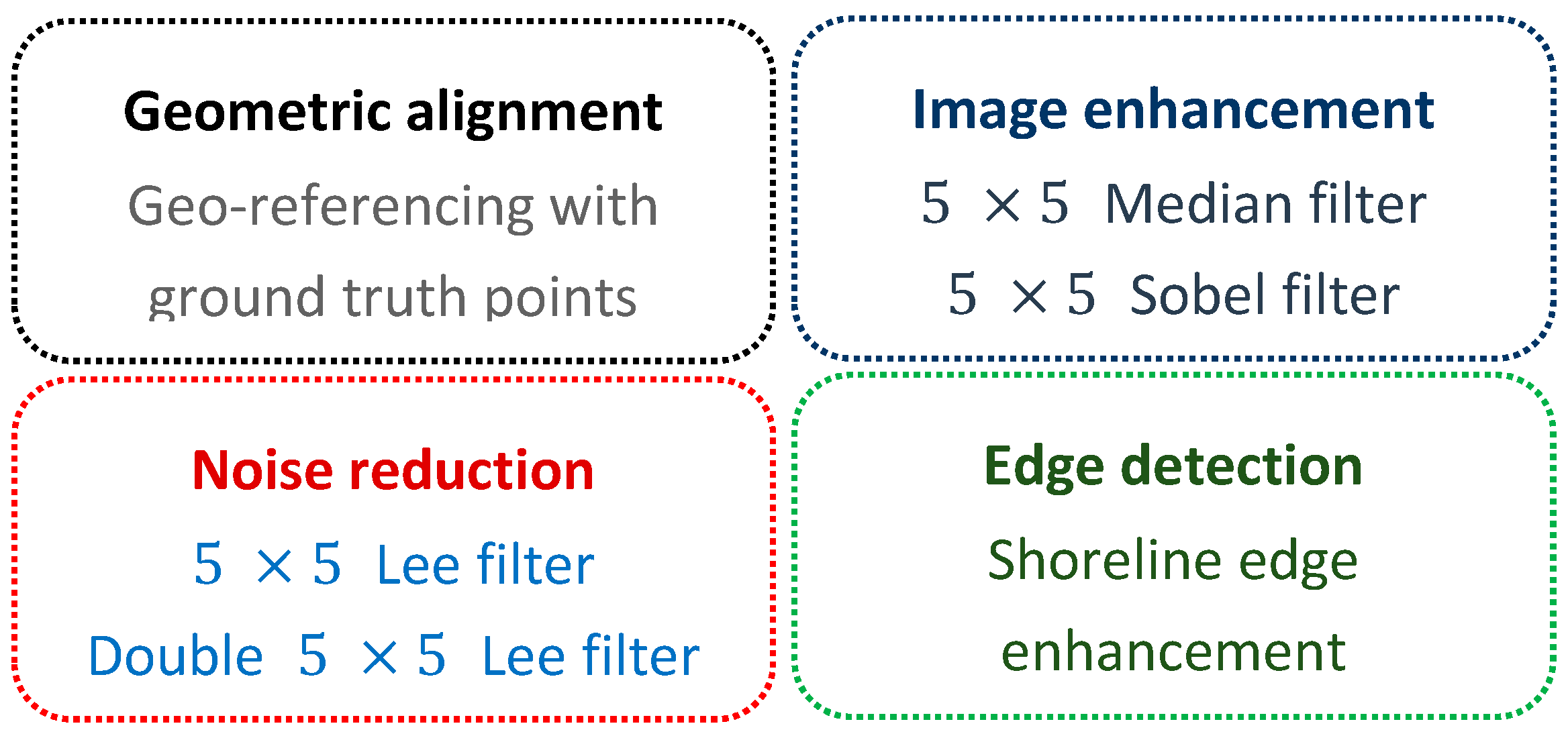
A coastline is an intersection between the midline of the water and the coast. The line that divides the coastline into marine charts is nearly a moderate line [39]. Coastlines have fast-changing nature. Thus, proper definition of coastline change is important for identification of county boundary, navigation and shoreline matters. SAR imagery (e.g., RADARSAT-1 and RADARSAT-2) is a valuable dataset for detection and description of coastlines. In general, extraction and recognition of coastal features from SAR images involve a series of practices, including filtering, progression, image segmentation, shoreline extraction and change detection. In this study, a semiautomated process was created to monitor the shifts and extraction of the coastline of Kelantan, Malaysia, from RADARSAT. This proposed process is an advanced technique for radar images. A system of different segmentation analyses was applied to the filtered images to separate the land and ocean. After the segmentation result was obtained, assessment of changes was conducted using an SVM classifier to achieve improved classification result. The results revealed that SVM provided overall accuracies of 98.7% and 98.3% on images in 2003 and 2014, respectively. To substantiate the accuracy of SVM classifier, two other classifier methods, namely, k-nearest neighbours (k-NN) and decision tree (DT), were applied on both SAR imageries. The comparison results of classified maps with GCPs showed that SVM generally had the best performance among the three classifiers with the optimal parameter setting; the minimum overall accuracy of SVM was 98.34%, which was higher than the maximum overall accuracy of DT (94.2%) and k-NN (96.6%). The high-performance classifier was used in further processing to derive the final shoreline. The SVM classifier is less sensitive to sample sizes because SVM only uses the support vectors instead of all training samples to build the separating hyperplane. Thus, adding a large number of training samples would not considerably affect the classification accuracy, in which the increase in sample size does not necessarily lead to a considerable increase in classification accuracies. In this study, we tried to increase the number of training samples as much as possible. However, the result of classification was not enhanced when the number of training samples was 80. When training samples of 90 and 100 were tested for each class of land use in 2014, the classification accuracy dropped to 97.3% and 97.1%, respectively.

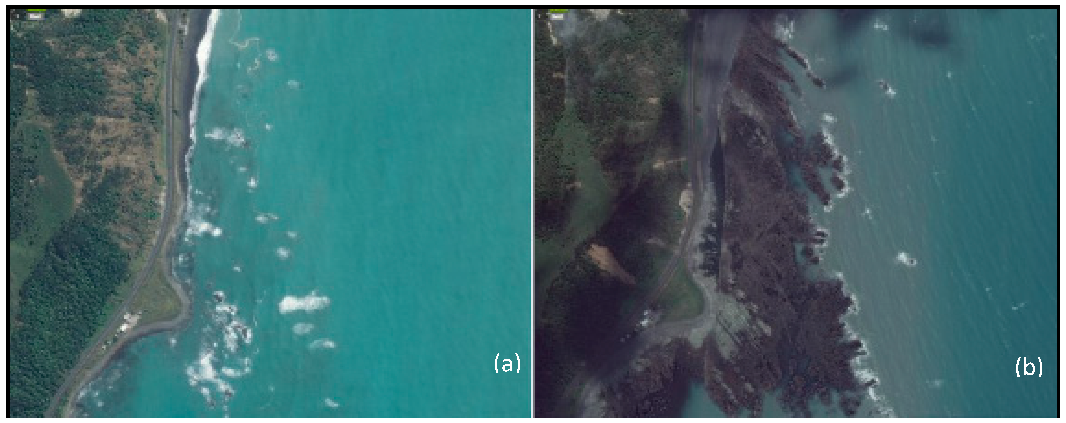
Distortions were shown in some locations, which may be attributed to the changes in the coastline over the years due to the impact of tsunami; these changes might have affected the shifted shoreline of Kelantan (Figure 10). The 2004 Indian Ocean earthquake with the magnitude of 9.1 to 9.3 (Mw) caused the tsunami to collapse along the coast of Pahang and Kelantan, thereby shifting them from a few metres to many hundred metres inland [40].

Wet sands on the beach are a source of uncertainty for SAR image classification. Thus, they must be considered in the process. Some sandy areas become wet due to tidal phenomena. This condition can cause the distortion on the backscatter coefficient for the spectral difference segmentation in separating land and ocean. Therefore, the date of image capturing should be synchronised on multitemporal images when similar tidal level occurs on the sandy beach. A previous study estimated that the coast is raised between 0.5 and 2 m from approximately 20 km in the south of Kaikoura [41].

Shoreline changes are usually influenced by cross-shore sediment transport processes and human interferences. However, tsunamis and earthquakes considerably impact shoreline changes. In the validation analysis, the average differences between the SAR shoreline and the surveyed shoreline were 2.56 and 1.97 m for 2003 and 2014, respectively. A total of 32 randomly transects were measured to calculate the validation parts, although the remaining points along the shoreline borders were visually fitted on the intersection of one another in the two approaches. The visual interpretation showed that the major coastline shift had occurred in the northeast side of the coast between 2003 and 2014 during which the coastal movement was towards the ocean. The southeast part of the shoreline had also shifted slightly compared with the northeast part.

5. Conclusions

A semiautomatic methodology for detecting shorelines using single SAR images is a powerful method to extract coastlines for mapping purpose. Coastal surveying and detection are crucial for environmental protection and sustainable coastal zone management. This paper describes a simple and effective algorithm for detecting coastlines. An optimised technique for SAR image preprocessing, segmentation and classification was proposed to detect shoreline dynamics. After coastline detection, coastline extraction was achieved using a fast and reliable segmentation technique to delineate shoreline information. SAR imagery has a high capability to extract shorelines in tropical regions under cloud coverage. The results showed that the applied method had a high degree of accuracy based on the validation of the surveyed thematic map. Ideally speaking, for an accurate change detection result using multitemporal dataset, satellite images should be captured at the same date and time of the years, with similar atmospheric condition and tide level.

The change detection results showed an average difference in the shoreline by 12.5 m between 2003 and 2014. A comparison of the extracted shoreline with the coastline drawn by JUPEM and Digital Globe satellite image revealed general similarities in coastline curvature. Misrepresentations were also shown in some places, and they might be due to coastal changes over the years because of the effects of tsunami and earthquakes. The proposed methods and procedures can identify and map coastlines for updating the geographic charts and other maps required for accurate coastal mapping. Further works should use drone-based technologies and high-resolution satellite imagery for accurate coastline detection and monitoring. Comprehensive and detailed in situ tidal variation data and land use/land cover patterns should also be considered in future studies.

References

1. Alesheikh, A.A.; Ghorbanali, A.; Nouri, N. Coastline change detection using remote sensing. Int. J. Environ. Sci. Technol. 2007, 4, 61–66. [Google Scholar] [CrossRef] [Green Version]
2. Natesan, U.; Parthasarathy, A.; Vishnunath, R.; Kumar, G.E.J.; Ferrer, V.A. Monitoring longterm shoreline changes along Tamil Nadu, India using geospatial techniques. Aquat. Procedia 2015, 4, 325–332. [Google Scholar] [CrossRef]
3. Billa, L.; Pradhan, B. Semi-automated procedures for shoreline extraction using single RADARSAT-1 SAR image. Estuar. Coast. Shelf Sci. 2011, 95, 395–400. [Google Scholar]
4. Olthof, I.; Tolszczuk-Leclerc, S. Comparing Landsat and RADARSAT for Current and Historical Dynamic Flood Mapping. Remote Sens. 2018, 10, 780. [Google Scholar] [CrossRef]
5. Schulze, M.A.; Wu, Q.X. Noise reduction in synthetic aperture radar imagery using a morphology-based nonlinear filter. In Proceedings of the DICTA95, Digital Image Computing and Applications, Brisbane, Australia, 6–8 December 1995. [Google Scholar]
6. Herold, N.D.; Haack, B.N.; Solomon, E. An evaluation of radar texture for land use/cover extraction in varied landscapes. Int. J. Appl. Earth Obs. Geoinf. 2004, 5, 113–128. [Google Scholar] [CrossRef]
7. Marghany, M.; Hashim, M. Developing adaptive algorithm for automatic detection of geological linear features using RADARSAT-1 SAR data. Int. J. Phys. Sci. 2010, 5, 2223–2229. [Google Scholar]
8. Pradhan, B. Remote sensing and GIS-based landslide hazard analysis and cross-validation using multivariate logistic regression model on three test areas in Malaysia. Adv. Space Res. 2010, 45, 1244–1256. [Google Scholar] [CrossRef]
9. Schowengerdt, R.A. Remote Sensing: Models and Methods for Image Processing; Elsevier: Amsterdam, The Netherlands, 2006. [Google Scholar]
10. Manca, E.; Pascucci, V.; Deluca, M.; Cossu, A.; Andreucci, S. Shoreline evolution related to coastal development of a managed beach in Alghero, Sardinia, Italy. Ocean Coast. Manag. 2013, 85, 65–76. [Google Scholar] [CrossRef]
11. Mahmoud, A.; Elbialy, S.; Pradhan, B.; Buchroithner, M. Field-based landcover classification using TerraSAR-X texture analysis. Adv. Space Res. 2011, 48, 799–805. [Google Scholar] [CrossRef]
12. Chaaban, F.; Darwishe, H.; Louche, B.; Battiau-Queney, Y.; Masson, E.; el Khattabi, J.; Carlier, E. Geographical information system approach for environmental management in coastal area (Hardelot-Plage, France). Environ. Earth Sci. 2012, 65, 183–193. [Google Scholar] [CrossRef]
13. Rizeei, H.M.; Pradhan, B. Extraction and accuracy assessment of DTMs derived from remotely sensed and field surveying approaches in GIS framework. In IOP Conference Series: Earth and Environmental Science; IOP Publishing: Bristol, UK, 2018. [Google Scholar]
14. Chen, L.; Shyu, C. Automated extraction of shorelines from optical and SAR images. In Proceedings of the 19th Asian Conference on Remote Sensing, Manila, Philippines, 16–20 November 1998; Available online: http://www. gisdevelopment. net/aars/acrs (accessed on 29 October 2018).
15. Henderson, F.M.; Lewis, A.J. Principles and applications of imaging radar. Man. Remote Sens. 1998, 2. [Google Scholar]
16. Marghany, M.; Hashim, M.; Cracknell, A. Simulation of shoreline change using AIRSAR and POLSAR C-band data. Environ. Earth Sci. 2011, 64, 1177–1189. [Google Scholar] [CrossRef]
17. Biro, K.; Pradhan, B.; Buchroithner, M.; Makeschin, F. Land use/land cover change analysis and its impact on soil properties in the northern part of Gadarif region, Sudan. Land Degrad. Dev. 2013, 24, 90–102. [Google Scholar] [CrossRef]
18. Waring, R.H.; Way, J.; Hunt, E.R.; Morrissey, L.; Ranson, K.J.; Weishampel, J.F.; Oren, R.; Franklin, S.E. Imaging radar for ecosystem studies. BioScience 1995, 45, 715–723. [Google Scholar] [CrossRef]
19. Xiao, J.; Li, J.; Moody, A. A detail-preserving and flexible adaptive filter for speckle suppression in SAR imagery. Int. J. Remote Sens. 2003, 24, 2451–2465. [Google Scholar] [CrossRef]
20. Lee, J.-S.; Jurkevich, I. Coastline detection and tracing in SAR images. IEEE Trans. Geosci. Remote Sens. 1990, 28, 662–668. [Google Scholar]
21. Choi, J.-K.; Oh, H.-J.; Koo, B.J.; Ryu, J.-S.; Lee, S. Spatial polychaeta habitat potential mapping using probabilistic models. Estuar. Coast. Shelf Sci. 2011, 93, 98–105. [Google Scholar] [CrossRef]
22. Jose, A.; Dixon, K.D.M.; Joseph, N.; George, E.S.; Anjitha, V. Performance study of edge detection operators. In Proceedings of the 2014 International Conference on Embedded Systems (ICES), Coimbatore, India, 3–5 July 2014. [Google Scholar]
23. Parker, J.R. Algorithms for Image Processing and Computer Vision; John Wiley & Sons: Hoboken, NJ, USA, 2010. [Google Scholar]
24. Liu, H.; Jezek, K. Automated extraction of coastline from satellite imagery by integrating Canny edge detection and locally adaptive thresholding methods. Int. J. Remote Sens. 2004, 25, 937–958. [Google Scholar] [CrossRef]
25. Jia, X.; Richards, J.A. Segmented principal components transformation for efficient hyperspectral remote-sensing image display and classification. IEEE Trans. Geosci. Remote Sens. 1999, 37, 538–542. [Google Scholar]
26. Blaschke, T.; Hay, G.J.; Kelly, M.; Lang, S.; Hofmann, P.; Addink, E.; Feitosa, R.Q.; Van der Meer, F.; Van der Werff, H.; Van Coillie, F.; et al. Geographic object-based image analysis–towards a new paradigm. ISPRS J. Photogramm. Remote Sens. 2014, 87, 180–191. [Google Scholar] [CrossRef] [PubMed]
27. Mojaddadi, H.; Pradhan, B.; Saharkhiz, M.A. Urban object extraction using Dempster Shafer Feature Based Image Analysis from Worldview-3 satellite imagery. Int. J. Remote Sens. 2018, 1–28. [Google Scholar] [CrossRef]
28. Wieland, M.; Pittore, M. Performance evaluation of machine learning algorithms for urban pattern recognition from multi-spectral satellite images. Remote Sens. 2014, 6, 2912–2939. [Google Scholar] [CrossRef]
29. Aal-shamkhi, A.D.S.; Mojaddadi, H.; Pradhan, B.; Abdullahi, S. Extraction and modeling of urban sprawl development in Karbala City using VHR satellite imagery. In Spatial Modeling and Assessment of Urban Form; Springer: Berlin, Germany, 2017; pp. 281–296. [Google Scholar]
30. Rizeei, H.M.; Shafri, H.Z.; Mohamoud, M.A.; Pradhan, B.; Kalantar, B. Oil palm counting and age estimation from WorldView-3 imagery and LiDAR data using an integrated OBIA height model and regression analysis. J. Sens. 2018, 2018. [Google Scholar] [CrossRef]
31. Taguchi, G. Introduction to Quality Engineering: Designing Quality into Products and Processes; Quality Resources: Linkedin, CA, USA, 1986. [Google Scholar]
32. Pradhan, B. Landslide susceptibility mapping of a catchment area using frequency ratio, fuzzy logic and multivariate logistic regression approaches. J. Indian Soc. Remote Sens. 2010, 38, 301–320. [Google Scholar] [CrossRef]
33. Dell’Acqua, F.; Gamba, P. Rapid mapping using airborne and satellite SAR images. In Radar Remote Sensing of Urban Areas; Springer: Berlin, Germany, 2010; pp. 49–68. [Google Scholar]
34. Blanchard, S.D.; Jakubowski, M.K.; Kelly, M. Object-based image analysis of downed logs in disturbed forested landscapes using lidar. Remote Sens. 2011, 3, 2420–2439. [Google Scholar] [CrossRef]
35. Abdullahi, S.; Pradhan, B.; Mojaddadi, H. City compactness: Assessing the influence of the growth of residential land use. J. Urban Technol. 2018, 25, 21–46. [Google Scholar] [CrossRef]
36. Nampak, H.; Pradhan, B.; Rizeei, H.M.; Park, H.J. Assessment of land cover and land use change impact on soil loss in a tropical catchment by using multitemporal SPOT-5 satellite images and R evised U niversal Soil L oss E quation model. Land Degrad. Dev. 2018. [Google Scholar] [CrossRef]
37. Song, X.; Duan, Z.; Jiang, X. Comparison of artificial neural networks and support vector machine classifiers for land cover classification in Northern China using a SPOT-5 HRG image. Int. J. Remote Sens. 2012, 33, 3301–3320. [Google Scholar] [CrossRef]
38. Maiti, S.; Bhattacharya, A.K. Shoreline change analysis and its application to prediction: A remote sensing and statistics based approach. Mar. Geol. 2009, 257, 11–23. [Google Scholar] [CrossRef]
39. Boak, E.H.; Turner, I.L. Shoreline definition and detection: A review. J. Coast. Res. 2005, 21, 688–703. [Google Scholar] [CrossRef]
40. Suppasri, A.; Koshimura, S.; Matsuoka, M.; Gokon, H.; Kamthonkiat, D. Application of remote sensing for tsunami disaster. In Remote Sensing of Planet Earth; InTech: London, UK, 2012. [Google Scholar]
41. Barnes, P.; Mountjoy, J.; Wilcox, S.; Mitchell, S.; Pallentin, A.; Amyes, D. National Institute of Water and Atmospheric Research (NIWA) Voyage Report, Ocean 2020 Northern Hikurangi Margin Geohazards; RV Tangaroa Rep. Tan1114; NIWA: Wellington, New Zeland, 2011. [Google Scholar]
Figure 1. Geographical location of the study area in Malaysia.
Remotesensing 10 01705 g001
Figure 2. (a) RADARSAT-2 and (b) RADARSAT-1 showing delta area of Kota Bharu District.
Remotesensing 10 01705 g002
Figure 3. Computational workflow applied in this study.
Remotesensing 10 01705 g003
Figure 4. Preprocessing methods applied in this research.
Remotesensing 10 01705 g004
Figure 5. Visualisation of noise reduction using (a) single and (b) double Lee filters.
Remotesensing 10 01705 g005
Figure 6. Image enhancement using different designs of Sobel templates: (a) horizontal and (b) vertical kernels.
Remotesensing 10 01705 g006
Figure 7. Median and Sobel filters with a kernel size of   5 × 5 .
Remotesensing 10 01705 g007
Figure 8. Segmentation results. (a) initial segmentation; and (b) optimized segmentation.
Remotesensing 10 01705 g008
Figure 9. Shoreline changes from 2003 to 2014.
Remotesensing 10 01705 g009
Figure 10. Waipapa Bay’s shoreline changes (a) before (b) and after tsunami captured by WorldView-2 images. (Source: http://info.geonet.org.nz).
Remotesensing 10 01705 g010