Abstract
Deep-seated gravitational slope deformations (DSGSDs) endanger settlements and infrastructure in mountain areas all over the world. To prevent disastrous events, their activity needs to be continuously monitored. In this paper, the movement of the Reissenschuh DSGSD in the Schmirn valley (Tyrol, Austria) is quantified based on point clouds acquired with a Riegl VZ®-6000 long-range laser scanner in 2016 and 2017. Geomorphological features (e.g., block edges, terrain ridges, scarps) travelling on top of the landslide are extracted from the acquired point clouds using morphometric attributes based on locally computed eigenvectors and -values. The corresponding representations of the extracted features in the multi-temporal data are exploited to derive 3D displacement vectors based on a workflow exploiting the iterative closest point (ICP) algorithm. The subsequent analysis reveals spatial patterns of landslide movement with mean displacements in the order of 0.62 ma, corresponding well with measurements at characteristic points using a differential global navigation satellite system (DGNSS). The results are also compared to those derived from a modified version of the well-known image correlation (IMCORR) method using shaded reliefs of the derived digital terrain models. The applied extended ICP algorithm outperforms the raster-based method particularly in areas with predominantly vertical movement.
1. Introduction
Deep-seated gravitational slope deformations (DSGSDs) pose a serious threat to settlements and infrastructure in mountain regions all over the world. Therefore, their spatial extent must be assessed and their activity needs to be monitored. Various monitoring techniques can be used to quantify landslide movement at characteristic points, along profiles or area-wide. Measurement techniques at points include (i) continuous or periodical measurements with a differential global navigation satellite system (DGNSS) [1,2], (ii) geodetic techniques using a tachymeter or a level [3,4] and (iii) techniques for measuring distances such as laser distance meters or wire extensometers [5,6]. Monitoring techniques applicable along profiles include (i) indirect, geophysical measurements [7,8] and (ii) direct measurements e.g., by using inclinometers [9,10]. Only remote sensing techniques—collecting information about an object without physical contact [11]—can provide an area-wide coverage of an area of interest. In several studies, the movement of DSGSDs has been assessed using various kinds of sensors and techniques, including (i) space-born differential synthetic aperture radar interferometry (DInSAR) [12,13] as well as ground-based DInSAR [14,15], (ii) terrestrial laser scanning (TLS) [16,17], (iii) airborne laser scanning (ALS) [18,19] and (iv) photogrammetric techniques [20,21].
The application of DInSAR for landslide monitoring implies limitations on the displacement rate and direction. Furthermore, this technique depends on the characteristics of the illuminated surface and is particularly limited in vegetated areas [22]. Photogrammetric techniques typically rely on imagery acquired from unmanned aerial vehicle (UAV) or terrestrial platforms. Because of limitations regarding the range and spatial coverage of these acquisition techniques, landslide monitoring based on photogrammetrically derived point clouds from UAV and terrestrial platforms is usually restricted to small areas of interest [23]. TLS is a cost-effective technique for monitoring landslide displacements in a mountain environment. It provides an efficient data acquisition with area-wide coverage and high measurement precision (in the order of 10 centimetres) [24,25]. An advantage of this technique is that it can penetrate (high) vegetation and deliver terrain models representing the terrain surface after filtering, allowing to assess changes of the ground also under forest cover [26].
So far, there is no clear definition of close-range and long-range TLS. The terms ’long-range’, ’very-long-range’ and ’ultra-long-range’ were used in previous studies with maximum scanning distances of 800 to 6000 [27,28,29,30]. Compared to close-range TLS, long-range TLS (LRTLS) faces challenges which emerge due to the long scanning distance. Associated phenomena are larger footprints due to the widening of the laser beam and atmospheric influences affecting the distance estimation as well as an inhomogeneous point density throughout the area of interest. Hence, also the measurement accuracy and the detectability of objects and features decreases with increasing scanning distance [25]. Nevertheless (LR)TLS is an efficient technique frequently used in Geoscience for acqquiring high-resolution 3D point clouds of the earth surface. For landslide monitoring, TLS is typically applied to derive multi-temporal point clouds for quantifying surface and volume changes i.e., deformation and displacement rates in multi-temporal data where geologic and geomorphologic processes occur in a certain frequency-magnitude relation [31,32]. Change detection and deformation studies based on TLS have been conducted already a decade ago demonstrating the advantage of area-wide high-resolution data sets detecting changes and estimating accuracies by comparing TLS data with GNSS and tachymeter measurements [33,34]. However, an ongoing important key question is the reliable estimation of error budgets in real world open lab setups in order to determine which changes are due to real mass movement and which ones do occur due to the measurement principle itself considering sensor characteristics, measurement setup, and environmental conditions [25,35,36]. Ongoing research focuses on optimizing measurement setups, minimizing registration errors, automating registration [37] and automating change detection for interpreting landslide induced surface changes [38,39].
Object-based monitoring approaches allow a more detailed analysis of changes on landslide substructures [39]. Object-based tracking of displacements may be helpful in cases where velocities, surface structure and vegetation do not allow the application of common raster-based correlation methods [17]. In such cases the derivation of displacement vectors from particular geomorphological structures are promising concepts for detailed interpretation of landslide activity and displacement patterns as limitations related to raster size and the applied raster aggregation method can be avoided. Furthermore, displacement can be quantified in 3D using point clouds whereas raster-based approaches work with 2D maps or 2.5D elevation models.
The objectives and aims presented in this paper are
- the automated extraction of geomorphological features,
- to establish point neighbourhood correspondences in the multi-temporal data,
- to derive significant displacements well above the uncertainty of the acquired point cloud data and
- to compare the results of the applied method to those of a state-of-the-art raster-based change detection method.
Displacements of a DSGSD located in the Schmirn valley (Tyrol, Austria) are assessed by analyzing multi-temporal data acquired with a differential global navigation satellite system (DGNSS) and a long-range terrestrial laser scanner. From the acquired point clouds, 3D-displacement vectors are derived from extracted geomorphological features travelling on top of the landslide. The DGNSS measurements, featuring a higher accuracy, serve for validation purposes of the magnitude and direction of the landslide displacements derived from LRTLS. Particular attention is paid to the error budget resulting from inherent uncertainties of both monitoring methods. For the area-wide derivation of 3D displacement vectors an extended version of the well-known iterative closest point (ICP; [40]) algorithm is used. Its results are compared with those of an modified image correlation technique (IMCORR; [41]).
2. Study Area
The monitored DSGSD is situated on a south-facing slope of the east-west striking Schmirn valley in Tyrol, Austria (Figure 1a). It is located below the summit of the Reissenschuh (2470 ) and is surrounded by a mountain range with heights up to 2600 in the west, north and east. The present active part of the Reissenschuh landslide covers altitudes between 1700 and 2300 .
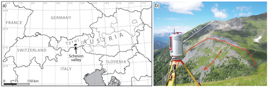
Figure 1.
Location of the study area (a) in the Schmirn valley and (b) photo of the Reissenschuh DSGSD from the opposite valley flank. Photo: J. Pfeiffer, 28 June 2016.
The geological substratum around the Reissenschuh DSGSD is characterized by lithologies of the subpenninic nappe of the Tauern Window. The geological predisposition of the landslide is given by relatively competent permeable marble containing mica-calcareous phyllites and schists overlaying soft, incompetent, clayey weathering and impermeable black phyllites [42]. Furthermore, a well developed set of discontinuity related to the foliation dipping with 30 towards north and sub-vertical, mostly opened, joints are apparent.
The mean annual precipitation sum recorded on the valley floor at the meteorological station in Toldern (1461 ) is around 1000 mm with a maximum during the summer months. The mean annual air temperature at Toldern station is . During the winter months the mean air temperature drops distinctly below zero, facilitating the accumulation of considerable amounts of snow. In late spring snow melt and the infiltrating meltwater may cause higher pore pressures which could lead to enhanced landslide activity.
In the Schmirn valley meadows and pasture are the dominant land use types on the valley floor and adjacent slopes. Steeper slopes are covered by forest, mainly composed of larch (Larix decidua Mill.) and spruce (Picea abies L. Karsten). At higher altitudes the forest gets sparser while the proportion of larch increases. Above an altitude of about 2000 the land cover is dominated by low vegetation such as Alpine rose (Rhododendron hirsutum L.), mountain pine (Pinus mugo L.) or Alpine meadows used for sheep pasture. Part of the presently active landslide is covered by a sparse larch forest and mountain meadow with mountain roses and other scrub plants.
3. Materials and Methods
3.1. Differential Global Navigation Satellite System
The spatio-temporal activity of the Reissenschuh landslide was monitored at points with the help of a DGNSS. On top of 28 boulders distributed all over the study area, surveying nails were installed. Large boulders of at least 1 in size were selected, all located above the tree line or within clearances to prevent multipath effects during the DGNSS measurements. In case boulders were not properly embedded within the soil matrix, up to three surveying nails were installed to assess effects of eventually rotating movements. The positions of the nails were measured several times a year, using a Trimble Geo7 receiver with a Zephyr antenna mounted on top of a 2 pole. During the measurements of at least five minutes, the pole was fixed upright with a tripod. The measurement device can handle the signals of several GNSS systems, including GPS, GLONASS, GALILEO and BEIDOU. The phase and precise code of both carrier frequencies in the L-band (L1 and L2) of available GPS and GLONASS satellites were recorded. All measurements were corrected in the post-processing, using simultaneously recorded data from a close permanent GNSS station located in Sterzing (Italy), about 16 km from the study area. This station is operated by the South Tyrolean Positioning Service (STPOS), providing continuous data with a temporal resolution of one second. The resulting uncertainty of the corrected data is in the range of cm to cm, depending on the number of available satellites and their geometric constellation during the measurements. After the post processing, the magnitude and direction of the landslide-induced displacement was derived from the multi-temporal DGNSS measurements. The results provide data for validating the displacements derived from the multi-temporal LRTLS measurements.
3.2. Long-Range Terrestrial Laser Scanning
A Riegl VZ®-6000 long-range terrestrial laser scanner was used to acquire 3D point clouds of the DSGSD on 28 June 2016 and 26 June 2017. The scanner operates with a wavelength of 1064 nm. It features a class 3B laser which requires precautions in terms of eye safety. Scanning frequencies were set to 150 kHz and column and line resolutions of to and to respectively, resulting in individual point clouds with up to 395 million points with an average 2D point spacing of about 5 cm. To minimize the potential uncertainty caused by atmospheric influences, meteorological data from a nearby meteorological station were considered during the registration of the point clouds. Further methods of data processing are summarized in Figure 2a and also described in more detail in the following. The Riegl RiScan Pro software [43] was used for the recalculation and separation of multiple echos in the air (MTA). All further processing steps such as point cloud registration, ground filtering, raster aggregation, shaded relief creation, curvature calculation, breakline extraction and displacement vector derivation were conducted with the SAGA LIS software [44]. For classifying ground and non-ground points the triangular irregular network (TIN) densification approach proposed by [45] was applied.
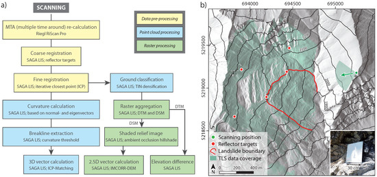
Figure 2.
Processing steps and field setup. (a) Workflow, methods and used software for processing the LRTLS data and (b) field setup of the LRTLS acquisitions. The photo in the lower right corner shows a reflector target installed in the study area. The map is shown in the UTM 32N projection (EPSG-Code: 25832). Photo: J. Pfeiffer, 10 June 2016.
3.3. LRTLS Accuracy Estimation
Prior to the point cloud acquisition the expected measurement accuracy and the associated detection threshold were estimated, allowing to differentiate between real landslide-induced changes and data noise. Particularly the unknown atmospheric conditions prevailing in the study area can have adverse effects on the distance estimation [46]. For the correction of atmospheric influences average values of temperature, air pressure and humidity were used. These parameters underlie considerable spatio-temporal variability especially in mountain regions and consequently lead to uncertainties in the distance estimation. Following [47], the distance [m] is derived from
where [s] is the time of flight, c ( ms) is the speed of light and n is the atmospheric refraction index. Subsequently, the refraction index depends on the wavelength of the sensor and on the prior described varying atmospheric conditions that are temperature, pressure and humidity. Increasing measurement distance and atmospheric differences between scan position and measured surface result in higher uncertainties of distance estimation if just one atmospheric correction index n is applied for the whole dataset. Determination of a maximum and minimum possible atmospheric refraction index that might occur distributed over the investigation area allow a quantification of the potential atmospheric uncertainty. Based on the local conditions a maximum atmospheric uncertainty of up to cm at a maximum measurement distance of 2500 and altitude change of 1200 is considered for further data processing.
Due to the divergence of the laser beam ( 0.12 mrad in case of the Riegl VZ®-6000), the footprint size increases with the measurement distance [47,48]. Maximum measured distance within the study area of about 2500 , a 30 cm footprint diameter can be expected on a surface normal to the laser beam axis, considering a Gaussian beam with its footprint radius defined at irradiance. Perpendicular conditions create a footprint with the geometry of a circle. Inclined impact conditions modify the circle geometry to a larger, ellipsoidal footprint. Since there is no clear spatial definition of where the reflected signal was generated within the projected footprint, the whole footprint should be considered as a potential range of uncertainty [49]. Assuming planar and spectral homogeneous surfaces at appropriate footprint scale the positional uncertainty of each laser point according to measurement distance and local incidence angle can be estimated by applying the approach of [50]. This approach is proven to be a suitable accuracy estimation method and is therefore also applied within a LRTLS change detection study by [25]. The impact and reflection of a laser beam on inclined surfaces leads to a stretched received echo pulse. The relationship between widening of the echo pulse and angle of incidence is well explained within [51] and given by following equation:
Therefore the pulse widening as the relation of received echo pulse width and emitted pulse width depends on the distance l, the incidence angle , the beam divergence , the speed of light c and the pulse width . Since the speed of light c, the emitted pulse width and the beam divergence can be assumed constant, the pulse widening is a function of the incidence angle at specific scanning distances (Figure 3). A distinct influence of the incidence angle on the echo pulse width is apparent for angles below and at 1000 m or more scanning distance. An area-wide incidence angle estimation for the study area indicates that major parts of the active landslide part are observed with incidence angles that are clearly above . Therefore a distinct effect of pulse widening due to small incidence angles can be neglected, but footprint sizes of 15 cm in the active landslide part at 700 to 1200 m distance indicate a considerable potential measurement error.
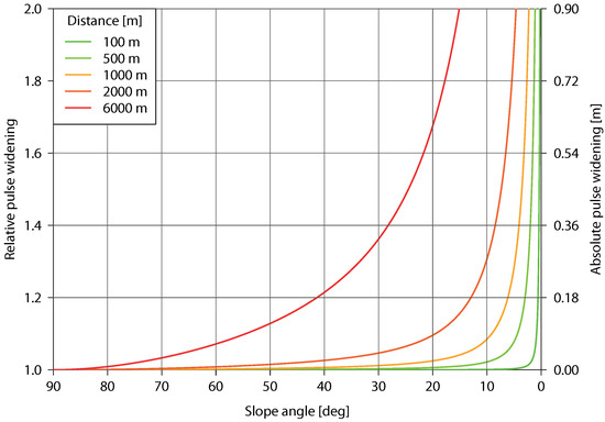
Figure 3.
The relationship of pulse widening (relative and absolute) and incidence angle of the laser beam at different scanning distances calculated after [51] and using the Riegl VZ®-6000 specific parameters = 0.12 mrad and = 3.
3.4. Point Cloud Registration
To facilitate the registration of the acquired point clouds, five square retro-reflective targets with known geometry (Figure 2b) were installed on stable ground around the active landslide part. In the far distance, three targets of m were installed while for the two targets located closer to the scanning positions, targets of m were chosen. The target’s directions were optimized for the selected scanning position on the opposite ridge (Figure 2b). The scanning position was determined by previous visibility analysis based on a digital terrain model (DTM) derived from airborne laser scanning (ALS). In addition, particular attention was paid to the safety of passers-by, preventing potential eye injuries due to the class 3B laser. However, the registration based on the retro-reflective targets’ centres did not provide acceptable results, mainly due to the large footprints in relation to the size of the targets at far distance. Furthermore, the limited number of targets distributed unevenly over the study area may have caused a minor tilting of the point clouds. Therefore, the ICP algorithm after [40] was applied to enhance the registration of the point clouds. However, a major challenge at quantifying displacement in multi-temporal 3D point clouds is to differentiate between stable and unstable areas in advance. The latter must be omitted during registration [37,52]. Therefore, only areas around the active part of the landslide which did not show significant displacements in the DGNSS measurements were considered for deriving two sets of transformation parameters by (i) using the targets’centres and (ii) applying the ICP algorithm. Subsequently, the two sets of transformation parameters were applied to the whole point cloud including stable and unstable areas.
3.5. Extraction of Geomorphological Breaklines
Geomorphological breaklines are linear features along strongly curved, either convex or concave morphological items (e.g., block edges, ridges, scarps). Their adjacent areas are characterized by undulating morphology with unique and recognizable settings. Assuming that the shape of the breaklines does not change between the data acquisitions, they are well suited to reproduce point correspondences in the multi-temporal data. These correspondences can be used to compute 3D displacement vectors representing the landslide’s movement in the period between the data acquisitions. To extract such areas, geometric point cloud features (e.g., geometric curvature) can be exploited, which are derived for each point considering a defined neighbourhood. The geometric curvature is based on locally derived eigenvectors representing the principle components in a covariance matrix. Eigenvectors and eigenvalues have proven feasible in many geometry-based classification approaches [53,54]. Furthermore, eigenvectors can be used to describe the geometry of different objects. Planar surfaces for example are characterized by two long eigenvectors parallel to the surface and one small eigenvector representing the surface normal (Figure 4a).
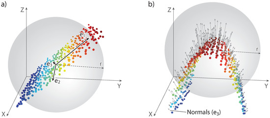
Figure 4.
Sketches of eigenvectors in a point cloud (a) representing a planar surface and (b) estimation of the geometric curvature within a spherical neighbourhood of radius r. The eigenvector with the lowest eigenvalue is used as surface normal (). A high deviation of the direction of the surface normals yields a high geometric curvature.
The geometric curvature can be expressed based on the surface normals within a defined neighbourhood, in which the normal vector is represented by the eigenvector with the smallest eigenvalue (Figure 4b) [55]. Following [55], the geometric curvature for each point p is based on the average difference between the direction of the local normal vector and the direction of the normal vectors of k considered neighbouring points j:
By defining an appropriate geometric curvature threshold, points representing highly convex and concave structures can be extracted and used for multi-temporal analyses. Parameters for eigenvector respectively normal vector estimation as well as the curvature threshold were tested to find an optimal conformity of the derived displacement vectors with the available DGNSS-measurements. Nine DGNSS survey points were suited, due to their spatially and chronologically overlap with the LRTLS point clouds. Search radius and minimum number of neighbours define the neighbourhood for the eigenvector calculation. Thus, besides the point density, the search radius and minimum number of neighbours influence the scale of point cloud represented morphologies. Consequently, the eigenvector based geometric curvature depends on these parameters. Considering a mean 2D point spacing of 5 cm and the size of the desired geomorphological features, the search radius for the eigenvector estimation was set to 50 cm and the minimum number of neighbours to 15 to exclude areas with a low point density from the calculation.
3.6. Point Neighbourhood Correspondence between Epochs
Originally, the ICP algorithm was developed by [40] for an efficient registration and improvement of already coarsely registered 3D shapes, including 3D point clouds. The proposed ICP-Matching algorithm implemented in the SAGA-LIS software [44] is based on the ICP algorithm after [40], but instead of enhancing the registration it is used to assess changes in the already registered multi-temporal point clouds which occurred between their acquisition. Figure 5a shows a workflow of the processing steps which are described in the following. First, both point clouds are segmented into uniform voxels of choosable size (Figure 5b). Then, the ICP algorithm is applied to each voxel, transforming the segmented point cloud of epoch two (slave) to the respective segment of epoch one (master) until either a selectable number of iterations or a distance threshold are reached. Furthermore, a maximum neighbourhood size can be specified, limiting the search radius for corresponding points of the extended ICP algorithm. Finally, point to surface correspondences [56] are computed, using the transformation matrix derived for each voxel to connect each point of the master point cloud with its corresponding surface in the slave point cloud (Figure 5c). Instead of deriving a set of transformation parameters for registration purposes, this extension of the ICP algorithm allows to derive local connections in multi-temporal point clouds, potentially representing changes which occurred between the acquisitions. In case of an active DSGSD the resulting connections can describe the movement which occurred between the point cloud acquisitions. In the present study voxels with an edge length of , a maximum neighbourhood size of , a limit of 10 iterations and a distance threshold of cm were used.
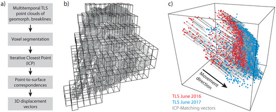
Figure 5.
Workflow (a) and principle of the ICP-Matching algorithm; (b) Voxels (here: 100 m edge length) dividing the point cloud into smaller chunks and (c) 3D displacement vectors of point-to-plane correspondences between point clouds of different epochs after applying the ICP-Matching algorithm.
3.7. Raster Neighbourhood Correspondence between Epochs
The aggregation of point clouds to raster formats using an adequate cell size and aggregation method enables a raster-based landslide displacement detection [17]. By recognizing corresponding raster value patterns in two images acquired at different points in time, translational surface displacement vectors can be calculated. This can be done by applying an image correlation approach (IMCORR), that was primarily developed to estimate horizontal flow velocity of glaciers [41,57].
A modified version of IMCORR was used in this study (IMCORR-DEM, [58]), considering imagery data and digital elevation models (DEMs) for the change detection. IMCORR-DEM allows to assess 2.5D displacements instead of a 2D displacement calculation implemented in the original version. Corresponding raster cells are matched based on spectral properties of shaded reliefs computed with the ambient occlusion method proposed by [59] based on the digital surface models (DSMs; 0.2 m spatial resolution) derived from the unclassified LRTLS point clouds. Complementary elevation data at the matched locations are then used to estimate the vertical displacement component, resulting in 2.5D displacement vectors. IMCORR-DEM is implemented in SAGA GIS and has proven feasible for assessing DSGSD-induced changes in a previous study [17]. Advantages and disadvantages of such a spectral and raster-based correspondence compared to geometry and point-based correspondence will be discussed in the following.
4. Results
4.1. Landslide Displacements Derived from DGNSS Measurements
Figure 6a shows the displacement direction and the annual horizontal landslide displacement measured with the help of a DGNSS. Because of the higher uncertainty of the measured elevation, the vertical displacement component is omitted. Observation points above the landslide’s crown do not show significant movement above the measurement accuracy. On the active part, significant annual displacements well above 50 cm and in some cases more than 100 cm in NW-SE direction are evident. Details about uncertainties at selected observation points are provided in Figure 6 and Table 1.
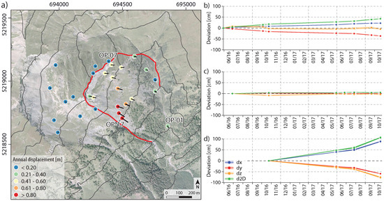
Figure 6.
Results of the DGNSS measurements. (a) Map showing approximate boundary (red line) of the active landslide part and the annual horizontal landslide displacement assessed with periodical DGNSS measurements at selected observation points. Examples of DGNSS time series for observation points OP-01 (b); OP-07 (c) and OP-17 (d) divided into their direction components and the related uncertainties (95% quantile). The length of the direction vectors, showing the displacement magnitude is 50-fold exaggerated. In case of OP-17 (d) two marking nails were installed. Their measurements are well in agreement. the map is shown in the UTM 32N projection (EPSG-Code: 25832).

Table 1.
Annual 2D and 3D displacements considering measurement uncertainty and variation (95% quantiles for the DGNSS measurements split in spatial components dX, dY and dZ and 1 standard deviation (SD) for the LRTLS measurements) derived from periodical DGNSS and LRTLS measurements at the respective observation points. All numbers are provided in centimetres.
4.2. Elevation Differences and Uncertainty of Multi-Temporal LRTLS Acquisitions
The comparison of digital terrain models (DTMs) derived from the classified TLS data acquired in June 2016 and 2017 can be used to determine elevation changes that have occurred within the active landslide part but also to quantify the registration accuracy by looking at assumed stable parts within the study area. A randomly distributed pattern of elevation gain and loss below the magnitude of the registration accuracy indicates a proper quality of the registration. Considering the resulting elevation differences of the approximated terrain (Figure 7a), the active part of the landslide below the scarp is characterized by a decrease of elevation while the lower part shows an increase. Vertical changes within one year of up to cm are clearly detectable and well above the measurement uncertainty. Along the movement direction, displacements in the order of 80 cm can be detected by comparing the representation of geomorphological features travelling on top of the landslide. No significant change can be detected around the active landslide part, excluding some elevation changes caused by still present avalanche snow or smaller debris flows or rock falls.
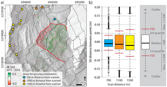
Figure 7.
Expected accuracy of the LRTLS measurements. (a) Map showing approximate boundary (red line) of the active landslide part and rasterized elevation changes (spatial resolution of 1 m) between the DTMs of the two TLS acquisitions. Changes below 0.1 m are not shown; (b) Boxplots showing point-to-plane distances (along the locally computed normal vector) between point clouds within selected stable areas in 700, 1100 and 1500 m distance from the scan position. IQR: Interquartile range, SD: standard deviation. The map is shown in the UTM 32N projection (EPSG-Code: 25832).
In addition, a point-cloud-based approach was applied to extend the information about the registration accuracy to the third dimension. Point cloud distance estimations were computed along normal vectors of locally fitted planes on assumed stable parts of the dataset. Selected stable areas scattered within various distances around the scan position (areas mapped in Figure 7a) including surfaces with aspects varying from to and slopes varying from to show a maximum 3D deviation of about cm (1 standard deviation) (Figure 7b). It is therefore expected that landslide displacements of at least 20 cm can be detected in the multi-temporal LRTLS data.
4.3. ICP-Matching Displacement Vectors
Applying a minimum curvature threshold of 0.2 reduces the point cloud covering the active area acquired in June 2016 from 100.0 M to 33.6 M points (34%) and the point cloud acquired in June 2017 from 204.8 M to 61.0 M points (30%). In total 33.4 M vectors were derived with the ICP-Matching algorithm within the extracted strongly curved active parts of the landslide. Figure 8a shows a map displaying the derived 3D displacement vectors, aggregated to median vectors per 2 m cell, represented by horizontal lines and coloured by 3D vector length. A distinct spatial pattern of displacement vectors describing the landslide movement within one year is observable. Below the crown at elevations above 2100 m displacements in the order of 0.6 to 0.8 m are dominating. In contrast, the north-eastern part below the crown is characterized by displacements less than 0.6 m. A maximum displacement with magnitudes exceeding 1.0 m can be observed at altitudes between 2000 and 2100 m. Further down the displacement declines to values below 0.8 m. Considering a detection limit of about 0.2 m, the currently active part of the landslide can be distinguished well from the surrounding stable areas.
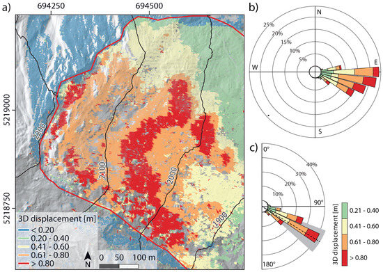
Figure 8.
Landslide displacement direction and magnitude derived from the ICP-Matching algorithm. (a) Map showing approximate boundary (red line) of the active landslide part and spatially aggregated 3D displacement vectors (one median value per 2 m cell); (b) Windrose showing the frequency of horizontal direction of movement and (c) windrose showing the frequency of the vertical direction of movement (0 would indicate a pure vertical movement upwards, 90 would represent a horizontal movement and 180 a pure vertical movement downwards). In (b,c) only displacement vectors with magnitudes above are shown. The dashed black line and the gray range in (c) indicate the mean and the standard deviation of the slope angle derived from the DTM. The map is shown in the UTM 32N projection (EPSG-Code: 25832).
The noticeable turn of movement from an east to a more south-east direction with decreasing altitude is confirmed by the distribution of the horizontal direction of the derived vectors (Figure 8a,b). Figure 8b shows the frequency distribution of vectors’ directions, classified by their magnitude. Displacement vectors in the upper part of the landslide are mainly directed eastwards. Further below, their magnitudes generally increase while their directions gradually change to south-east. The vertical components of the 3D displacement vectors show a mean of 27.4° indicating a lower inclination compared to the mean slope angle of 31.4° (Figure 8c).
4.4. Comparison of LRTLS- and DGNSS-Derived Displacements
Figure 9 shows the classified displacement vectors measured at the observation points with a DGNSS and derived area-wide with the ICP-Matching algorithm. Generally, the results are in agreement. Particularly in the areas considered stable, the results of the ICP-Matching algorithm are confirmed by the DGNSS measurements. Discrepancies between the results may be attributable to the considered dimensions (DGNSS: 2D, ICP-Matching: 3D).
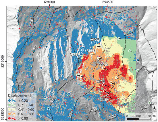
Figure 9.
Map showing classified displacement vectors derived from DGNSS measurements (circles) and from the ICP-Matching algorithm based on the two LRTLS point clouds (vectors). The results are in good agreement and exhibit comparable spatial patterns of landslide displacements. In case of the DGNSS results, horizontal displacements (2D) are shown. DGNSS vectors are 50-fold exaggerated. The map is shown in the UTM 32N projection (EPSG-Code: 25832).
The results of both techniques are directly compared at six DGNSS observation points (Figure 10). The DGNSS observation points OP07 and OP09, located on the crown of the landslide on stable grounds (mapped in Figure 9), do not show significant displacement considering the estimated measurement uncertainty (Figure 10a). The respective directions of the displacement vectors are therefore considered randomly distributed (Figure 10b). The survey points OP17, OP19, OP20 and OP23, distributed across the active part of the landslide (Figure 9), show easterly horizontal directions () in the upper part and more south-easterly directions () in the lower part of the landslide (Figure 10b). Horizontal directions either determined with DGNSS or based on the LRTLS indicate similar movement directions. Minor differences are apparent comparing the displacement magnitudes derived from LRTLS and DGNSS. The median of the point cloud derived vectors at observation point 17 is about 12 cm lower than the DGNSS-derived horizontal displacement component. At the observation points 19, 20 and 23 the median of the horizontal displacement derived with the ICP-Matching algorithm is about 4–6 cm above the DGNSS-derived horizontal displacement component. However, the more precise DGNSS vectors with an uncertainty range of 1.3–2.2 cm (95% quantile, Table 1) are within the variation of the point cloud derived vectors and within the median-aligned uncertainty range of 18 cm (95% quantile) of the LRTLS data. More details about the comparison of DGNSS and LRTLS displacements, either in horizontal direction or in 3D are provided in Table 1.
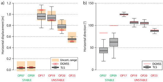
Figure 10.
Comparison of the (a) 2D displacement and (b) horizontal direction derived from periodical DGNSS measurements (red) and from the ICP-Matching algorithm based on the two LRTLS point clouds. Results are shown for six selected DGNSS observation points considering a 10 neighbourhood. Outliers are not shown.
4.5. IMCORR-DEM Displacement Vectors
In total 77,247 vectors covering the active part of the landslide were derived with the IMCORR-DEM algorithm, considering a 2 m spacing for the construction of correlating raster cells (Figure 11a). Data gaps are mainly related to the presence of high vegetation. In general, the spatial displacement pattern regarding the direction and magnitude of the derived vectors is similar to the results obtained with the ICP-Matching algorithm (Figure 8). However, distinct differences regarding the displacement magnitude in the upper active part of the landslide are obvious. There, displacements derived with the IMCORR-DEM algorithm are generally lower than those computed with the ICP-Matching algorithm. In contrast, displacements in the most active part between 2000 and 2100 m are in agreement.
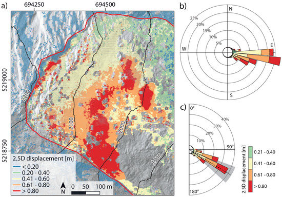
Figure 11.
Landslide displacement direction and magnitude derived from the IMCORR-DEM algorithm. (a) Map showing approximate boundary (red line) of the active landslide part and 2.5D displacement vectors; (b) Windrose showing the frequency of horizontal direction of movement and (c) windrose showing the frequency of the vertical direction of movement (0 would indicate a pure vertical movement upwards, 90 would represent a horizontal movement and 180 a pure vertical movement downwards). In (b,c) only displacement vectors with magnitudes above are shown. The dashed black line and the gray range in (c) indicate the mean and the standard deviation of the slope angle derived from the DTM. The map is shown in the UTM 32N projection (EPSG-Code: 25832).
Also the displacement vectors derived with the IMCORR-DEM algorithm show the gradual change of the landslide’s movement direction (Figure 11a,b). Below the crown the displacement vectors are mainly directed eastwards. Further below, they are increasingly directed south-east while their magnitudes generally increase. With a mean of 26.4°, the vertical components of the 2.5D displacement vectors fall below the respective mean of the results of the ICP-Matching algorithm (27.4°) and indicate a lower inclination compared to the mean slope angle of 31.4° (Figure 11c) as well.
4.6. Comparison of IMCORR-DEM and ICP-Matching Displacement Vectors
Comparing the resulting vector components of the raster-based (IMCORR-DEM) and point-based (ICP-Matching), distinct differences of the estimated 2.5D/3D displacement in the order of 10 cm can be observed (Figure 12b). The point-based method generally generates longer vectors than the raster-based approach. However, the horizontal and vertical vector components cover the same value range with an equal value distribution independent of the applied method (Figure 12c,d). Therefore, the applied method to derive displacement vectors either raster-based or point-based affects the postulated displacement magnitude but not the direction.
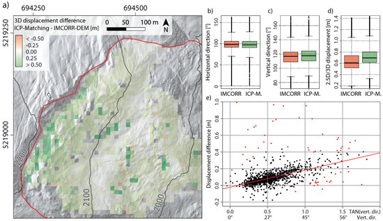
Figure 12.
Comparison of the resulting displacements derived from the applied algorithms. (a) Map showing approximate boundary (red line) of the active landslide part and differences of median 2.5D/3D displacement vectors (aggregated to a 10 m rasters) based on the ICP-Matching and the IMCORR-DEM algorithms. The boxplots show comparisons of the derived (b) horizontal direction; (c) vertical direction and (d) displacement magnitude; (e) Scatter plot with linear regression of the ICP-Matching generated tangent of vertical direction of movement and the difference (ICP-Matching—IMCORR-DEM) of estimated displacement. The red points were identified as outliers using the twofold mean of the Cook’s distance. These points were not used to build the regression. The map is shown in the UTM 32N projection (EPSG-Code: 25832).
Figure 12a shows the spatial distribution of displacement differences. Areas below the scarp, where vertical landslide movements are more dominant than horizontal movements (vertical direction up to 160) show major deviations of up to 50 cm between the resulting displacement magnitudes. There, the ICP-Matching approach generally provides longer displacements than the IMCORR- DEM approach. At the central parts of the landslide where horizontal movements are dominant (vertical direction less than 110 ) the estimated displacements either based on the ICP-Matching or the IMCORR-DEM algorithm do not show distinct differences. Consequently, a correlation between vertical movement direction and the difference of the estimated displacement between the ICP-Matching and IMCORR-DEM approach can be established (Figure 12e).
5. Discussion
The results of the applied methods, either point-based (ICP-Matching) or raster-based (IMCORR-DEM), show similarities but also differences when certain parameters like vector direction (vertical or horizontal) and magnitude are compared. The ICP-Matching approach provides one vector for each point-to-plane correspondence. The IMCORR-DEM approach on the other hand is not limited to the number of points but on the given spatial resolution of the derived raster data. This can be seen as the main factor controlling the resulting number of vectors. In this study the number of ICP-Matching vectors exceed the number of IMCORR-DEM vectors by a factor of over 400. Although the number of vectors is not directly interpretable as an indicator for the quality of the described displacement pattern, the advantage of the ICP-Matching approach is that displacement information can be acquired within areas where the IMCORR-DEM approach is not operable. Such areas are commonly steep walls or overhanging cliffs.
The comparison of ICP-Matching and IMCORR-DEM displacement vectors showed that deviations of vector magnitude are observable where sub-vertical landslide movements occur (Figure 12d,e). The original IMCORR approach was developed to quantify horizontal changes. However, the modified IMCORR-DEM approach additionally picks the elevation values of the starting and corresponding raster cells from the respective DEMs. The observed deviation of vector magnitude might therefore be caused by uncertainties related to the spatial resolution and the aggregation method used for computing the DEMs.
A coarse pre-alignment of multi-temporal point clouds is an essential requirement to apply the ICP algorithm for registration purposes. An ICP-based registration is therefore only feasible if coherent surfaces can be found within a limited neighbourhood. Exceeding this neighbourhood may result in erroneous correspondences which would not enhance the registration. Likewise, applying the ICP-Matching algorithm to assess landslide displacements implies limitations regarding their magnitude. In this study, this is accounted for by defining a voxel box size, determining a 3D neighbourhood for which the optimal translational and rotational parameters are estimated (Figure 5a). In addition, a suitable maximum search distance has to be chosen, allowing the ICP-Matching algorithm to converge properly. Both parameters must be chosen with respect to the expected maximum landslide displacement as well as the point density of the available data.
Furthermore, the presented ICP-Matching algorithm is only suitable if predominantly translational displacement has occurred. In case the geometry of geomorphological features has changed between the observed epochs adequate point-to-plane correspondences can not be reproduced accurately.
The results of the IMCORR-DEM approach showed that it is feasible to generate vectors at less curved areas, where correspondences of raster patterns can be established while point-to-plane correspondences are not feasible. Another advantage of the IMCORR-DEM approach is that corresponding raster patterns can also be identified if they have travelled over longer distances. Therefore faster moving processes are detectable by using the IMCORR-DEM approach but probably not by using the ICP-Matching approach. A point-cloud-based detection of corresponding far travelled features might be feasible by defining distinct objects which can be recognized in every epoch.
6. Conclusions
In the present study multi-temporal long-range terrestrial laser scanning is applied to assess area-wide 3D movement patterns of a DSGSD in the Schmirn valley (Tyrol, Austria). 3D displacements with a mean magnitude of 0.62 m per year derived from point clouds acquired with a Riegl VZ®-6000 long-range laser scanner in 2016 and 2017 are clearly above the measurement uncertainty of cm. Displaced geomorphological breaklines (e.g., block edges, terrain ridges, scarps) can be automatically extracted from the point clouds by using locally computed eigenvectors and -values. A workflow based on the well-known ICP approach is proposed to derive 3D displacement vectors for the extracted geomorphological features. These LRTLS derived vectors are in good agreement with the additionally acquired reference data at selected observation points using a DGNSS. Maximum differences between LRTLS and DGNSS-derived vectors of 12 cm are observable whereas minor differences of 4–6 cm are more frequent. Benefits of the presented ICP-Matching algorithm are highlighted by comparing the results with those of a modified state of the art raster-based approach (IMCORR-DEM).
The presented ICP-Matching algorithm is designed to process multi-temporal 3D point clouds, which can describe complex surfaces in great detail. Raster-based approaches process aggregated 2D or 2.5D raster data which consequently include less topographic details. Therefore, the ICP-Matching algorithm can outperform raster-based approaches particularly in complex Alpine terrain. However, on smooth terrain only the applied raster-based IMCORR-DEM approach could provide results. Therefore, in order to derive area-wide maps of landslide displacement, the results of both methods could be integrated.
In order to generally enhance the detection threshold of landslide displacement future research involving LRTLS should deepen the understanding of the influence of environmental conditions on the measurements. The effects of atmospheric conditions are rarely considered in such studies. Also the interaction of LRTLS and low vegetation is rarely addressed. These improvements are required to enhance the accuracy of LRTLS and to enable also the monitoring of slower moving landslides.
Author Contributions
J.P., T.Z. and M.R. conceived and designed the experiments; J.P. and T.Z. acquired and analyzed the data; M.B. and V.W. contributed analysis tools and helped interpreting the results; J.P. and T.Z. wrote the paper.
Funding
This research was funded by Euregio Science Fund: IPN 18-N30.
Acknowledgments
We thank Jakob Balassa and Andreas Mayr for their assistance in the field. This research is conducted within the project LEMONADE (http://lemonade.mountainresearch.at).
Conflicts of Interest
The authors declare no conflict of interest.
References
- Gili, J.A.; Corominas, J.; Rius, J. Using Global Positioning System techniques in landslide monitoring. Eng. Geol. 2000, 55, 167–192. [Google Scholar] [CrossRef]
- Squarzoni, C.; Delacourt, C.; Allemand, P. Differential single-frequency GPS monitoring of the La Valette landslide (French Alps). Eng. Geol. 2005, 79, 215–229. [Google Scholar] [CrossRef]
- Hofmann, R.; Sausgruber, J.T. Creep behaviour and remediation concept for a deep-seated landslide, Navistal, Tyrol, Austria. Geomechan. Tunn. 2017, 10, 59–73. [Google Scholar] [CrossRef]
- Thuro, K.; Singer, J.; Festl, J.; Wunderlich, T.; Wasmeier, P.; Reith, C.; Heunecke, O.; Glabsch, J.; Schuhbäck, S. New landslide monitoring techniques—developments and experiences of the alpEWAS project. J. Appl. Geodesy 2010, 4, 69–90. [Google Scholar] [CrossRef]
- Angeli, M.G.; Pasuto, A.; Silvano, S. A critical review of landslide monitoring experiences. Eng. Geol. 2000, 55, 133–147. [Google Scholar] [CrossRef]
- Mikoš, M.; Brilly, M.; Fazarinc, R.; Ribičič, M. Strug landslide in W Slovenia: A complex multi-process phenomenon. Eng. Geol. 2006, 83, 22–35. [Google Scholar] [CrossRef]
- Gance, J.; Malet, J.P.; Supper, R.; Sailhac, P.; Ottowitz, D.; Jochum, B. Permanent electrical resistivity measurements for monitoring water circulation in clayey landslides. J. Appl. Geophys. 2016, 126, 98–115. [Google Scholar] [CrossRef]
- Wilkinson, P.B.; Chambers, J.E.; Meldrum, P.I.; Gunn, D.A.; Ogilvy, R.D.; Kuras, O. Predicting the movements of permanently installed electrodes on an active landslide using time-lapse geoelectrical resistivity data only. Geophys. J. Int. 2010, 183, 543–556. [Google Scholar] [CrossRef]
- Petley, D.; Mantovani, F.; Bulmer, M.; Zannoni, A. The use of surface monitoring data for the interpretation of landslide movement patterns. Geomorphology 2005, 66, 133–147. [Google Scholar] [CrossRef]
- Simeoni, L.; Mongiovì, L. Inclinometer Monitoring of the Castelrotto Landslide in Italy. J. Geotech. Geoenviron. Eng. 2007, 133, 653–666. [Google Scholar] [CrossRef]
- Lavender, S.; Lavender, A. Practical Handbook of Remote Sensing; CRC Press: Boca Raton, FL, USA, 2015. [Google Scholar]
- Wasowski, J.; Bovenga, F. Investigating landslides and unstable slopes with satellite Multi Temporal Interferometry: Current issues and future perspectives. Eng. Geol. 2014, 174, 103–138. [Google Scholar] [CrossRef]
- Schlögel, R.; Thiebes, B.; Mulas, M.; Cuozzo, G.; Notarnicola, C.; Schneiderbauer, S.; Crespi, M.; Mazzoni, A.; Mair, V.; Corsini, A. Multi-Temporal X-Band Radar Interferometry Using Corner Reflectors: Application and Validation at the Corvara Landslide (Dolomites, Italy). Remote Sens. 2017, 9, 739. [Google Scholar] [CrossRef]
- Tarchi, D.; Casagli, N.; Moretti, S.; Leva, D.; Sieber, A.J. Monitoring landslide displacements by using ground-based synthetic aperture radar interferometry: Application to the Ruinon landslide in the Italian Alps. J. Geophys. Res. Solid Earth 2003, 108. [Google Scholar] [CrossRef]
- Bardi, F.; Frodella, W.; Ciampalini, A.; Bianchini, S.; Del Ventisette, C.; Gigli, G.; Fanti, R.; Moretti, S.; Basile, G.; Casagli, N. Integration between ground based and satellite SAR data in landslide mapping: The San Fratello case study. Geomorphology 2014, 223, 45–60. [Google Scholar] [CrossRef]
- Barbarella, M.; Fiani, M.; Lugli, A. Landslide monitoring using multitemporal terrestrial laser scanning for ground displacement analysis. Geomat. Nat. Hazards Risk 2015, 6, 398–418. [Google Scholar] [CrossRef]
- Fey, C.; Rutzinger, M.; Wichmann, V.; Prager, C.; Bremer, M.; Zangerl, C. Deriving 3D displacement vectors from multi-temporal airborne laser scanning data for landslide activity analyses. GISci. Remote Sens. 2015, 52, 437–461. [Google Scholar] [CrossRef]
- Corsini, A.; Castagnetti, C.; Bertacchini, E.; Rivola, R.; Ronchetti, F.; Capra, A. Integrating airborne and multi-temporal long-range terrestrial laser scanning with total station measurements for mapping and monitoring a compound slow moving rock slide. Earth Surf. Process. Landf. 2013, 38, 1330–1338. [Google Scholar] [CrossRef]
- Razak, K.; Straatsma, M.; van Westen, C.; Malet, J.P.; de Jong, S. Airborne laser scanning of forested landslides characterization: Terrain model quality and visualization. Geomorphology 2011, 126, 186–200. [Google Scholar] [CrossRef]
- Balek, J.; Blahut, J. A critical evaluation of the use of an inexpensive camera mounted on a recreational unmanned aerial vehicle as a tool for landslide research. Landslides 2017, 14, 1217–1224. [Google Scholar] [CrossRef]
- Stumpf, A.; Malet, J.P.; Allemand, P.; Pierrot-Deseilligny, M.; Skupinski, G. Ground-based multi-view photogrammetry for the monitoring of landslide deformation and erosion. Geomorphology 2015, 231, 130–145. [Google Scholar] [CrossRef]
- Hanssen, R.F. Radar Interferometry: Data Interpretation and Error Analysis; Springer Science & Business Media: Berlin, Germany, 2001; Volume 2. [Google Scholar]
- Fiorucci, F.; Giordan, D.; Santangelo, M.; Dutto, F.; Rossi, M.; Guzzetti, F. Criteria for the optimal selection of remote sensing optical images to map event landslides. Nat. Hazards Earth Syst. Sci. 2018, 18, 405–417. [Google Scholar] [CrossRef]
- Harpold, A.A.; Marshall, J.A.; Lyon, S.W.; Barnhart, T.B.; Fisher, B.A.; Donovan, M.; Brubaker, K.M.; Crosby, C.J.; Glenn, N.F.; Glennie, C.L.; et al. Laser vision: Lidar as a transformative tool to advance critical zone science. Hydrol. Earth Syst. Sci. 2015, 19, 2881–2897. [Google Scholar] [CrossRef]
- Fey, C.; Wichmann, V. Long-range terrestrial laser scanning for geomorphological change detection in alpine terrain—handling uncertainties. Earth Surf. Process. Landf. 2017, 42, 789–802. [Google Scholar] [CrossRef]
- Bremer, M.; Rutzinger, M.; Wichmann, V. Derivation of tree skeletons and error assessment using LiDAR point cloud data of varying quality. ISPRS J. Photogramm. Remote Sens. 2013, 80, 39–50. [Google Scholar] [CrossRef]
- James, M.R.; Pinkerton, H.; Applegarth, L.J. Detecting the development of active lava flow fields with a very-long-range terrestrial laser scanner and thermal imagery. Geophys. Res. Lett. 2009, 36, L22305. [Google Scholar] [CrossRef]
- Travelletti, J.; Oppikofer, T.; Delacourt, C.; Malet, J.; Jaboyedoff, M. Monitoring landslide displacements during a controlled rain experiment using a long-range terrestrial laser scanning (TLS). Int. Arch. Photogramm. Remote Sens. Spat. Inf. Sci. 2008, 37, 485–490. [Google Scholar]
- Fischer, M.; Huss, M.; Kummert, M.; Hoelzle, M. Application and validation of long-range terrestrial laser scanning to monitor the mass balance of very small glaciers in the Swiss Alps. Cryosphere 2016, 10, 1279–1295. [Google Scholar] [CrossRef]
- Gabbud, C.; Micheletti, N.; Lane, S.N. Lidar measurement of surface melt for a temperate Alpine glacier at the seasonal and hourly scales. J. Glaciol. 2015, 61, 963–974. [Google Scholar] [CrossRef]
- Mukupa, W.; Roberts, G.W.; Hancock, C.M.; Al-Manasir, K. A review of the use of terrestrial laser scanning application for change detection and deformation monitoring of structures. Survey Rev. 2017, 49, 99–116. [Google Scholar] [CrossRef]
- Telling, J.; Lyda, A.; Hartzell, P.; Glennie, C. Review of earth science research using terrestrial laser scanning. Earth-Sci. Rev. 2017, 169, 35–68. [Google Scholar] [CrossRef]
- Monserrat, O.; Crosetto, M. Deformation measurement using terrestrial laser scanning data and least squares 3D surface matching. ISPRS J. Photogramm. Remote Sens. 2008, 63, 142–154. [Google Scholar] [CrossRef]
- Prokop, A.; Panholzer, H. Assessing the capability of terrestrial laser scanning for monitoring slow moving landslides. Nat. Hazards Earth Syst. Sci. 2009, 9, 1921–1928. [Google Scholar] [CrossRef]
- Chen, X.; Yu, K.; Wu, H. Determination of Minimum Detectable Deformation of Terrestrial Laser Scanning Based on Error Entropy Model. IEEE Trans. Geosci. Remote Sens. 2018, 56, 105–116. [Google Scholar] [CrossRef]
- Kromer, R.A.; Abellán, A.; Hutchinson, D.J.; Lato, M.; Chanut, M.A.; Dubois, L.; Jaboyedoff, M. Automated terrestrial laser scanning with near-real-time change detection–monitoring of the Séchilienne landslide. Earth Surf. Dyn. 2017, 5, 293–310. [Google Scholar] [CrossRef]
- Wujanz, D.; Krueger, D.; Neitzel, F. Identification of stable areas in unreferenced laser scans for deformation measurement. Photogramm. Rec. 2016, 31, 261–280. [Google Scholar] [CrossRef]
- Ghuffar, S.; Székely, B.; Roncat, A.; Pfeifer, N. Landslide displacement monitoring using 3D range flow on airborne and terrestrial LiDAR data. Remote Sens. 2013, 5, 2720–2745. [Google Scholar] [CrossRef]
- Mayr, A.; Rutzinger, M.; Bremer, M.; Oude Elberink, S.; Stumpf, F.; Geitner, C. Object-based classification of terrestrial laser scanning point clouds for landslide monitoring. Photogramm. Rec. 2017, 32, 377–397. [Google Scholar] [CrossRef]
- Besl, P.J.; McKay, N.D. A method for registration of 3-D shapes. IEEE Trans. Pattern Anal. Mach. Intell. 1992, 14, 239–256. [Google Scholar] [CrossRef]
- Fahnestock, M.A.; Scambos, T.A.; Bindschadler, R.A. Semi-Automated Ice Velocity Determination from Satellite Imagery. Eos Trans. AGU 1992, 73, 493. [Google Scholar]
- Rockenschaub, M.; Kolenprat, B.; Nowotny, A. Das westliche Tauernfenster. In Arbeitstagung 2003: Blatt 148 Brenner; Geologische Bundesanstalt: Wien, Austria, 2003. [Google Scholar]
- Riegl. Operating and Processing Software RiScan Pro; Riegl: Horn, Austria, 2016. [Google Scholar]
- Wichmann, V. Laserdata LIS Command Reference, Version 3.0; Laserdata: Innsbruck, Austria, 2015. [Google Scholar]
- Axelsson, P. DEM generation from laser scanner data using adaptive TIN models. Int. Arch. Photogramm. Remote Sens. 2000, 33, 110–117. [Google Scholar]
- Prokop, A. Assessing the applicability of terrestrial laser scanning for spatial snow depth measurements. Cold Reg. Sci. Technol. 2008, 54, 155–163. [Google Scholar] [CrossRef]
- Beraldin, J.A.; Blais, F.; Lohr, U. Airborne and Terrestrial Laser Scanning; Whittles Publishing: Dunbeath, UK, 2010; Chapter Laser Scanning Technology; pp. 1–41. [Google Scholar]
- Riegl Laser Measurement Systems GmbH. 3D Terrestrial Laser Scanner Riegl VZ-4000 I Riegl VZ-6000 General Description and Data Interfaces; Riegl Laser Measurement Systems GmbH: Horn, Austria, 2013. [Google Scholar]
- Lichti, D.D.; Gordon, S.J. Error propagation in directly georeferenced terrestrial laser scanner point clouds for cultural heritage recording. In Proceedings of the FIG Working Week, Athens, Greece, 22–27 May 2004; pp. 22–27. [Google Scholar]
- Schaer, P.; Skaloud, J.; Landtwing, S.; Legat, K. Accuracy estimation for laser point cloud including scanning geometry. Int. Arch. Photogramm. Remote Sens. Spat. Inf. Sci. 2007, 37, 851–856. [Google Scholar]
- Pfennigbauer, M.; Wolf, C.; Ullrich, A. Enhancing online waveform processing by adding new point attributes. In Proceedings of the Laser Radar Technology and Applications XVIII, Baltimore, MD, USA, 6–7 May 2014; Turner, M.D., Kamerman, G.W., Eds.; International Society for Optics and Photonics: Bellingham, WA, USA, 2013; Volume 8731, p. 873104. [Google Scholar] [CrossRef]
- Wujanz, D.; Avian, M.; Krueger, D.; Neitzel, F. Identification of stable areas in unreferenced laser scans for automated geomorphometric monitoring. Earth Surf. Dyn. 2018, 6, 303–317. [Google Scholar] [CrossRef]
- Belton, D.; Lichti, D.D. Classification and segmentation of terrestrial laser scanner point clouds using local variance information. Int. Arch. Photogramm. Remote Sens. Spat. Inf. Sci. 2006, 36, 44–49. [Google Scholar]
- Pauly, M.; Gross, M.; Kobbelt, L.P. Efficient simplification of point-sampled surfaces. In Proceedings of the Conference on Visualization’02 IEEE Computer Society, Boston, MA, USA, 27 October–1 November 2002; pp. 163–170. [Google Scholar] [CrossRef]
- Bae, K.; Lichti, D. Automated Registration of Unorganised Point Clouds from Terrestrial Laser Scanners. In Proceedings of the XXth ISPRS Congress: Geo-Imagery Bridging Continents, Istanbul, Turkey, 12–23 July 2004; Altan, P.O., Ed.; 2004; pp. 1–6. [Google Scholar]
- Chen, Y.; Medioni, G. Object modelling by registration of multiple range images. Image Vis. Comput. 1992, 10, 145–155. [Google Scholar] [CrossRef]
- Scambos, T.A.; Dutkiewicz, J.C.; Wilson, J.; Bindschadler, R. Application of Image Cross-Correlation to the Measurement of Glacier Velocity Using Satellite Image Data. Remote Sens. Environ. 1992, 42, 177–186. [Google Scholar] [CrossRef]
- Bremer, M. IMCORR—Feature Tracking. SAGA Module Reference. 2012. Available online: http://www.saga-gis.org (accessed on 25 October 2018).
- Tarini, M.; Cignoni, P.; Montani, C. Ambient occlusion and edge cueing for enhancing real time molecular visualization. IEEE Trans. Vis. Comput. Gr. 2006, 12. [Google Scholar] [CrossRef] [PubMed]
© 2018 by the authors. Licensee MDPI, Basel, Switzerland. This article is an open access article distributed under the terms and conditions of the Creative Commons Attribution (CC BY) license (http://creativecommons.org/licenses/by/4.0/).