Analysis and Simulation on Imaging Performance of Backward and Forward Bistatic Synthetic Aperture Radar

Abstract

In recent years, bistatic synthetic aperture radar (SAR) technique has attracted considerable and increasing attention. Compared to monostatic SAR for which only the backscattering is measured, bistatic SAR expands the scattering measurements in aspects of angular region and polarization, and greatly enhances the capability of remote sensing over terrain and sea. It has been pointed out in recent theoretical researches that bistatic scattering measured in the forward region is preferable to that measured in the backward region in lines of surface parameters retrieval. In the forward region, both dynamic range and signal sensitivity increase to a great extent. For these reasons, bistatic SAR imaging is desirable. However, because of the separated positions of the transmitter and receiver, the degrees of freedom in the parameter space is increased and the forward bistatic imaging is more complicated than the backward bistatic SAR in the aspects of bistatic range history, Doppler parameter estimation and motion compensation, et, al. In this study, we analyze bistatic SAR in terms of ground range resolution, azimuth resolution, bistatic range history and signal to noise ratio (SNR) in different bistatic configurations. Effects of system motion parameters on bistatic SAR imaging are investigated through analytical modeling and numerical simulations. The results indicate that the range resolution is extremely degraded in some cases in forward bistatic SAR imaging. In addition, due to the different imaging projection rules between backward and forward bistatic SAR, the ghost point is produced in the forward imaging. To avoid the above problems, the forward bistatic imaging geometry must be carefully considered. For a given application requirement with the desired imaging performances, the design of the motion parameters can be considered as a question of solving the nonlinear equation system (NES). Then the improved chaos particle swarm optimization (CPSO) is introduced to solve the NES and obtain the optimal solutions. And the simulated imaging results are used to test and verify the effectiveness of CPSO. The results help to deepen understanding of the constraints and properties of bistatic SAR imaging and provide the reference to the optimal design of the motion parameters for a specific requirement, especially in forward bistatic configurations.

1. Introduction

Bistatic synthetic aperture radars (SAR) have attracted increasing attention in the SAR remote sensing area over the last decade [1,2]. Compared to monostatic SAR, bistatic SAR shows superiority in numerous earth observations because the transmitter and the receiver can be distributed at the desired angular position. It is evident that in the bistatic mode, the forward scattering coefficients are generally more sensitive to the target’s physical parameters than that of backscattering [3,4]. The theoretical researches [5,6] indicate that the forward scattering coefficients of a target in different directions usually provide more abundant and useful information than the traditional backward backscattering; also, for a target with a low RCS in the monostatic SAR, by bistatic SAR one can find a distinct dual-angle configuration to increase the RCS to make these targets visible in the final image. As the obtained scattering information becomes richer, bistatic SAR theoretically offers a better study on target scattering mechanisms and a greater ability for target classification and recognition [7]. Therefore, it is clear that a new forward scattering bistatic geometry is necessary to meet a large number of observational demands and it will be a great complementarity to the traditional monostatic observation. Although the existing bistatic system—TanDEM-X, has good application prospects in environmental and climate monitoring, it should still be considered as a quasi-monostatic configuration and as a result, the forward scattering information cannot be obtained yet in practical satellite mission.

Compared to monostatic SAR imaging, bistatic imaging can acquire the echo information of a target from different directions, avoid strong reflection points and improve the SNR. However, because of the two separated carrier platforms, the performance analysis of the bistatic SAR imaging is more complicated than that of monostatic SAR in terms of bistatic range history, two-dimensional resolution, Doppler parameter estimation, motion compensation and so on, especially in the forward mode. As the most important performance index, bistatic spatial resolution can be calculated by the following three methods: gradient method [8], generalized ambiguity function (GFA) [9] and the K-space method [10]. In reference [11], the spatial resolution of general hybrid bistatic SAR with mid-Earth orbit was analyzed and it notes the effects of the imaging configuration on imaging resolution. Yicheng Jiang et al. [12] deduced the resolution of the geosynchronous transmitter and UAV receiver (GEO-UAV BiSAR) on the basis of the gradient method and analyzed the configuration influences on the range and azimuth resolution. Zhichao Sun et al. [13] analyzed the spatial resolution characteristics of inclined geosynchronous spaceborne-airborne bistatic SAR based on the GFA method and solved a nonlinear equation system to guide the receiver motion parameters. In the abovementioned studies, the characteristics of spatial resolution in the whole scattering space have still not been given directly.

Keeping the characteristics of different configurations in view, the bistatic SAR imaging algorithm has been intensively studied. Due to the space-variance and topography-sensitivity of bistatic SAR, it is a challenge to build efficient image formation algorithms in the Fourier domain [14,15,16] in the bistatic SAR with a large bistatic angle but it can be processed effectively in the time-domain. However, the time-domain focusing algorithms ordinarily have huge computational costs, for example, the classical time-domain back-projection (BP) algorithm. Consequently, many efficient implementations of BP have been proposed [17,18,19,20,21]. However, most of these works focused on quasi-monostatic imaging geometries (in the backward scattering zone), or in non-formation geometry (spaceborne-airborne, et al.); few published works have addressed the forward bistatic imaging purposes with a large baseline and dual angular bistatic configuration in formation, which has been highly desired by remote sensing applications. In addition, the bistatic range history is closely related to the bistatic geometrics configuration and requires specific investigations.

This paper concerns imaging geometric properties and the related power considerations of the bistatic observation geometry based on the system parameters of Satellites for Observation and Communications-Companion Satellite (SAOCOM-CS) [22,23,24] in formation mode and focuses on the forward bistatic. The results offer a deeper understanding of the large baseline bistatic SAR imaging and help to design a reliable bistatic imaging system. In Section 2, we talk about the bistatic imaging geometry and signal model. Then, the imaging properties of bistatic SAR in terms of ground range resolution, Azimuth resolution, bistatic range history and signal to noise ratio (SNR) will be discussed. In addition, the BP algorithm for focusing is briefly reviewed. Section 3 analyses the imaging properties and power considerations with respect to receiver motion parameters. An improved CPSO is used to select the optimal motion parameters under the desired imaging performance requirements. In addition, some simulation results are shown to support the analysis. Section 4 concludes the paper with a preliminary summary and outlooks for further study.

2. Model and Methods in Analyzing Geometric Properties and Related Power Considerations

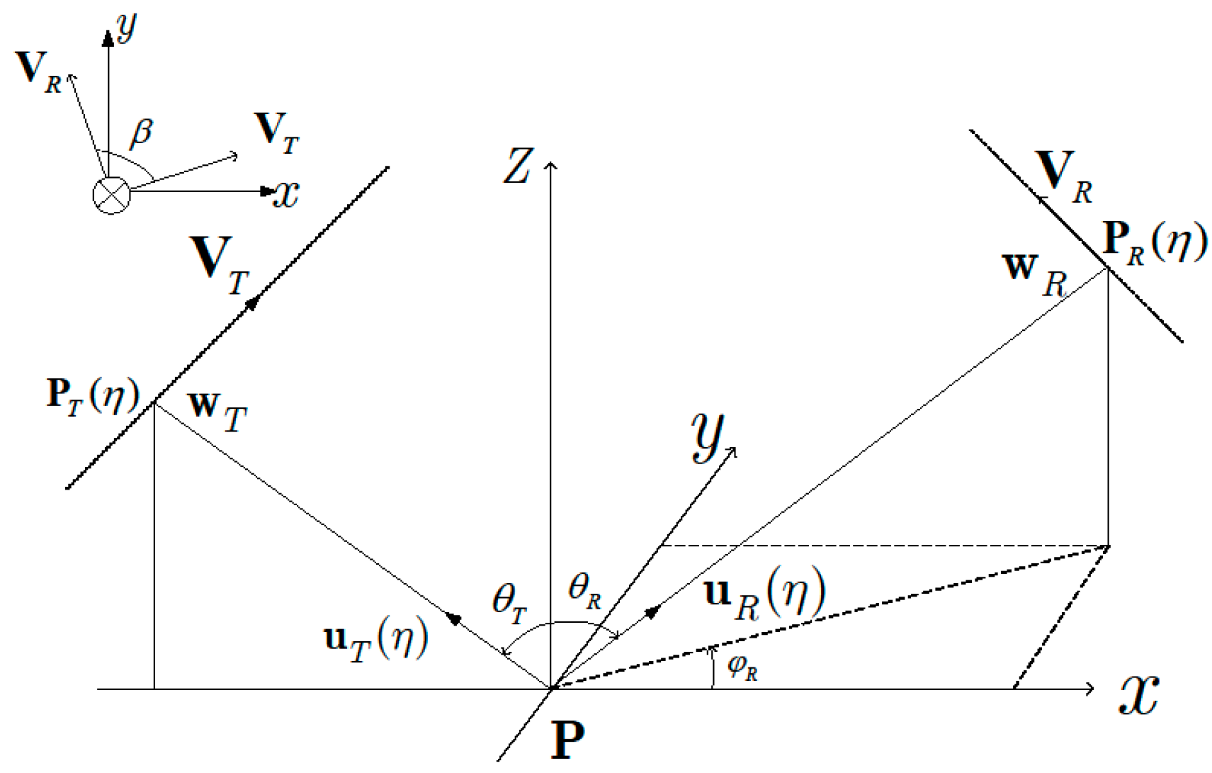
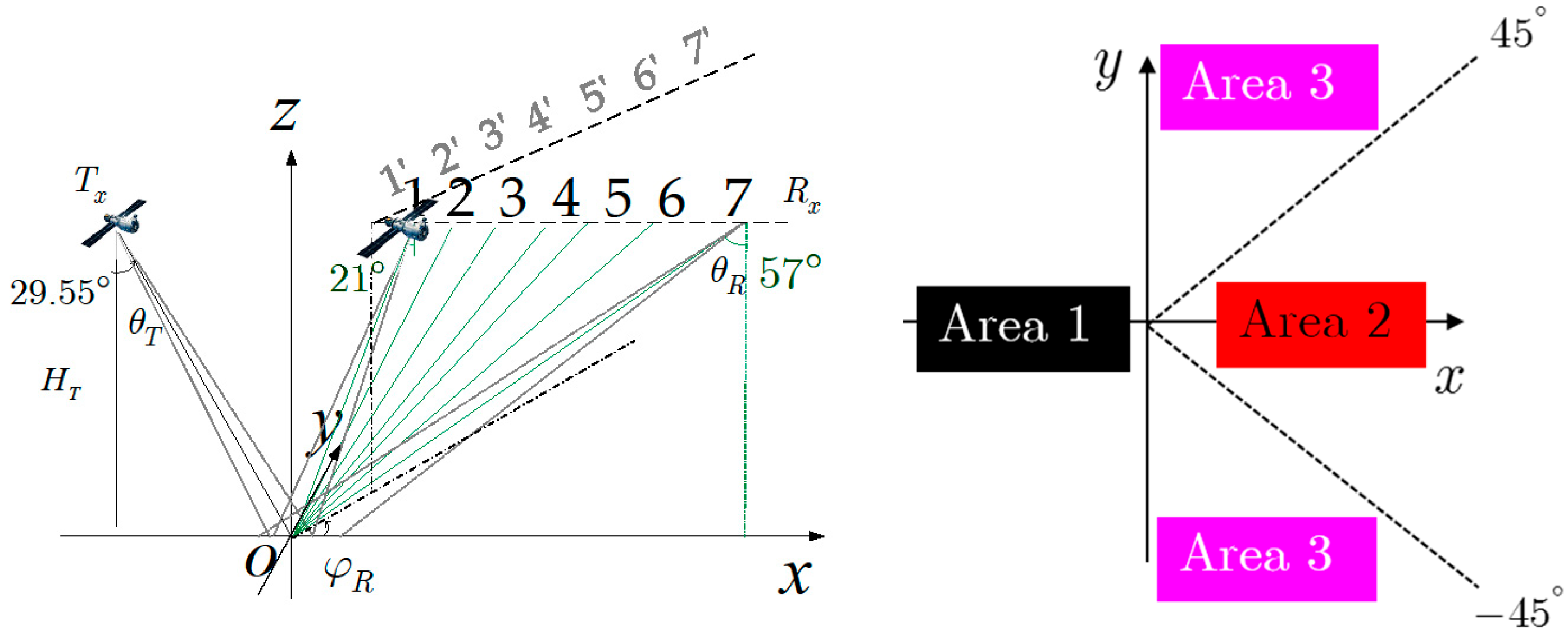
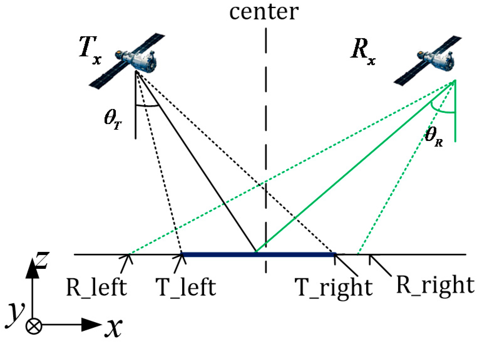
2.1. Imaging Geometry and Signal Model

In this chapter, the geometric property and power considerations of backward and forward bistatic SAR will be discussed based on the imaging geometry as depicted in Figure 1. In the imaging geometry, ${\theta }_T$ and ${\phi }_T$ are the incidence angle and transmitted azimuth angle and ${\theta }_R$ and ${\phi }_R$ the received incidence angle and received azimuth angle, with subscripts T and R denoting the transmitter and the receiver; the imaging space perhaps can be roughly divided into two zones, assuming a positive azimuth angle is counter-clockwise from the x-axis; the forward imaging zone is the area with the azimuth angle in the range of ${\phi }_R\in (0°,90°)\cup (270°,360°)$ and another part belongs to the backward imaging zone. $P_T(\eta )$ and $P_R(\eta )$ are the instantaneous position vectors; $V_T$ and $V_R$ are the velocity vectors; $u_T(\eta )$ and $u_R(\eta )$ are the unit vectors in the direction from target P to the transmitter and receiver, respectively, at $\eta$, with $w_T(\eta )$ and $w_R(\eta )$ denoting the angular velocities of the transmitter and receiver, respectively, at the time $\eta$; $\beta$ is the velocity angle between the transmitter and the receiver velocity vectors. Notice that the monostatic backward imaging and bistatic forward specular imaging are located at ${\theta }_T={\theta }_R,{\phi }_R=180°$ and ${\theta }_T={\theta }_R,{\phi }_R=0°$, respectively.

In the stripmap mode bistatic SAR, for analysis, some hypotheses are made in our study: first, we consider that the transmitter and the receiver sweep a continuous strip synchronously during the entire observation time and second, the stop-and-go model is adopted. Finally, the ground plane of the imaging scenario is flat. If the curvature of the earth is considered, the whole scene can be divided into sub blocks so that the following analysis is still valid. Suppose that the transmitter sends a pulsed signal with duration time $T_p$ and the carrier frequency $f_c$, defined as:

$$s(\tau )=w_r(\tau )\exp [j(2\pi f_c\tau +\pi K_r{\tau }^2)]$$

(1)

where $\tau$ is the range time, $K_r$ is the chirp rate and $w_r$ is a rectangular gate function with width $T_p$. The demodulated baseband signal from a point target having a constant scatter amplitude $A_0$ is of the form

$$s_r(\tau ,\eta ){=\mathrm{A}}_0{w}_r(\tau -\frac{2R_{bi}(\eta )}{c})w_a(\eta )\exp \left\{-j\frac{4\pi f_c{R}_{bi}(\eta )}{c})+j\pi K_r{(\tau -\frac{2R_{bi}(\eta )}{c})}^2\right\}$$

(2)

where $c$ denotes the speed of light, $\eta$ is the cross-range time, $w_a$ is the antenna pattern in the cross-range direction and $R_{bi}(\eta )$ is the bistatic range, which is the sum of the ranges from the transmitter and the receiver to the target.

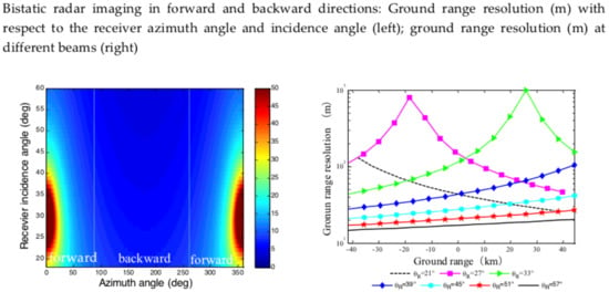
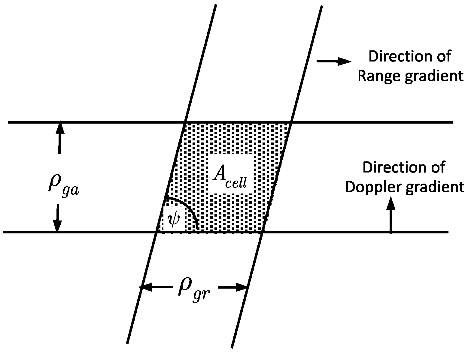
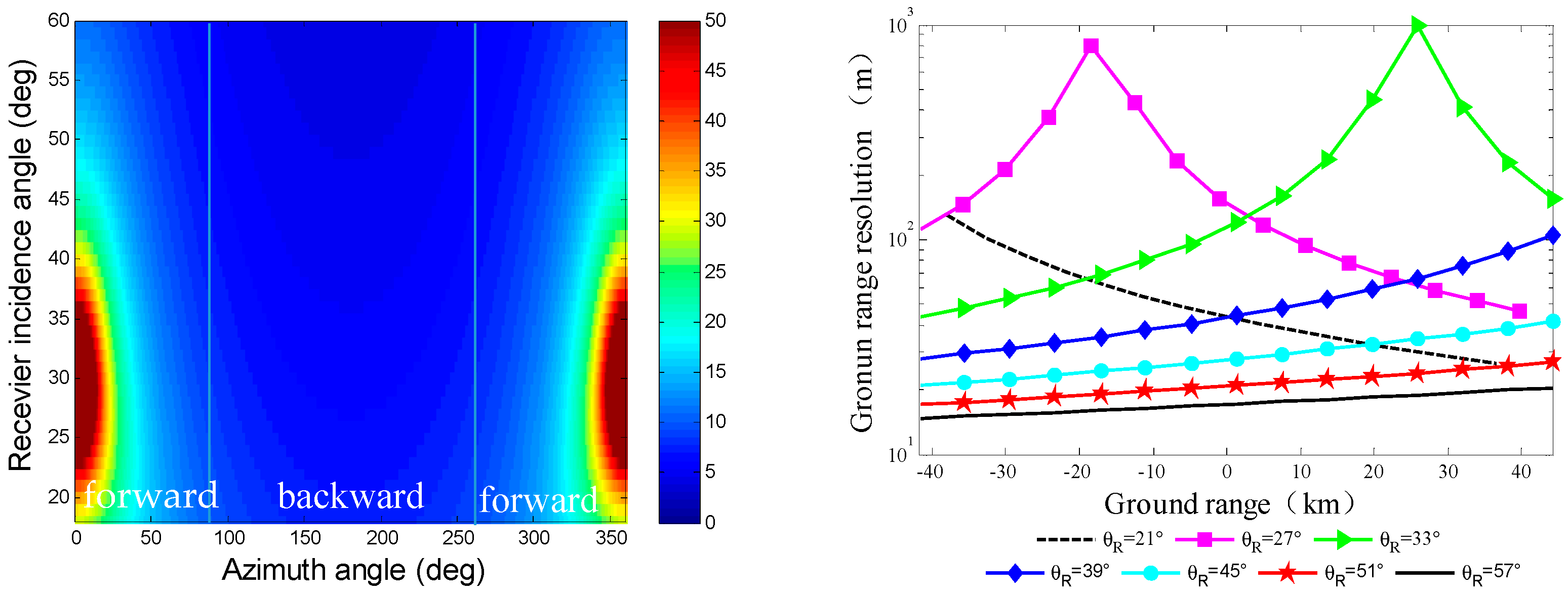
2.2. Range Resolution and Azimuth Resolution

We now consider the two-dimensional ground resolution in a general configuration of bistatic SAR as shown in Figure 1. For the targets with a constant arrival time satisfy an iso-range surface $t(\eta )=\frac{\Vert P_T(\eta )-P\Vert +\Vert P_R(\eta )-P\Vert }{c}$, upon projecting to the iso-range gradient vector, one can obtain the general form of the bistatic ground range resolution [8].

$${\rho }_{gr}=\frac{\kappa c}{B\Vert P_{Z_s}^{\perp }{u}_T\left(\eta \right)+P_{Z_s}^{\perp }{u}_R\left(\eta \right)\Vert }$$

(3)

where $\kappa =0.886$ when the antenna patterns and ranging waveform can be approximated by the rectangle pulse function; $B$ is the signal bandwidth; $P_{Z_s}^{\perp }$ is the ground projection matrix given by

$$P_{Z_s}^{\perp }=\left[\begin{array}{ccc}1& 0& 0\\ 0& 1& 0\\ 0& 0& 0\end{array}\right]$$

(4)

and $u_T(\eta )$ and $u_R(\eta )$ are given by

$$u_T(\eta )=\frac{P_T(\eta )-P}{\Vert P_T(\eta )-P\Vert }$$

(5a)

$$u_R(\eta )=\frac{P_R(\eta )-P}{\Vert P_R(\eta )-P\Vert }$$

(5b)

Referring to Figure 1, for $P_T(\eta )$, the main factors to determine the ground range resolution are the receiver motion parameters, including ${\theta }_R$ and ${\phi }_R$. Based on the concept of the wavenumber vector or K-space, the bistatic azimuth resolution is calculated by

$${\rho }_{ga}=\frac{\lambda }{T_a(x,y)\Vert P_{Z_s}^{\perp }{w}_T(\eta )+P_{Z_s}^{\perp }{w}_R(\eta )\Vert }$$

(6)

where the $\lambda$ is the wavelength and $T_a$ is the synthetic aperture time of the target at $(x,y)$; $w_T(\eta )$ and $w_R(\eta )$ are the angular velocities of the transmitter and receiver, respectively, at the time $\eta$, which are given by

$$w_T(\eta )=\frac{[I-u_T(\eta )u_T{}^{\prime }(\eta )]v_T}{\Vert P_T(\eta )-P\Vert }$$

(7a)

$$w_R(\eta )=\frac{[I-u_R(\eta )u_R{}^{\prime }(\eta )]v_R}{\Vert P_R(\eta )-P\Vert }$$

(7b)

with $I$ the 3 × 3 identity matrix. If $P_T(\eta )$ and $v_T$ are known, for azimuth resolution, the main influences are the receiver motion parameters and the velocity angle, including ${\theta }_R$, ${\phi }_R$ and $\beta$.

It is known that the ground range resolution and the azimuth resolution directions can be non-orthogonal in bistatic SAR mode [25]. From Figure 2, the resolution direction angle between the direction of the range gradient and that of the Doppler gradient can be calculated as

$$\psi =\mathrm{accos}(\mathsf{\Theta }\cdot \mathsf{\Xi })$$

(8)

where $\mathsf{\Theta }$ and $\mathsf{\Xi }$ are the unit direction vectors along the range resolution and azimuth resolution, respectively, given by

$$\mathsf{\Theta }=\frac{P_{Z_s}^{\perp }{(u_T(\eta )+u_R(\eta ))}^T}{\Vert u_T(\eta )+u_R(\eta )\Vert }$$

(9a)

$$\mathsf{\Xi }=\frac{P_{Z_s}^{\perp }{(w_T(\eta )+w_R(\eta ))}^T}{\Vert w_T(\eta )+w_R(\eta )\Vert }$$

(9b)

Then, the intercept imaging area of bistatic SAR is determined by the ground range resolution, the azimuth resolution and the resolution direction angle, given by [25]

$$A_{cell}=\frac{{\rho }_{gr}{\rho }_{ga}}{\left|\sin \psi \right|}$$

(10)

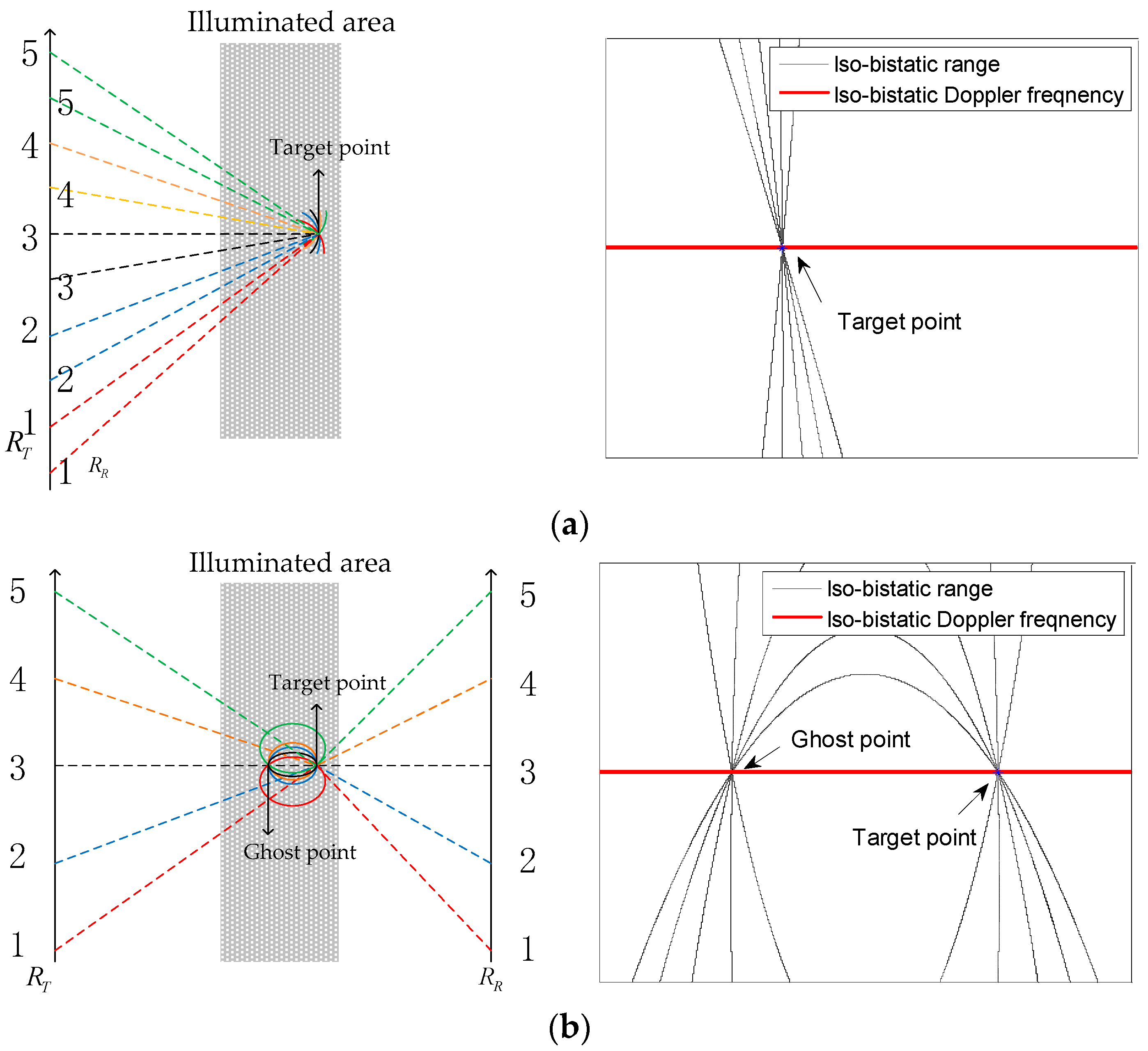
2.3. Bistatic Range History

An important difference in the forward bistatic SAR to that in the backward bistatic SAR is the existence of ghost effect, which will be explained by the range-history analysis as follows. At cross-range time $\eta$, the bistatic range $R_{bi}(\eta )$ is the summarization of the distances of the transmitter and the receiver to the target $(x,y,z)$:

$$R_{bi}(\eta )=\sqrt{{(x-x_{T\eta })}^2+{(y-y_{T\eta })}^2+{(z-H)}^2}+\sqrt{{(x-x_{R\eta })}^2+{(y-y_{R\eta })}^2+{(z-H)}^2}$$

(11)

It is clear that the iso-bistatic range $R_{bi}(\eta )$ surface in 3D space forms an ellipsoid with the transmitter and receiver at two foci. As the baseline between the transmitter and receiver decreases, the ellipsoid surface approaches a spherical surface. The intersection curve of the iso-bistatic range $R_{bi}(\eta )$ surface with the ground can be written as, setting z = 0

$$R_{bi}(\eta )=\sqrt{{(x-x_{T\eta })}^2+{(y-y_{T\eta })}^2+H^2}+\sqrt{{(x-x_{R\eta })}^2+{(y-y_{R\eta })}^2+H^2}$$

(12)

where $(x_{T\eta },y_{T\eta },H)$ and $(x_{R\eta },y_{R\eta },H)$ are the positions of the transmitter and receiver, respectively, as a function of cross-range time $\eta$. Though the iso-bistatic range forms an ellipsoid surface for the target P at any given cross-range time $\eta$, there exists a difference in the backward bistatic and forward bistatic modes that should be noted. In the backward bistatic, only one intersection curve is confined in the imaging scene. In contrast, in the forward incident plane bistatic mode, there are two intersecting curves in the imaging scene. The above scenario ranges are depicted in Figure 3. It can be clearly seen that the point P’ has the same bistatic range as the target point P in the forward vertical profile, which does not occur in the backward bistatic mode. If the point P’ has dual bistatic range histories with the target point during the whole observation time, the point P’ will induce a “false or ghost” in the focused imaging.

To further explore the properties of the bistatic range histories of the point $P{}^{\prime }(x_{P{}^{\prime },}{y}_{P{}^{\prime }})$ and target point $P(x_{P,}{y}_P)$, the iso-bistatic range and iso-bistatic Doppler frequency during the entire synthetic aperture time are depicted in Figure 4. Note that for the backward bistatic mode (Figure 4a), as both platforms move synchronously, all intersecting curves cross at one point, the target position. For the forward bistatic modes (Figure 4b), the intersecting curves meet in two points P and P′, due to equal bistatic range histories. The two range histories, Doppler histories, are equal, creating dual but identical targets in the data domain, so that a “ghost target” may appear in the focused image. It is the difference of the projection rule that the difference between the backward and forward bistatic SAR.

In the forward bistatic mode, the following equations can be sued to locate the position of the ghost P’ of a certain target P.

Plane Assumption:

$$Z_R=0$$

(13a)

Ellipsoid

$$R_{bi}({\eta }_i)=R_{bi\_P}({\eta }_i)$$

(13b)

where $R_{bi}$ is the bistatic range to the point in the imaging scene, $R_{bi\_P}$ is the bistatic range to the target point and ${\eta }_i$ is the instantaneous azimuth time, slow time, during the target exposure period. Plane assumption means only the points on the earth plane are considered. The ellipsoid equation means that the bistatic range of ghost point is equal to the bistatic range of target point in the whole observation time, which is often selected to increase the prediction accuracy of the position of ghost point.

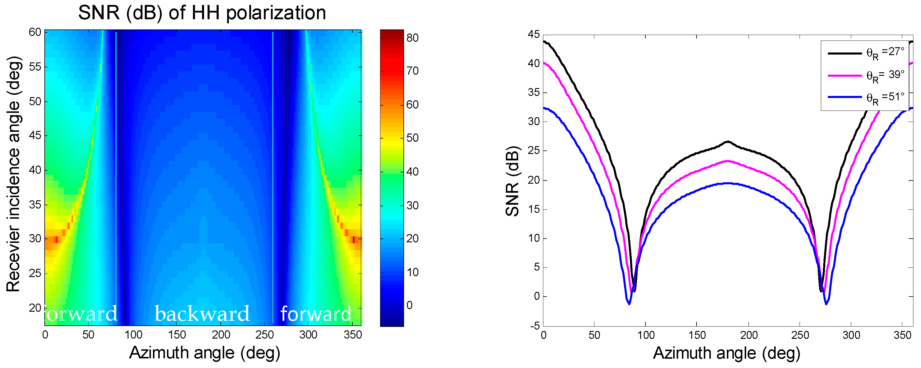
2.4. Bistatic Signal to Noise Ratio (SNR)

From the radar equation, the SNR of a SAR after signal processing is shown as:

$$SNR=\frac{P_T{G}_T{G}_R{\sigma }_{qp}^{\mathrm{o}}{A}_{cell}{\lambda }^2{T}_a{D}_c}{{(4\pi )}^3{R}_T^2{R}_R^{2}Lk{T}_R{F}_n}$$

(14)

where $P_T$ is the transmitter peak power; $G_T$ and $G_R$ are antenna gains of the transmitter and the receiver, respectively; $\lambda$ is the wavelength; $T_a$ is the integration time; $D_c$ is the duty cycle; $R_T$ and $R_R$ are the slant ranges of the transmitter and the receiver; $L$ is the energy loss during propagating; $k$ is Boltzmann’s constant; $T_R$ is the receiver noise temperature; $F_n$ is the receiver noise factor and ${\sigma }_{qp}^{°}$ is the normalized radar cross section or the scattering coefficient, with subscripts q and p denoting the transmitting and receiving polarizations, respectively.

2.5. Back-Projection Algorithm

The back-projection (BP) focusing algorithm is an autocorrelation process in the time-domain. In the BP algorithm, each received radar echo is processed and back-projected to all the imaged ground pixels. Each pixel is thus assigned a value by interpolating the pulse-echo at the time delay corresponding to the range between the pixel and the antenna. Each pixel value is accumulated as more incoming radar echoes are processed until all echoes have been processed and the final resolution achieved [18]. The BP algorithm is adopted in this study for the purpose of simulation because its focusing accuracy remains good regardless of the carrier wavelength, the desired resolution, the scene size or the imaging configuration and it is applicable to an arbitrary SAR moving path without prior assumptions.

3. Results and Discussion

For the purpose of simulation and to be more practical, we adopt the system parameters from SAOCOM-CS mission [22,23], as given in

Table 1. Key simulation parameters.

	Parameter	Symbol	Value
System parameters	Chirp bandwidth	$B$	45 MHz
	Processed Doppler bandwidth	$B_a$	1050 Hz
	Center frequency	$f_c$	1275 MHZ
	Wavelength	$\lambda$	23 cm
	Integration time	$T_a$	10 s
	Transmitter peak power	$P_T$	3.1 kW
	Antenna gain of transmitter	$G_T$	55 dB
	Antenna gain of receiver	$G_R$	50 dB
	Receiver noise temperature	$T_R$	300 K
	Receiver noise figure	$F_n$	4.5 dB
	Propagation losses	$L$	3.5 dB
	Duty cycle	$D_c$	0.05
Motion parameters	Orbit height	$H$	619.6 km
	Transmitter incidence angle	${\theta }_T$	29.55°
	Transmitter azimuth angle	${\phi }_T$	0°
	Flight velocity	$v$	7545 m/s

. In SAOCOM-CS mission, the bistatic incidence angle range is 20.7~38.4°. In our simulation, the incidence angle from the transmitter is selected as central incidence angle 29.55°.

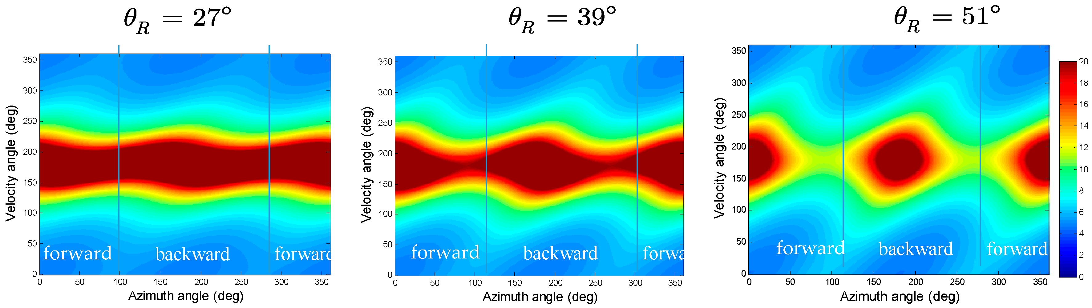
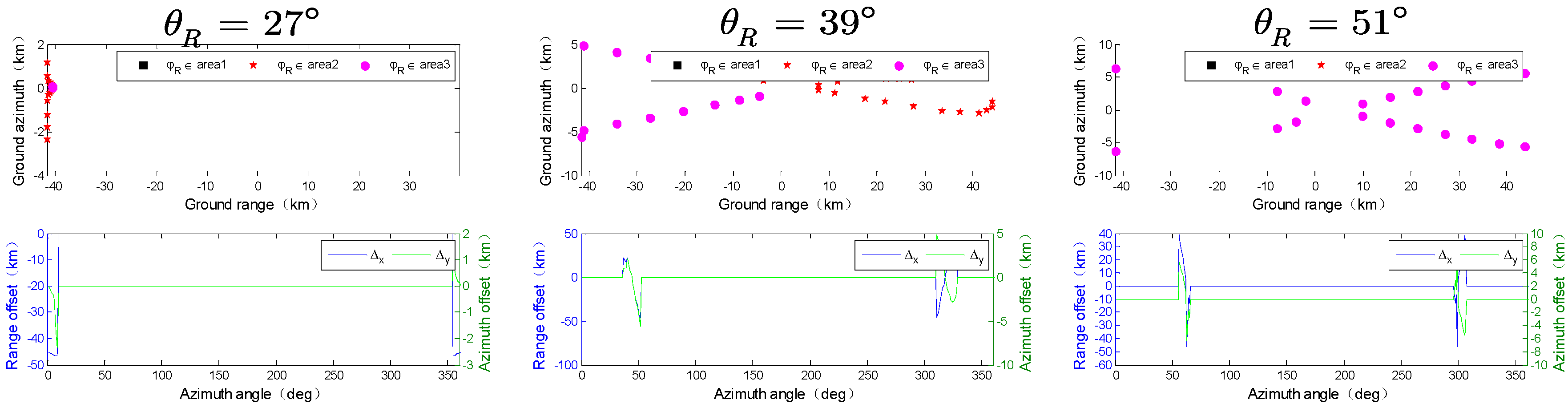
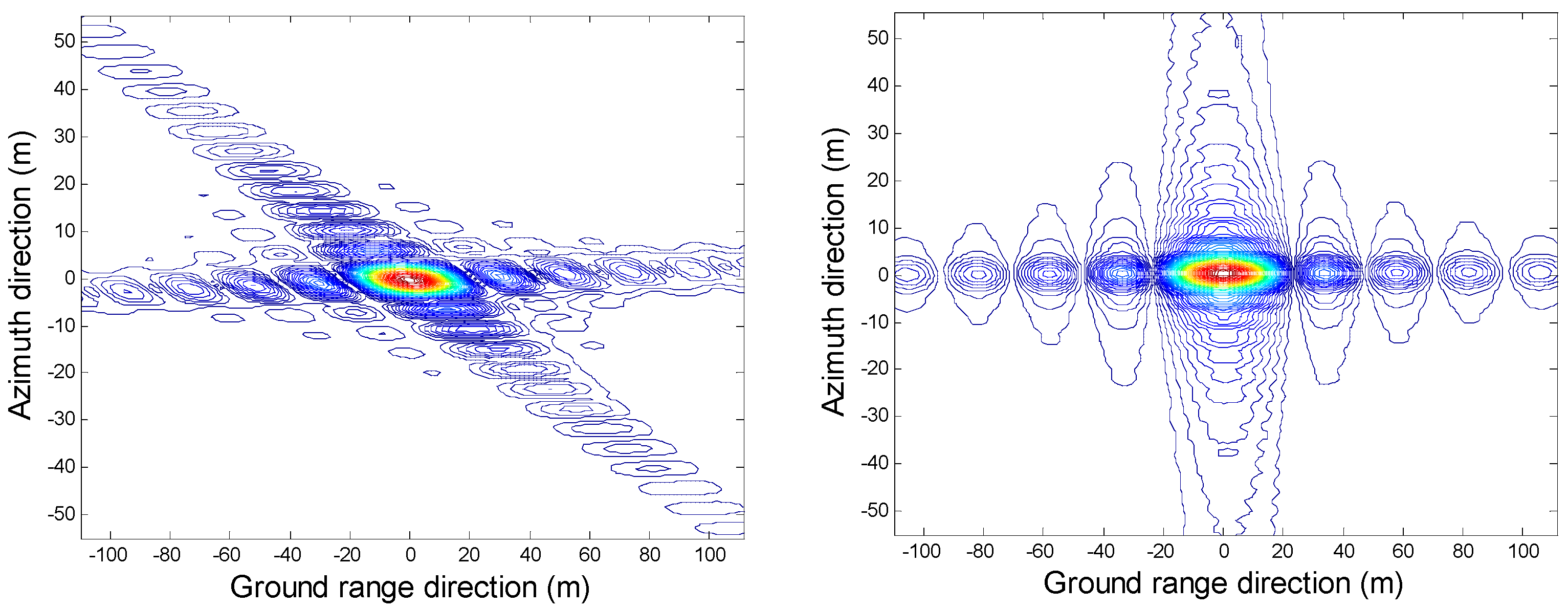
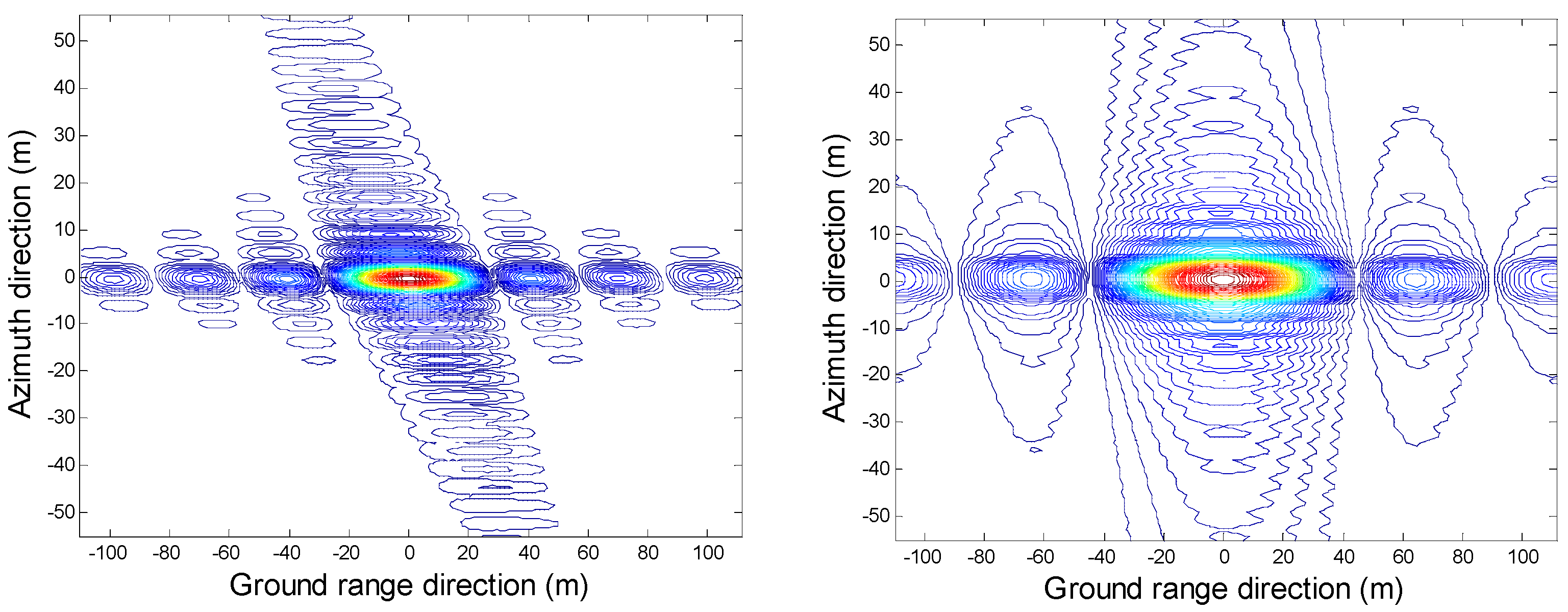
3.1. Imaging Property of Backward and Forward Bistatic SAR

In this subsection, the imaging property of backward and forward bistatic SAR will be analyzed. This system works in the receiver incidence angle between 21° and 57° with 7 beams in total (3 degrees on the left and right sides of the beam center) and its corresponding ground range resolution is shown in Figure 5.

It can be seen that the ground range resolution in the backward mode is similar to monostatic SAR and that is beneficial for imaging. In addition, only in the forward scattering zone, the ground range resolution deteriorates and the phenomenon is more obvious as the incidence angle differences between the transmitter and the receiver become small, particularly near the specular region. These properties can be explained by Equation (3). In the forward specular bistatic, the transmitter and the receiver are symmetrical about the center region within the imaging scene. This symmetry causes the two opposite direction vectors in the x-axis to counteract each other and the resolution becomes extremely poor. As the angular difference between the transmitter and receiver becomes larger, the ground range resolution changes are mitigated and improve considerably. Thus, conclusions can be drawn that the ground range resolution in the backscattering zone is superior to that in the forward backscattering zone with a certain incidence angle. To improve the ground range resolution, the receiver incidence angle should be selected away from the transmitter incidence angle and the azimuth angle should be increased as much as possible. In addition, special attention should be paid to avoid the approximately symmetrical imaging configuration in the forward bistatic SAR.

Figure 6 shows the azimuth resolution with respect to the velocity direction angle $\beta$ and azimuth angle ${\phi }_R$. It is seen that the azimuth resolution has a slight change when $\beta =0^{°}$, since the two SAR platforms move in the same direction with a parallel track. When the velocity angle is close to 180 degrees, the azimuth resolution diverges, because the angular velocity vectors $w_T(\eta )$ and $w_R(\eta )$ are in opposition, which therefore is not recommended in bistatic SAR. The influence of the velocity direction angle is dominant and the receiver incidence angle adds to the effect. Conclusions that the opposite velocity vectors are not desirable even though the azimuth resolution becomes better as the receiver incidence angle changes. Except in the case of velocity angle near to 180 degrees, there is not much difference for the azimuth resolution for backward and forward bistatic SAR.

In most practical case, the velocity angle is set zero, which means a parallel track. The ground range and azimuth resolutions, resolution direction angle and the ground resolution cell area with respect to the azimuth angle and the receiver incidence angle, with ${\theta }_T={29.55}^{°}$ and $\beta =0^{°}$ are plotted in Figure 7. Figure 7a shows that the azimuth resolution changes slightly in the whole scattering zone when $\beta =0^{°}$ but it suffers degradation when ${\phi }_R$ is near ${90}^{°}$ and ${270}^{°}$ because the sum of angular velocity units $w_T(\eta )$ and $w_R(\eta )$ (see Equation (6)) is smaller. Figure 7b shows that the directions of the two resolutions are almost collinear in some regions in the forward scattering zone which causes defocus in the final image. Figure 7c also indicates the same trend; it can be seen that the areas with an orthogonal resolution direction angle are not strictly in conformity with the area with the smallest ground resolution cell and it is also influenced by the two ground resolutions. In some regions in the forward bistatic mode, the resolution cell is totally lost and should be avoided when designing the imaging geometric parameters.

Then, the simulated forward quasi-specular bistatic SAR (${\theta }_R={27}^{°}$ and ${\phi }_R=0^{°}$) image further verifies the above observation. From Figure 8 and Figure 9, in the forward quasi-specular bistatic mode, the azimuth resolution is fine while the ground range resolution deteriorates rapidly. The simulated results are consistent with the above analysis. It should be note that the forward specular bistatic is not recommended for forward imaging in view of the resolution.

It is seen that there is “ghost target” in the range direction caused by the same bistatic range histories. It can be explained by Equation (5), targets and the “ghost targets” follow the iso-range histories so that the signal returns may accumulate to the location where no actual target exists, which means that except for the real targets, the “ghost target” will be created in the focusing image. Assume the antenna pattern of the transmitter and receiver are strictly controlled. In order to clearly show the characteristics of the ghost effect, the ghost positions of the target (5000, 0, 0) in different configurations are calculated according Equation (13). The whole imaging scene is divided into three parts as shown in Figure 10. The black block presents the backward zone, the red block presents the area with ${\phi }_R\in (0°,90)\cup (270°,360°)$ and the pink block is the remainder of the forward zone.

Just three receiver beams are shown in Figure 11 to illustrate this trend. The figures represent the offset of the ghost point in the range direction and the azimuth direction as the azimuth angle of the receiver changes from $0°$ to $360°$. If the real target point does not appear offset in the two-dimensional direction, it is not displayed in the figure. Not unexpectedly, ghost effect does not appear in the backward scattering zone. The ghost area moves as the variation of the incident difference angle of the transmitter and the receiver. When the difference angle is small, the ghost effect is significant in the area where the azimuth angle is small, and as the difference angle becomes large, this phenomenon is gradually transferring to a larger azimuth angle. Enlarging the difference angle of the transmitter and receiver is beneficial to obtain a wider imaging scene. In addition, the offset along azimuth direction is one magnitude less than range direction offsets which can be ignored in some cases.

For the incidence plane bistatic, the positions of the target and the ghost are symmetrical to the center of the scene, as shown in Figure 12. The ghost-free scene width W can be calculated by (15). W means the width starting from the left boundary of the co-illumination area.

$$W=\{\begin{array}{c}\left|X_l+X_r-2X_c\right|,X_c\in (X_l,X_r)\\ X_l-X_r,X_c\notin (X_l,X_r)\end{array}$$

(15)

where $X_c=\frac{X_T+X_R}{2}$ is the center of the scene, $X_l=\max (X_{tl},X_{rl})$ is the left boundary of the co-illumination area and $X_r=\min (X_{tr},X_{rr})$ is the right boundary of the co-illumination area. $X_{tl},X_{rl},X_{tr},X_{rr}$ are the boundary lines of the transmitter illumined area and receiver illumined area, respectively.

$$\{\begin{array}{l}{X}_{tl}=-H_T[\tan {\theta }_T-\tan ({\theta }_T-\Delta {\theta }_T)]\\ X_{rl}=-H_R[\tan ({\theta }_R+\Delta {\theta }_R)-\tan {\theta }_R]\\ X_{tr}=H_T[\tan ({\theta }_T+\Delta {\theta }_T)-\tan {\theta }_T]\\ X_{rr}=H_R[\tan {\theta }_R-\tan ({\theta }_R-\Delta {\theta }_R)]\end{array}$$

(16)

where ${\theta }_R={\theta }_T+\Delta \theta$, $\Delta \theta$ is the difference angle of the transmitter angel receiver. For example, in this case, while $\Delta \theta =4°$, that is ${\theta }_R=33.55°$, $X_l=-41.7\mathrm{km}$. The 57 km imaging range from the left boundary of the co-illumination area is obtained and 15.3 km on each side with the transmitter center beam as the center, which is enough for many applications. Thus, in order to avoid ghost effect caused by the bistatic geometry, the difference angle should be more than $4°$.

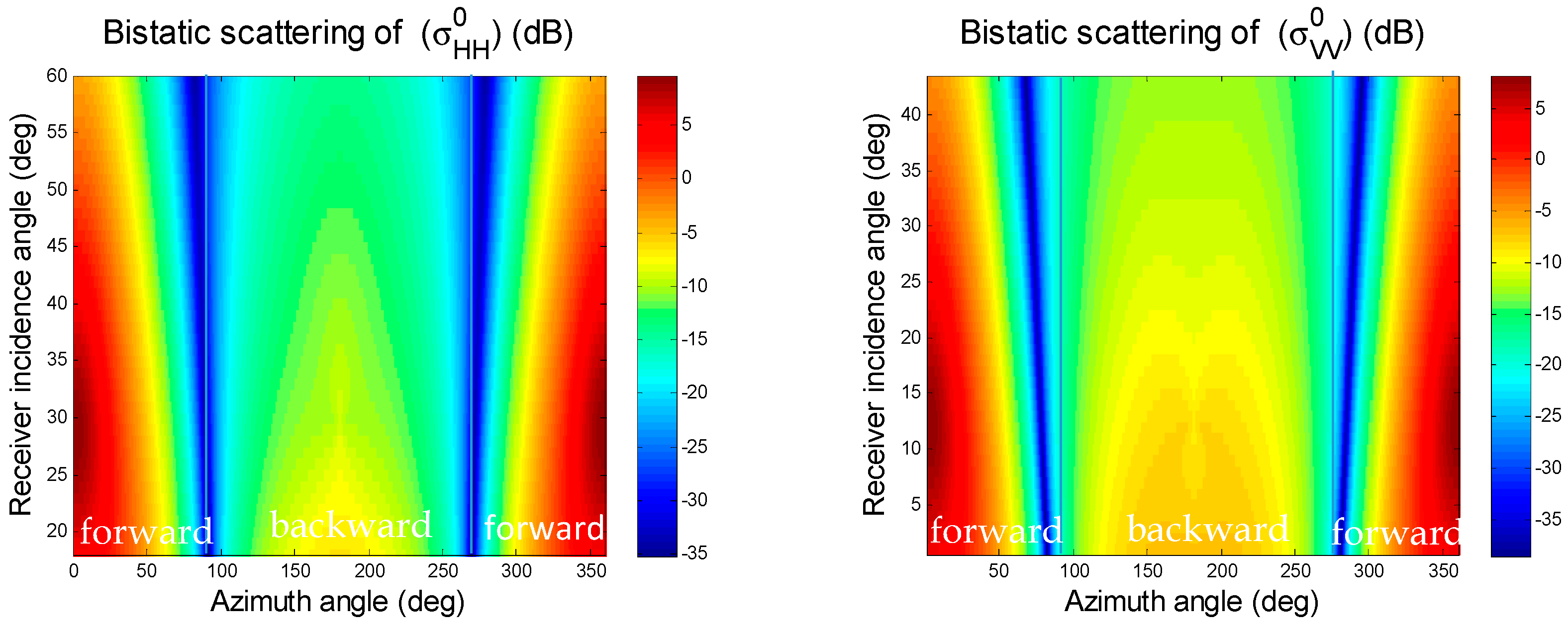
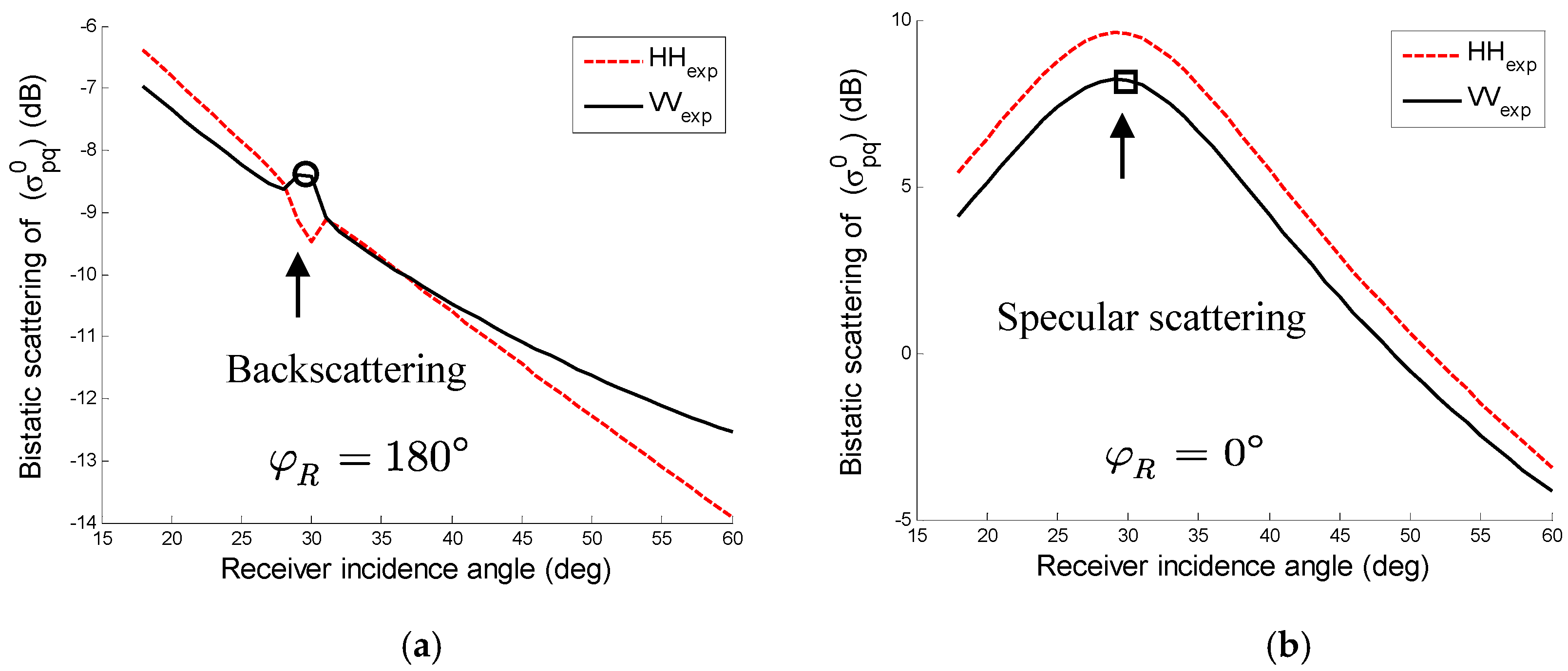
3.2. Power Considerations of Backward and Forward Bistatic SAR

In the imaging performances, the resolution and SNR are considered simultaneously. To demonstrate the SNR of backward and forward bistatic SAR, first, we compute the scattering coefficients for roughness of correlation length $l=\lambda$ and rms height $s=\lambda /10$ ($\lambda$ = radar wavelength) with exponential ACF by advanced integral equation model (AIEM) [26]. The AIEM can be represented as follows:

$${\sigma }_{pp}=AIEM(f_c,{\theta }_T,{\theta }_R,{\phi }_R,{\epsilon }_r,rms,l,pp)$$

(17)

where ${\epsilon }_r=12-1.2j$ is the complex dielectric constant, ${\sigma }_{pp}$ is the normalized radar scattering cross section area of $pp$ polarization.

In Figure 13, it can be observed that the bistatic scattering of the HH polarization and VV polarization are quite similar and has stronger returns in the forward scattering zone compared to that in the backward scattering zone. It is noted that there exist dips in the azimuthal plane when ${\phi }_R$ is near ${90}^{°}$ and ${270}^{°}$. It can be clearly seen that the bistatic forward scattering observations provide a larger spacing between the HH polarization and VV polarization (shown as the square mark in Figure 14b) than that in the backward bistatic zone such as the monostatic observations (shown as the circle mark in Figure 14a), which means that the bistatic forward mode provide more target information than the bistatic backward mode.

Figure 15 shows the simulated SNR under HH polarization with respect to ${\theta }_R$ and ${\phi }_R$. It can be seen, the SNR in the forward imaging zone is mostly better than that in backward imaging zone. The SNR gaps appear at nearly ${\phi }_R={90}^{°}$ and ${\phi }_R={270}^{°}$, which should be paid more attention when singing motion parameters. Both the resolution and the SNR are pretty important performance indexes when designing motion parameter, which should be balanced.

3.3. Chaos Particle Swarm Optimization

As we mentioned before, the main imaging performance in bistatic SAR are range resolution ${\rho }_{gr}$, azimuth resolution ${\rho }_{ga}$, resolution angle $\psi$, resolution cell $A_{cell}$ and $SNR$, which are nonlinear functions of ${\theta }_R$, ${\phi }_R$ and $\beta$. Given a specific application, the desired imaging performance can be set ${\rho }_{grD}$, ${\rho }_{gaD}$, ${\psi }_D$, $A_{cellD}$ and $SN{R}_D$. Therefore, the mission design process can be considered as an NES with three independent variables.

$$F(x)=0$$

(18)

where $0={(0,0,0)}^T$ is zero vectors and $F(x)$ is the system of nonlinear equations, which is given by

$$F(x)=\left[\begin{array}{c}{f}_1(x)\\ f_2(x)\\ f_3(x)\\ \begin{array}{l}{f}_4(x)\\ f_5(x)\end{array}\end{array}\right]=\left[\begin{array}{c}{\rho }_{gr}({\theta }_R,{\phi }_R,\beta )-{\rho }_{grD}\\ {\rho }_{ga}({\theta }_R,{\phi }_R,\beta )-{\rho }_{gaD}\\ \psi ({\theta }_R,{\phi }_R,\beta )-{\psi }_D\\ A_{cell}({\theta }_R,{\phi }_R,\beta )-A_{cellD}\\ SNR({\theta }_R,{\phi }_R,\beta )-SN{R}_D\end{array}\right]=0$$

(19)

where $x={({\theta }_R,{\phi }_R,\beta )}^T\in D$ is the decision vector and $D$ is the decision space of three dependent variables, which is given by

$$D=\{\begin{array}{l}{\theta }_R\in (0°,90°)\\ {\phi }_R\in [-90°,90°)\\ \beta \in [0°,360°)\end{array}$$

(20)

Particle swarm optimization (PSO) [27] is a bionic optimization algorithm based on observations of the foraging process of animals such as bird flocking and fish schooling. PSO is initialized with a group of random particles and then searches for optima by the updating generations. In every iteration, each particle quality is evaluated by two “best” values which calculated by the fitness function. The first value is the best individual solution which presents the own flying experiences and another is the global best solution which presents its companions flying experiences. Then, each particle updates velocity according to these two values to determine the distance and direction of flying. Finally, the global best solution in the search space is obtained. Compared with other classic methods, such as genetic algorithm (GA), the advantages of PSO are that PSO is easy to implement and there are a few parameters to adjust; and the particles in PSO have memory so knowledge of good solutions is retained by all particles; in addition, PSO is a one-way information sharing mechanism, all particles tend to converge to the best resolution quickly. However, the performance of both PSO and GA realty depends on their parameters and they often suffer the problem of being trapped in local optima so as to be premature convergence [28]. Chaos particle swarm optimization (CPSO) combines chaos optimization with the PSO. For a given energy or cost function, by following the ergodic, stochastic and regular property of chaotic variables, a chaotic dynamic system may eventually reach the global optimum or its good approximation with high probability.

It should be noted the five nonlinear equations in (19) with different dimension should be normalized respectively before calculating fitness. The basic steps of CPSO are described as follows:

Step 1: construct the imaging NES

Step 1.1: input the desired imaging performance

Step 1.2: construct the imaging NES

Step 1.3: construct the energy function

The energy function can be obtained and the problem turns from solving NES to find the minimal value of the energy function.

$$\mathsf{\Phi }(x)=\min {\displaystyle \sum _{i=1}^5{f}^{\ast }{}_i^2(x)}$$

(21)

where $f^{\ast }(x)$ is normalized function. When $\mathsf{\Phi }(x_0)<\epsilon$, the optimal solution $x_0={({\theta }_{R0},{\phi }_{R0},{\beta }_0)}^T$ is selected.

Step 2: Initialization

Step 2.1: Initialize the position $X_i$ of particles by chaos

(1)

Initialize a vector $Z=(z_1,z_2,\cdots ,z_m)$ each component using a random number in the range [0, 1] and produce m-D chaos queues $z_1,z_2,\cdots ,z_{2N}$ by 2N iteration of Logistic equation.

(2)

Map the chaos queues into the decision space of the parameters $x_i\in (a_i,b_i)$ according the following equation to obtain 2N initialized positions

$$Z\to X:x_i=a_i+(b_i-a_i)z_i$$

(22)

(3)

Calculate the fitness values of the vectors using the fitness function and select the best N solutions as the initial positions of N particles.

$$fitness=\mathsf{\Phi }(x)$$

(23)

Step 2.2: Initialize the velocity $V_i$ of particle randomly in the range of $(0,V_{\max })$

Step 2.3: Initialize the local-best position $pbest$ and the global-best position $gbest$

Step 3: Repeat until the $\mathsf{\Phi }(gbes{t}_i)<\epsilon$

Step 3.1: Update each particle’s velocity and position:

$${\mathrm{v}}_{\mathrm{i}}^{\mathrm{k}}=w{\mathrm{v}}_{\mathrm{i}}^{\mathrm{k}-1}+c_1{r}_1(pbes{t}_i-x_i^{k-1})+c_2{r}_2(gbest-x_i^{k-1})$$

(24)

$$x_i^k=x_i^{k-1}+v_i^{k-1}$$

(25)

$$w=w_{\max }-\frac{run(w_{\max }-w_{\min })}{ru{n}_{\max }}$$

(26)

Step 3.2: Update each particle’s $pbes{t}_i$ if the $\mathsf{\Phi }(x_i^k)<\mathsf{\Phi }(pbes{t}_i)$

Step 3.3: Update each particle’s $gbes{t}_i$

Step 4: Optimize $gbes{t}_i$ by chaos search

Step 4.1: Map the $gbest$ into the chaos queues:

$$X\to Z:z_i=(gbes{t}_i-a_i)/(b_i-a_i)$$

(27)

Step 4.2: Produce the next chaos queues:

$$Z^k\to Z^{k+1}:z_i^{k+1}=4z_i^k(1-z_i^k)$$

(28)

Step 4.3: Map the $z_i^{k+1}$ into $gbes{t}_i$ using Equation (22):

$$Z\to X:gbes{t}_i=a_i+(b_i-a_i)z_i$$

(29)

Step 4.4: Evaluate the fitness value in the problem space during chaotic search and get the best solution $gbes{t}_i$

Step 5: If $\mathsf{\Phi }(gbes{t}_i)>\epsilon$, $t=t+1$ and go back to step 3. Otherwise stop and output the $gbes{t}_i$ found best so far.

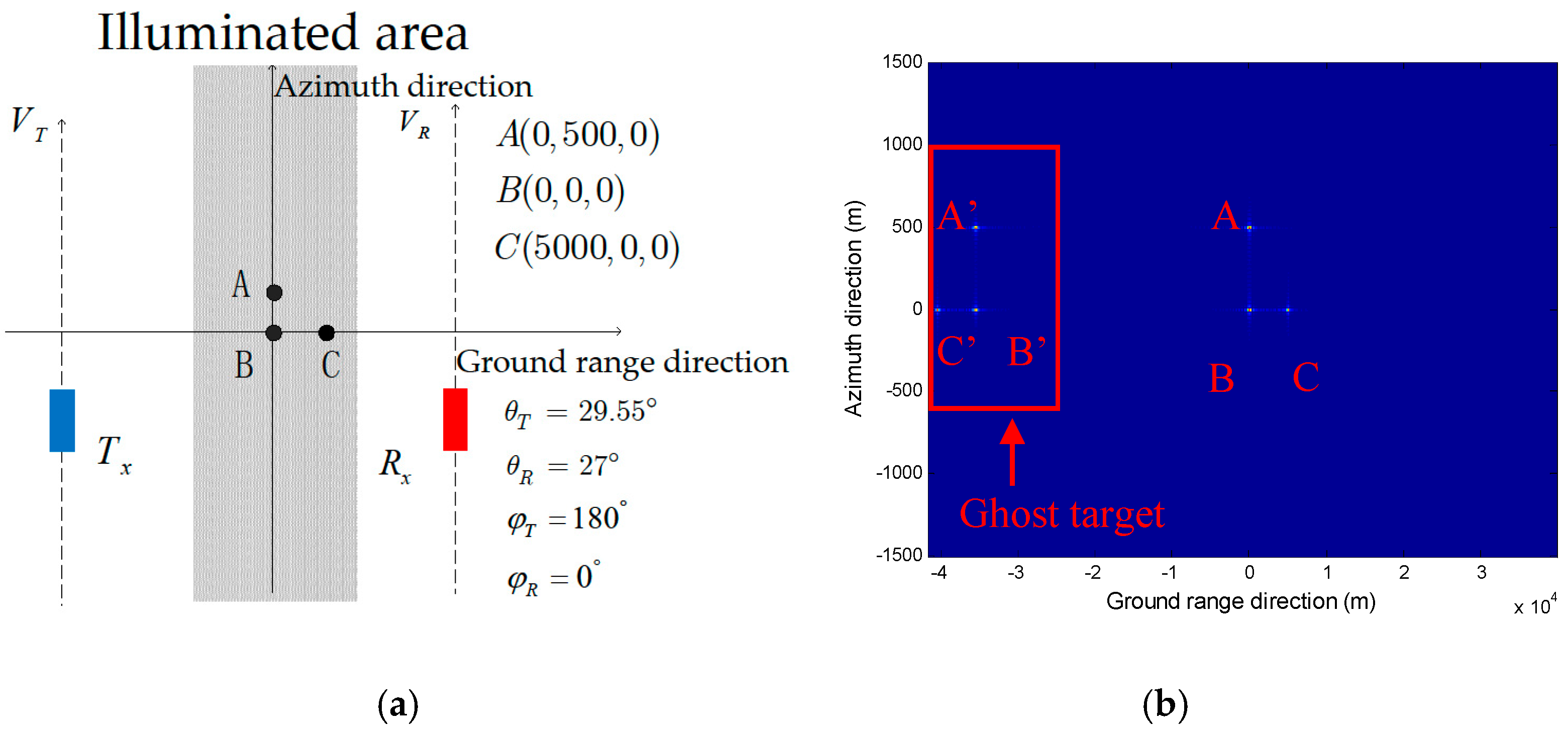
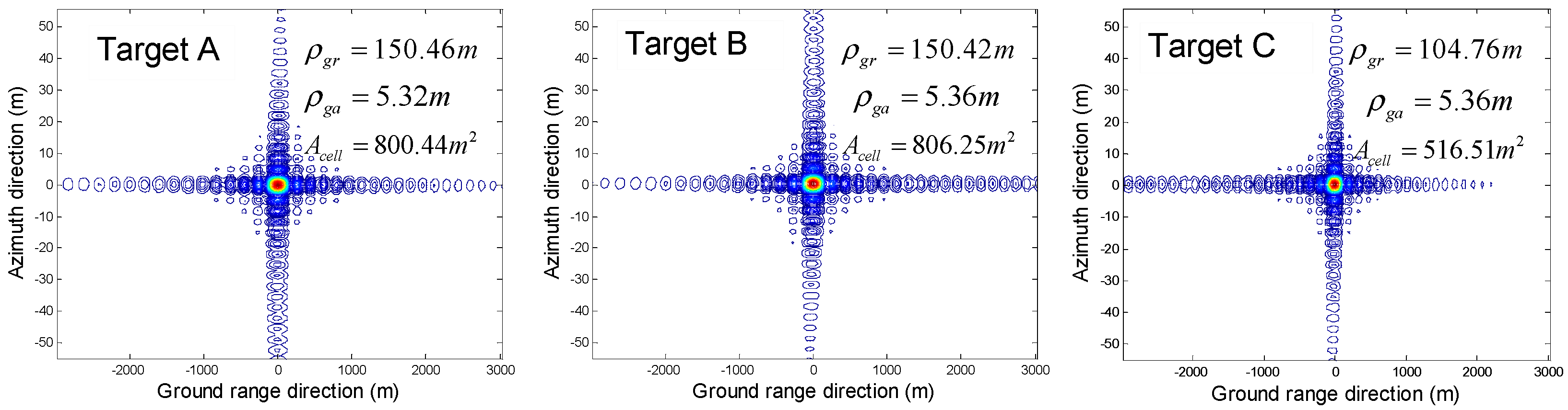
3.4. Simulation and Results

The parameters used in CPSO are listed in

Table 2. Key parameters relevant to three bistatic formations.

Parameter	Symbol	Value
Population size	N	200
Particle size	m	3
Predetermined accuracy	$\epsilon$	0.001
Maximum weight	$w_{\max }$	0.9
Minimum weight	$w_{\min }$	0.4
Maximum velocity	$V_{\max }$	π/16
Acceleration coefficients 1	$c_1$	2
Acceleration coefficients 2	$c_2$	2

.

Table 3. Key parameters relevant to three bistatic formations.

Desired Imaging Performance					Optimal Solutions (°)			Measured Performance
${\mathit{\rho }}_{\mathit{g}\mathit{r}\mathit{D}}$ (m)	${\mathit{\rho }}_{\mathit{g}\mathit{a}\mathit{D}}$ (m)	${\mathit{\psi }}_{\mathit{D}}$ (°)	${\mathit{A}}_{\mathit{c}\mathit{e}\mathit{l}\mathit{l}\mathit{D}}$ (m2)	$\mathit{S}\mathit{N}{\mathit{R}}_{\mathit{D}}$ (dB)	${\mathit{\theta }}_{\mathit{R}}$	${\mathit{\phi }}_{\mathit{R}}$	$\mathit{\beta }$	${\mathit{\rho }}_{\mathit{g}\mathit{r}}$ (m)	${\mathit{\rho }}_{\mathit{g}\mathit{a}}$ (m)	$\mathit{\psi }$ (°)	${\mathit{A}}_{\mathit{c}\mathit{e}\mathit{l}\mathit{l}}$ (m2)	$\mathit{S}\mathit{N}\mathit{R}$ (dB)
11.65	4.56	67.45	57.45	22.89	57.19	11.13	5.24	11.93	4.58	66.02	60.45	23.58
15.17	4.66	90.00	70.77	28.23	52.29	0.20	3.04	15.45	4.98	91.06	76.95	28.59
18.26	4.73	79.16	87.93	31.53	47.74	3.36	8.36	17.69	4.75	75.26	86.89	31.48
29.61	4.78	90.00	141.6	38.23	40.52	0.15	2.11	33.26	4.92	86.34	163.97	38.74

shows 4 cases with different desired imaging performance.

The optimal solutions can be obtained by CPSO, then BP focusing algorithm is utilized to test the optimal solutions. The optimal solutions obtained by CPSO under a desired imaging performances and their corresponding measured imaging performances are listed in Table 3.

In Table 3, the measured performances from the simulation results are similar to expectations. The slight deviation may be due to the randomness of the initial value of CPSO. Figure 16 shows the simulated point target responses of the optimal resolutions. The results show CPSO can determine the imaging geometry quickly and accurately and meet most accuracy requirements.

4. Conclusions

In this work, the geometric properties and power considerations of the backward and forward bistatic SAR are analyzed in a formation mode. In addition, the focus is on the forward bistatic configuration which has been proven to be beneficial for remote sensing applications. As predicted by the range history analysis and verified by the BP imaging simulation results, the bistatic range history phenomenon that introduces “ghost targets” exists when the imaging area is across the specular region. That drawback should be avoided by limiting the illumination area beside the specular region rather than across it. By enlarging the difference in the incidence angles of the transmitter (θ_T) and receiver (θ_R), the ghost-free area can be broadened for practical observations. The two-dimensional ground resolution properties are also analyzed. From the view of realizing a sufficiently high resolution, the quasi-specular forward imaging geometry should also be avoided, as the ground range resolution deteriorates badly in this case. The Azimuth resolution variation is relatively insignificant as long as the velocity directions of the transmitter and receiver are not notably different. Then, based on the considerations of the range ambiguity effect, the ground resolution cell area size, along with the SNR, suggestion on the forward bistatic SAR imaging geometry design can be concluded: a sufficiently large difference in the transmitting and receiving incidence angle (θ_T and θ_R, θ_R > θ_T) should be guaranteed near the incident plane (φ_Rϵ(φ_T-180° − Δ, φ_T-180° + Δ)), for ghost-free imaging and achieving good balance between fine resolution and high SNR, as well as obtaining richer scattering features from earth surfaces. Finally, the CPSO is used to find the optimal angle combinations under a given resolutions and SNR. In the simulation, the resolutions and SAR measured is similar to the desired values, which demonstrate the effectiveness of the algorithm. The analysis and discussions on the formation bistatic SAR geometry can be advantageous and informative for future forward bistatic SAR system developments.

References

1. Krieger, G.; Hajnsek, I.; Papathanassiou, K.P.; Younis, M.; Moreira, A. Interferometric synthetic aperture radar (SAR) missions employing formation flying. Proc. IEEE 2010, 98, 816–843. [Google Scholar] [CrossRef] [Green Version]
2. Erten, E.; Rossi, C.; Yuzugullu, O. Polarization impact in tandem-X data over vertical-oriented vegetation: The paddy-rice case study. IEEE Geosci. Remote Sens. Lett. 2015, 12, 1501–1505. [Google Scholar] [CrossRef]
3. Yang, X.F.; Du, Y.L.; Li, Z.W.; Chen, K.S. Investigation of bistatic radar scattering from sea surfaces with breaking waves. In Proceedings of the 2017 IEEE International Geoscience and Remote Sensing Symposium (IGARSS), Fort Worth, TX, USA, 23–28 July 2017; pp. 1502–1503. [Google Scholar]
4. Moreira, A.; Gerhard, K.; Hajnsek, I.; Papathanassiou, K.; Younis, M.; Dekker, P.L.; Huber, S.; Villano, M.; Pardini, M.; Michael, E.; et al. Tandem-L: A highly innovative bistatic SAR mission for global observation of dynamic processes on the Earth’s surface. IEEE Geosci. Remote Sens. Mag. 2015, 3, 8–23. [Google Scholar] [CrossRef]
5. Guerriero, L.; Pierdicca, N.; Pulvirenti, L.; Ferrazzoli, P. Use of Satellite Radar Bistatic Measurements for Crop Monitoring: A Simulation Study on Corn Fields. Remote Sens. 2013, 5, 864–890. [Google Scholar] [CrossRef] [Green Version]
6. Zeng, J.Y.; Chen, K.S. Theoretical Study of Global Sensitivity Analysis of L-band Radar Bistatic Scattering for Soil Moisture Retrieval. IEEE Geosci. Remote Sens. Lett. 2018, 1–5. [Google Scholar] [CrossRef]
7. Fernandez, P.D.; Cantalloube, H.; Vaizan, B.; Krieger, G.; Horn, R.; Wendler, M.; Giroux, V. ONERA-DLR bistatic SAR campaign: Planning, data acquistiton, and first analysis of bistatic scattering behaviour of natural and urban targets. IEE Proc. Radar Sonar Navig. 2006, 153, 214–223. [Google Scholar] [CrossRef]
8. Cardillo, G.P. On the use of the gradient to determine bistatic SAR resolution. In Proceedings of the Antennas and Propagation Society International Symposium, Dallas, TX, USA, 7–11 May 1990; pp. 1032–1035. [Google Scholar]
9. Zeng, T.; Cherniakov, M.; Long, T. Generalized approach to resolution analysis in BSAR. IEEE Trans. Aerosp. Electron. Syst. 2005, 41, 461–474. [Google Scholar] [CrossRef]
10. Ender, J.H.G. The meaning of k-space for classical and advanced SAR-techniques. In Proceedings of the Second International Symposium Physics in Signal & Image Processing (PSIP’2001), Marseille, France, 23–24 January 2001. [Google Scholar]
11. Moccia, A.; Renga, A. Spatial resolution of bistatic synthetic aperture radar: Impact of acquisition geometry on imaging performance. IEEE Trans. Geosci. Remote Sens. 2011, 49, 3487–3503. [Google Scholar] [CrossRef]
12. Jiang, Y.; Wang, Z. Analysis for Resolution of Bistatic SAR Configuration with Geosynchronous Transmitter and UAV Receiver. Int. J. Antennas Propag. 2013, 6, 245–253. [Google Scholar] [CrossRef]
13. Sun, Z.C.; Wu, J.J.; Pei, J.F.; Li, Z.Y.; Huang, Y.L.; Yang, J.Y. Inclined geosynchronous spaceborne—Airborne bistatic sar: Performance analysis and mission design. IEEE Trans. Geosci. Remote Sens. 2016, 54, 343–357. [Google Scholar] [CrossRef]
14. Wang, R.; Deng, Y.K.; Loffeld, O.; Nies, H.; Walterscheid, I.; Espeter, T.; Klare, J.; Ender, J.H.G. Processing the azimuth-variant bistatic SAR data by using monostatic imaging algorithms based on two-dimensional principle of stationary phase. IEEE Trans. Geosci. Remote Sens. 2011, 49, 3504–3520. [Google Scholar] [CrossRef]
15. Zeng, T.; Liu, F.; Hu, C.; Long, T. Image formation algorithm for asymmetric bistatic sar systems with a fixed receiver. IEEE Trans. Geosci. Remote Sens. 2012, 50, 4684–4698. [Google Scholar] [CrossRef]
16. Li, D.; Wang, W.; Liu, H.Q.; Cao, H.L.; Lin, H. Focusing highly squinted Azimuth variant Bistatic SAR. IEEE Trans. Aerosp. Electron. Syst. 2017, 52, 2715–2730. [Google Scholar] [CrossRef]
17. Walterscheid, I.; Ender, J.H.G.; Brenner, A.R.; Loffeld, O. Bistatic sar processing and experiments. IEEE Trans. Geosci. Remote Sens. 2006, 44, 2710–2717. [Google Scholar] [CrossRef]
18. Cassola, M.R.; Prats, P.; Krieger, G.; Moreira, A. Efficient time-domain image formation with precise topography accommodation for general bistatic SAR configurations. IEEE Trans. Aerosp. Electron. Syst. 2011, 47, 2949–2966. [Google Scholar] [CrossRef] [Green Version]
19. Shao, Y.F.; Wang, R.; Deng, Y.K.; Liu, Y.; Chen, R.; Liu, G.; Loffeld, O. Fast backprojection algorithm for bistatic SAR imaging. IEEE Geosci. Remote Sens. Lett. 2013, 10, 1080–1084. [Google Scholar] [CrossRef]
20. Vu, V.T.; Pettersson, M.I. Fast backprojection algorithms based on subapertures and local polar coordinates for general bistatic airborne sar systems. IEEE Trans. Geosci. Remote Sens. 2016, 54, 2706–2712. [Google Scholar] [CrossRef]
21. Wang, Y.; Liu, Y.Y.; Li, Z.F.; Suo, Z.Y.; Fang, C.; Chen, J.L. High-resolution wide-swath imaging of spaceborne multichannel bistatic SAR with inclined geosynchronous illuminator. IEEE Geosci. Remote Sens. Lett. 2017, 14, 2380–2384. [Google Scholar] [CrossRef]
22. Gebert, N.; Dominguez, B.C.; Davidson, M.W.J.; Martin, M.D.; Silvestrin, P. SAOCOM-CS—A passive companion to SAOCOM for single-pass L-band SAR interferometry. In Proceedings of the 2014 10th European Conference on Synthetic Aperture Radar (EUSAR), Berlin, Germany, 3–5 June 2014; pp. 1–4. [Google Scholar]
23. Bordoni, F.; Younis, M.; Cassola, M.R.; Iraol, P.P.; Dekker, P.L.; Krieger, G. SAOCOM-CS SAR imaging performance evaluation in large baseline bistatic configuration. In Proceedings of the 2015 IEEE International Geoscience and Remote Sensing Symposium (IGARSS), Milan, Italy, 26–31 July 2015; pp. 2107–2110. [Google Scholar]
24. Gebert, N.; Dominguez, B.C.; Martin, M.D.; Salvo, E.D.; Temussi, F.; Giove, P.V.; Gibbons, M.; Phelps, P.; Griffiths, L. SAR Instrument Pre-development Activities for SAOCOM-CS. In Proceedings of the 2016 11th European Conference on Synthetic Aperture Radar (EUSAR), Hamburg, Germany, 6–9 June 2016; pp. 1–4. [Google Scholar]
25. Qiu, X.L.; Ding, C.B.; Hu, D.H. Bistatic SAR Data Processing Algorithms; John Wiley & Sons: Singapore, 2013; p. 80. ISBN 9781118188088. [Google Scholar]
26. Wu, T.D.; Chen, K.S.; Shi, J.; Lee, H.W.; Fung, A.K. A study of an AIEM model for bistatic scattering from randomly rough surfaces. IEEE Trans. Geosci. Remote Sens. 2008, 46, 2584–2598. [Google Scholar] [CrossRef]
27. Coello, C.A.C.; Pulido, G.T.; Lechuga, M.S. Handling multiple objectives with particle swarm optimization. IEEE Trans. Evol. Comput. 2004, 8, 256–279. [Google Scholar] [CrossRef]
28. Liu, B.; Wang, L.; Jin, Y.H.; Tang, F.; Huang, D.X. Improved particle swarm optimization combined with chaos. Chaos Solitons Fractals 2005, 25, 1261–1271. [Google Scholar] [CrossRef]
Figure 1. Imaging geometry of bistatic SAR.
Remotesensing 10 01676 g001
Figure 2. The ground resolution cell of bistatic SAR.
Remotesensing 10 01676 g002
Figure 3. The illustration of the spherical and ellipsoid surface of the backward bistatic and forward bistatic.
Remotesensing 10 01676 g003
Figure 4. The range histories of the backward bistatic (a) and forward bistatic (b) at target P during full aperture and the numbers 1 to 5 represent different positions of the transmitter and receiver at the azimuth direction. The right column is the zoom of the target imaging scene of the left column.
Remotesensing 10 01676 g004
Figure 5. (Left): The ground range resolution with respect to the received azimuth angle φ R . (Right): The ground range resolution in different beams.
Remotesensing 10 01676 g005
Figure 6. The azimuth resolution with respect to velocity angle β and received azimuth angle φ R when θ T = 29.55 ° .
Remotesensing 10 01676 g006
Figure 7. The resolution analysis with respect to θ R and φ R . (a) Azimuth resolution; (b) Resolution direction angle; (c) Ground resolution cell when θ T = 29.55 ° .
Remotesensing 10 01676 g007
Figure 8. Imaging simulation of the forward quasi-specular bistatic. (a) Sketch; (b) Imaging result.
Remotesensing 10 01676 g008
Figure 9. Simulated point target responses of the forward quasi-specular bistatic.
Remotesensing 10 01676 g009
Figure 10. The location diagram of platforms.
Remotesensing 10 01676 g010
Figure 11. The first line indicates the location of the ghost point and the second line indicates the positional offset between the ghost target point and the real target point along range and azimuth direction when θ T = 29.55 ° .
Remotesensing 10 01676 g011
Figure 12. Ghost effect in incidence plane bistatic SAR.
Remotesensing 10 01676 g012
Figure 13. Bistatic scattering coefficients σ H H 0 and σ V V 0 when θ T = 29.55 ° , β = 0 ° , l = λ , s = λ / 10 with exponential ACF.
Remotesensing 10 01676 g013
Figure 14. Bistatic scattering coefficients σ H H 0 and σ V V 0 at (a) φ R = 180 ° ; (b) φ R = 0 ° θ R = 29.55 ° , β = 0 ° , l = λ , s = λ / 10 with exponential ACF.
Remotesensing 10 01676 g014
Figure 15. SNR with respect to θ R and φ R under HH polarization.
Remotesensing 10 01676 g015
Figure 16. Simulated results of target (0 0 0) in different geometries designed by CPSO.
Remotesensing 10 01676 g016aRemotesensing 10 01676 g016b