Distribution Statistics Preserving Post-Processing Method With Plot Level Uncertainty Analysis for Remotely Sensed Data-Based Forest Inventory Predictions

Abstract

Remotely sensed data-based models used in operational forest inventory usually give precise and accurate predictions on average, but they often suffer from systematic under- or over-estimation of extreme attribute values resulting in too narrow or skewed attribute distributions. We use a post-processing method based on the statistics of a proper, representative training set to correct the predictions and their probability intervals, attaining corrected predictions that reproduce the statistics of the whole population. Performance of the method is validated with three forest attributes from seven study sites in Finland with training set sizes from 50 to over 400 field plots. The results are compared to those of the uncorrected predictions given by linear models using airborne laser scanning data. The post-processing method improves the accuracy assessment linear fit between the predictions and the reference set by 35.4–51.8% and the distribution fit by 44.5–95.0%. The prediction root mean square error declines on the average by 6.3%. The systematic under- and over-estimation are reduced consistently with all training set sizes. The level of uncertainty is maintained well as the probability intervals cover the real uncertainty while keeping the average probability interval width similar to the one in uncorrected predictions.

1. Introduction

Recently, remotely sensed data such as aerial images, laser scanning, or satellite images provide more accurate information of forests worldwide than has ever been available before. In the area-based approach (ABA) of forest inventory using remotely sensed data, the forest attributes of interest are predicted over the inventory campaign area at plot or grid cell level. A general goal of operational forest inventory is to predict these attributes accurately and precisely in each plot/grid cell over the whole forested area such that the whole range and statistical behaviour of the real values of the attributes is reproduced in the predictions.

Common prediction methods in model-based or model-assisted forest inventory are e.g., linear models [1,2,3,4,5], non-linear models [6,7], random forest methods [8] and k nearest neighbour (k-NN) [2,9,10,11] methods. Part of these methods include also information of the uncertainty in plot level predictions of the attributes. A general problem among all these methods is poor prediction of extreme values, especially for attributes for which the prediction precision is poorest, where the smallest and largest values tend to be systematically over- or underestimated. This can be caused e.g., by poor correlation between extreme values of the attribute and used remotely sensed data based predictors, insufficient number of field measurements of the extreme attribute values in the available training set, or excessive averaging behaviour of the used model. For instance, the above ground biomass (AGB) can generally be predicted using LiDAR or satellite image data with good precision up to some limit, but for AGB values larger than that the models tend to systematically under-estimate the biomass compared to the real values, see e.g., [3,7,12].

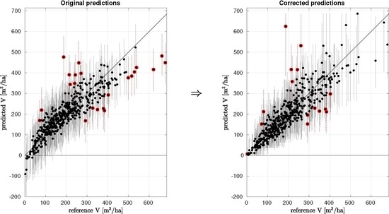
Common statistics used to evaluate the performance of the method may show relatively good behaviour for the predictions: the mean difference (MD) can be close to zero and the root mean square error (RMSE) sufficiently small. However, the overall variance of the predicted attribute values can be smaller than that of the reference set. The lack of model fit generally causes problems especially with the largest and smallest values of the attribute, see Figure 1 for an example of linear model-based point predictions and their 95% probability intervals of forest attribute total volume (V [m${}^3$/ha]) in study site Loppi–Janakkala, which is one of the cases validated later in this study. Here, the prediction errors are most likely a result of lack of correlation between remotely sensed data and the attribute field measurements which can be partly caused by errors in used data.

The large attribute values (>400 ${\mathrm{m}}^3/\mathrm{ha}$) are systematically under-estimated and also the small attribute values (<50 ${\mathrm{m}}^3/\mathrm{ha}$) are under-estimated. Here, the smallest, close to zero attribute values are even predicted to be negative, which is an unwanted property of linear models. The same properties of the predictions can be seen also in the accuracy assessment linear fit, also known as the geometric mean functional relationship (GMFR), between attribute reference set (the field measurements) and attribute point predictions. Here, the slope of the red linear fit line is less than one. In an optimal case, the red linear fit line would have slope one (parallel with the 1-1 line), and intercept value equal to the mean value of the attribute reference set.

Figure 1b shows a typical case of linear model-based probability intervals, which in this case follow a normal distribution defined by the model formulation [13]. In many linear and non-linear models the prediction distributions are assumed to be normally distributed, thus such a case is used as an example here. In this set of predictions, 95% of the reference attribute values were within the estimated 95% probability intervals of corresponding predictions, but the largest attribute values of the reference set tended to be systematically underestimated and also outside the probability interval, see red point predictions and probability intervals in Figure 1b. In an ideal case the 5% of the attribute reference set values outside the probability interval should be relatively uniformly distributed along the reference set attribute distribution and include both too small and too large predictions.

Excessive averaging and systematic under- or over-estimation—and even more the outright qualitative prediction errors like negative values—have many unwanted consequences. For example, in AGB prediction in incorporating carbon captured into tropical forest in climate financing schemes like UN REDD+ [14,15,16], the plots with LiDAR data-based AGB predictions can be used as surrogate plots in larger area AGB predictions based on satellite data. If the variance of surrogate AGB prediction distribution is under-estimated, the problem is amplified in the final, larger area predictions. Also, if the distribution scatter-grams are rendered flat by saturation for the largest AGB values, then any gains in carbon capture are heavily damped by the statistics used in assessing them. The lack of fit and under-estimation of large values can be accumulated to other levels of prediction also, such as stand level predictions or large plot/grid cell predictions. If the forest is divided into stands according to the homogeneity of the forest, it is likely that plot level attribute values of similar magnitude are located in the same stand and the stand level prediction composed of a (weighted) average of predicted attribute values in plots inside the stand will suffer from the same problems as plot level predictions.

It is a common procedure to use a suitable post-processing or transformation method to overcome this type of problems, see e.g., [17,18,19,20,21]. Statistical post-processing methods like histogram matching or quantile–quantile mapping transformation utilize the shape of the underlying attribute training set distribution to correct new attribute predictions. The attribute training set data distribution shapes can be estimated with parametrized, fixed shape distribution functions or arbitrary, non-parametric distribution functions.

Histogram matching algorithms are commonly used to process satellite data [19,22], and quantile–quantile mapping transformations are used for bias correction of regional climate models [18,23]. It has shown its power also in correction of forest attribute predictions given by k-NN method, see [20] for a parametric approach and [21] for a nonparametric approach. In the forest inventory application, the non-parametric approach which is based on arbitrary shapes of attribute distribution is a natural approach especially if we wish to have a method that generalizes well to any forest attribute of interest in any study site. In regional climate models, a study of [23] showed that nonparametric transformations had the highest skill in systematically reducing biases in precipitation. Statistical transformations assume that the modelled relation holds also with new data, thus the attribute distribution data used as the training set must be a proper probability sample of the whole population.

The aim of this study is to develop a non-parametric quantile–quantile mapping transformation based on empirical quantiles (QUANT) used e.g., in [18,21,23] for operational, plot level forest inventory for both attribute point predictions and, as a novel approach, uncertainty analysis of the predictions.

As an example case, we validate the performance of the QUANT post-processing method using a linear model with LiDAR data based predictors to generate the raw predictions. The post-processing procedure would be similar for raw predictions estimated with any other method once they are based on a training set, i.e., we have a sample of the real underlying distribution of the forest attribute of interest. In this study we expand our transformation to the natural property of the linear model, the prediction probability interval, as well. The proposed uncertainty analysis can also be adapted to predictions of other models as well, as long as the model generates prediction distributions for the raw predictions.

The performance of the post-processing method is validated both visually and numerically using real forest inventory data with large training set sizes (over 400 field plots) and the robustness of the proposed method is validated also for a reduced number of training set plots. Because of the challenges linked to a small training set size combined with multidimensional, correlated predictors, we use a formulation of the linear model which has shown to be efficient in such situations, the Bayesian Principal Component Regression model (BPCR) introduced in [13].

This article is organized as follows: In Section 2, the details of the proposed method, the remotely sensed data, the field data, the validation procedure, and the parameters that are used as indicators of method performance are introduced. In Section 3, results for different test cases are given. The results are discussed in Section 4 and then the conclusions about the performance and the pros and cons of the proposed post-processing method are given in Section 5.

2. Materials and Methods

The forest inventory attribute of interest, given as a vector $\mathit{y}$, is assumed to have real, non-negative values. In the area based approach, the forest attribute is predicted at a plot or grid cell level with a suitable model. A training set of size n (plots) is used to estimate the model parameters. The training set contains field measurements of the forest attribute, ${\mathit{y}}_t$, and the remotely sensed data-based predictors, ${\mathit{X}}_t$, for each plot in the training set t. The attribute values are predicted in the validation set v that consists of new plots or grid cells using the set of predictors ${\mathit{X}}_v$.

Here we use a linear model-based approach that uses singular value decomposition of predictors and automatically emphasizes the use of those singular vectors that best explain the data, BPCR, to estimate the model parameters [13]. The method is well suited for the cases with highly multicollinear predictors, as if often the case with LiDAR predictors, and small number of field sample plots.

Each new, individual plot/grid cell level prediction ${\tilde{\mathit{y}}}_i$ given by the used linear model follows the normal distribution with estimated mean value ${\mu }_i$ and variance ${\sigma }_i^2$, ${\tilde{y}}_i\sim N({\mu }_i,{\sigma }_i^2)$. In general, the point prediction for the plot is given as the expected value of the normal distribution, ${\mu }_{{\tilde{y}}_i}$, and $(1-\alpha )$% prediction probability interval is given as $(\alpha /2,1-\alpha /2)$-quantiles of the symmetric normal distribution.

2.1. Non-Parametric Quantile–quantile Mapping Transformation

In the QUANT post-processing method, the training set distribution of the attribute is treated as the true distribution of the forest attribute values in the given area, and compared to the corresponding distribution of the predictions in the training set plots. The distributions are represented by the empirical cumulative distribution functions (ECDFs) where the distribution of a sample (given as an ordered set from smallest to largest value) is represented as a cumulative function

$${\widehat{F}}_{\mathit{y}}\left(y_j\right)=n^{-1}\left(\sum _{k=1}^{n}I(y_k\le y_j)-\frac{1}{2}\right),j=1,2,\dots ,n,$$

(1)

where $I(y_k\le y_j)$ is the indicator function which is equal to one if $y_k\le y_j$, and zero otherwise. The values of ${\widehat{F}}_{\mathit{y}}\left(y_j\right)$ vary between zero and one, scaled such that ${\widehat{F}}_{\mathit{y}}\left(y_j\right)$ gets values $\frac{1}{n}\left\{\frac{1}{2},1+\frac{1}{2},2+\frac{1}{2},\dots ,n-\frac{1}{2}\right\}$. The ECDF values between the measurements are estimated as a piece-wise linear interpolation.

When using linear model-based raw predictions, some values of the raw predictions in new plots may exceed the extreme values found in the training set raw predictions. In such a case, simple extrapolation similar to [18] is used: outside the range of training set values, the same slope as between the last two extreme points in the data is kept. For instance, the piece-wise linear interpolation curve between the first two ordered points $(y_1,y_2)$ with corresponding to ECDF values $(\frac{1}{2n},\left(1+\frac{1}{2}\right)\frac{1}{n})$, holds also for the ECDF range $(0,\frac{1}{2n})$, and similarly to to the upper tail of the ECDF.

The ECDF values for the training set field measurements of the attribute, ${\mathit{y}}_t$, and for the raw predictions of the training set, ${\tilde{\mathit{y}}}_t$, are constructed separately using Equation (1), resulting to ECDFs ${\widehat{F}}_{{\mathit{y}}_t}\left(\right)$ and ${\widehat{F}}_{{\tilde{\mathit{y}}}_t}\left(\right)$, correspondingly. Figure 2a illustrates the ECDFs of certain values in training set predictions, ${\tilde{\mathit{y}}}_t$ (which in this case correspond to the mean values of the prediction distributions, ${\mu }_t$), and corresponding training set field measurements, ${\mathit{y}}_t$, of the case shown in Figure 1.

The quantile–quantile mapping technique QUANT corrects the raw predictions according to their ECDF values among the training set predictions. The cumulative distribution function value $P={\widehat{F}}_{{\tilde{\mathit{y}}}_t}\left({\tilde{\mathit{y}}}_i\right)$ of the prediction ${\tilde{\mathit{y}}}_i$ in new plot i is transformed such that the value, ${\tilde{\mathit{y}}}_{i,\mathrm{corr}}$, that gives the same ECDF value among the training set field measurements ${\mathit{y}}_t$, is found, i.e., ${\widehat{F}}_{{\mathit{y}}_t}\left({\tilde{\mathit{y}}}_{i,\mathrm{corr}}\right)=P$. The transformation model $T_{{\mathit{y}}_t,{\tilde{\mathit{y}}}_t}\left({\tilde{\mathit{y}}}_i\right)$ to transform ${\tilde{\mathit{y}}}_i$ from training set prediction distribution to training set field measurement distribution is given by

$${\tilde{\mathit{y}}}_{i,\mathrm{corr}}=T_{{\mathit{y}}_t,{\tilde{\mathit{y}}}_t}\left({\tilde{\mathit{y}}}_i\right)={\widehat{F}}_{{\mathit{y}}_t}^{-1}\left({\widehat{F}}_{{\tilde{\mathit{y}}}_t}\left({\tilde{\mathit{y}}}_i\right)\right).$$

(2)

In the transformation model, similar extrapolation is applied also to the smallest values which might be smaller than the first quantile of the training set predictions. However, only non-negative values are accepted for the training set field measurement ECDF, as the real attribute values are always non-negative, and thus the ECDF (and probability) of such points is set to zero. See the Figure 2b for the transformation function corresponding to the distributions in Figure 2a.

2.2. Uncertainty Analysis for the Transformation

Plot level predictions given by models with possibly imperfect model fit and parameter distributions estimated using a limited number of field measurements, include uncertainty. Linear model-based plot level predictions, for instance, include this information of uncertainty as a normal distribution with estimated variance around the mean value (point prediction), which is used as the “predicted value”. Thus, each new plot level prediction is given as a normal distribution.

In our post-processing procedure, the uncertainty for a new plot $v_i$ in the validation set can be included by sampling from the attribute prediction distribution of the plot, ${\tilde{y}}_{v_i,m}\sim N({\mu }_{v_i},{\sigma }_{v_i}^2)$, $m=1,2,\dots ,n_{\mathrm{sim},v}$, and then using the transformation function, Equation (2), for all the sampled prediction distribution points. However, because of uncertainty in linear model-based predictions, there is also uncertainty among the plot level predictions in the training set, which causes uncertainty also in the transformation function. Thus, also the training set plot level predictions are sampled, ${\tilde{\mathit{y}}}_{t,l}\sim N({\mu }_t,{\sigma }_t^2),l=1,2,\dots ,n_{\mathrm{sim},t}$, and the resulting ECDF function (1), ${\widehat{F}}_{{\tilde{\mathit{y}}}_{t,l}}\left(y\right)$, is used to generate the new transformation function $T_l\left(y\right)=T_{{\mathit{y}}_t,{\tilde{\mathit{y}}}_{t,l}}\left(y\right)$ for each sample set l. Thus the transformation of the prediction distribution points is performed by sampling from the training set predictions which are then used to generate the transformation of the sampled prediction distribution points.

In Figure 3, the transformation procedure is illustrated for one example plot. The normal distribution of the raw prediction for a new plot, represented here as a sample generated from the given plot level prediction distribution, is transformed using the samples of predicted training set plots. The transformed distribution is no longer normal, but has an arbitrary shape. Also, the transformation curve is not symmetric around the mean value transformation curve, $T_{{\mathit{y}}_t,{\tilde{\mathit{y}}}_t}\left(\right)$. This is caused by the ECDFs of training set prediction samples, where the spread of predictions is larger than with the mean value predictions, which cause the sampled transformation curves to have a larger spread on x-axis (original, raw predictions).

The asymmetry and arbitrariness of the transformed new plot prediction sample must be taken into account when estimating the probability interval. By definition, for example, the 95% ($\alpha =0.05$) probability interval is estimated by finding $[a,b]$ such that

$$\mathrm{Pr}(a\le y\le b)=0.95.$$

(3)

Here, Pr is the probability, which can be estimated using the sample point distribution. That is, 95% of the sample points must be within the given interval, which is obviously not a unique interval. In this paper, the narrowest interval that satisfies the condition (3) is chosen, similar to [24], and we require also that the transformed mean value of the validation plot distribution is within the given probability interval.

Although the transformed mean value of the validation plot distribution is no longer at the mean, mode nor the median of the transformed probability distribution, it presents the corrected prediction because it is estimated with the best information we have: the most likely value of the raw predictions (the mean and the mode of the normal distribution), transformed with the most likely training set prediction values (the mean values).

The whole algorithm is given as:

• Estimate model parameters and corresponding model with training data ${\mathit{y}}_t,{\mathit{X}}_t$.
• For each validation set plot $v_i$:

  (a)

  Estimate the prediction probability distribution with the given model. Estimate the point prediction as the mean value ${\tilde{y}}_{v_i}={\mu }_{v_i}$.

  (b)

  Generate the post-corrected prediction ${\tilde{y}}_{v_i,\mathrm{corr}}=T_{{\mathit{y}}_t,{\tilde{\mathit{y}}}_t}\left({\tilde{y}}_{v_i}\right)$ using ${\tilde{\mathit{y}}}_t={\mathit{\mu }}_t$.

  (c)

  Generate the sample of $n_{\mathrm{sim},v}$ prediction distribution points ${\tilde{\mathit{y}}}_{v_i,m}\sim N({\mu }_{v_i},{\sigma }_{v_i}^2)$, $m=1,2,\dots ,n_{\mathrm{sim},v}$ (here $n_{\mathrm{sim},v}=1000$).

  (d)

  For $l=1,2,\dots ,n_{\mathrm{sim},t}$ (here $n_{\mathrm{sim},t}=100$)

  (i)

  Generate a new sample of n training set predictions ${\tilde{\mathit{y}}}_{t,l}\sim N({\mathit{\mu }}_t,{\sigma }_t^2)$.

  (ii)

  Generate ECDF function ${\widehat{F}}_{{\tilde{\mathit{y}}}_{t,l}}\left(y\right)$ and the corresponding transformation function $T_l\left(y\right)=T_{{\mathit{y}}_t,{\tilde{\mathit{y}}}_{t,l}}\left(y\right)$.

  (iii)

  Transform all prediction distribution points: ${\tilde{\mathit{y}}}_{v_i,m,l,\mathrm{corr}}=T_l\left({\tilde{\mathit{y}}}_{v_i,m}\right)$.

  (e)

  Use the $n_{\mathrm{sim},v}·n_{\mathrm{sim},t}$ transformed prediction distribution points to analyze the $(1-\alpha )\%$ probability intervals as described above.

2.3. Study Sites

In this study, forest inventory data from seven separate study sites in different parts of Finland are used to evaluate model performance and to validate the consistency of the results. The sites are located at Matalansalo (Heinävesi), Juuka, Loppi–Janakkala, Pello, Lieksa, Kuhmo, and Karttula. For more detailed information of the datasets used, see [25]. A total of 472, 511, 441, 553, 483, 470, and 538 field plots were measured in each study site, respectively. These study sites belong to the boreal forest type comprising mostly species like Scots pine (Pinus sylvestris), Norway spruce (Picea abies), and different species of hardwoods, mostly birch.

2.3.1. Field Measurements

The sample plots of the study sites were selected with a number of different sampling strategies. Some sites were equipped with a regular sample plot grid, some others were equipped with regularly sampled plot clusters, and still others were equipped with randomly selected plots. Sample plots were always circular plots with a 9-m radius. They were positioned at first with a hand-held global positioning systems (GPS), and the exact position of the plot center was later calculated during measurement and differentially corrected offline.

In this article, we used field measurements of three forest attributes: median tree height (Hgm, [m]), total volume (V, [m${}^3$/ha]), and stem number (SN, [number of stems/ha]). They were estimated from the field measurements in a similar manner at each site, using models of Veltheim [26].

2.3.2. Remotely Sensed Data

The auxiliary data covering the whole study site areas consist of LiDAR measurements and aerial images from each study site, except in Matalansalo where only LiDAR measurements were available.

LiDAR scanning of the different areas was conducted from 2004 until 2008. Three different types of scanners were used, namely Optech ALTM 3600, Leica ALS50, and Leica ALS60. Flying height varied between 700 m and 2000 m, and scanner pulse frequency varied between 58,900 Hz and 125,100 Hz. LiDAR data were clipped to plot extent before LiDAR predictors were extracted. A set of 38 candidate predictors were derived from LiDAR measurements for each sample plot used. This set is similar to the set that has been used in [27]. It consists of percentile points and cumulative percentile parts of the first and last pulse heights of non-ground hits (height $>2$ m), percentile intensities of first and last pulse intensities of non-ground hits, mean of first pulse heights $>5$ m, standard deviation of first pulse height, and the number of measurements $<2$ m of first and last pulse heights divided by the total number of the same measurements of each plot, depicting vegetation density.

The digital aerial photographs consist of pixel sizes of 0.5 m and three or four channels. Digital ortho-rectified aerial images were used with 0.5 m spatial resolution. The channels used were in most cases blue, green, red and near-infrared. Two candidate predictors, namely percentage of hardwoods and percentage of conifers, were visually interpreted from these images using the approximately 1000 pixels in each plot: The pixels were classified as hardwood trees, conifer trees and hits to the ground, and the resulting candidate predictors were the percentages of hardwood trees (Hwd) and conifer trees (Cnf) in each plot.

As a result, a total of 38 candidate predictors were available for study site Matalansalo and 40 candidate predictors for the other study sites. These predictors were highly correlated with each other with condition numbers between 6400 and 25,350 among different study sites, which means severe multicollinearity.

2.4. Validation Procedure

Leave-One-Plot-Out (LOPO) cross-validation procedure is used to validate the performance of the proposed method. In LOPO, from the total of N plots available, one plot at time is chosen into the validation set, and the rest $N-1$ plots serve as training set plots. The parameters of the linear model used to generate the raw predictions are estimated with the training set data chosen (predictors and measured attribute values of the training set plots), and the attribute prediction distribution of the validation plot is estimated using the resulting model with the validation set predictor values. The post-processing method uses the predicted training set distributions and the training set field measurement values of the attribute to transform the raw validation plot point prediction and its probability distribution. This procedure results in a vector of N point predictions for both raw predictions, $\tilde{\mathit{y}}$, and corrected predictions, ${\tilde{\mathit{y}}}_{\mathrm{corr}}$, with corresponding probability intervals.

If a reduced number of training set plots is used, the training set plots are selected randomly from the $(N-1)$ leave-one-out plots. This selection method is assumed to give proper, representative samples. Thus, $n<N$ plots are selected from the $N-1$ plots available in each LOPO repetition.

2.5. Model Performance Estimates

Performance of the QUANT post-processing method is compared to the performance of the BPCR method, i.e., we compare the quality of the post-processed predictions to the quality of the raw predictions.

The first validation parameter is the relative mean difference between the predictions and corresponding reference values,

$$\mathrm{D}\%=\frac{{\sum }_{i=0}^N\left({\tilde{\mathit{y}}}_i-{\mathit{y}}_i\right)}{N}\times \frac{100(\%)}{\overline{\mathit{y}}},$$

(4)

where $\tilde{\mathit{y}}$ is a vector of the point predictions (either raw predictions or post-corrected predictions), $\mathit{y}$ is the corresponding attribute values in the reference set, and $\overline{\mathit{y}}$ is the average of the reference set values. The hypothesis of whether the mean difference deviance from zero is significant, is tested by one sample mean t-test and deviances with p-values less than the given significance level $\alpha =0.05$ are considered significant.

The second validation parameter is the relative root mean square error,

$$\mathrm{RMSE}\%=\sqrt{\frac{{\sum }_{i=0}^N{\left({\tilde{\mathit{y}}}_i-{\mathit{y}}_i\right)}^2}{N}}\times \frac{100(\%)}{\overline{\mathit{y}}},$$

(5)

which describes the standard deviation of the prediction residuals.

A validation parameter describing the linear relationship between the reference values and the point predictions uses a linear model with the intercept and the reference vector as predictors and the vector of predictions as the response. The linear model parameters $c_0$ and $c_1$ for the intercept and the reference values are estimated. For perfect predictions, the intercept parameter $c_0$ is equal to the reference mean and the slope $c_1$ is one. In practice, the difference between $c_0$ and $\overline{y}$ is equal to mean difference, $\mathrm{D}$. Thus, only $c_1$ is shown in this study.

We also validate the relative mean absolute error of the differences between the P:th quantiles in the attribute point prediction distribution and the reference distribution, MAE%. Quantiles $\mathit{p}=\{0.00,0.05,\dots ,0.95,1.00\}$ are used. For perfect point predictions, MAE% is zero.

The probability intervals of each prediction distribution are also estimated. Here, the fraction of reference set values that fall in the 95% percent probability interval of the corresponding prediction distribution are calculated ($\mathrm{P}95$), and with the 95% probability interval, this fraction should be approximately 95%. Also, the average of the probability interval widths over the whole validation set predictions is calculated (${\mathrm{PI}}_{\mathrm{ave}}$).

3. Results

3.1. Large Training Set Size Results

Prediction error statistics for the forest attributes Hgm, V and SN are given in

Table 1. Plot level LOPO results for all the study sites and forest attributes. The relative changes in the RMSE%, slope error $|1-c_1|$ and MAE% after the post-processing with QUANT method are shown in brackets.

Hgm	Method	RMSE	RMSE%	D%	$|1-{\mathit{c}}_1|$	MAE%	${\mathbf{PI}}_{\mathbf{ave}}$	${\mathit{P}}_{95}$
Matalansalo	BPCR	1.48	8.71	−0.01	0.08	1.72	5.79	94.07
	QUANT	1.53	8.99 (3.2%)	−0.02	0.04 (−48.4%)	0.23 (−86.8%)	5.72	94.92
Juuka	BPCR	1.38	9.43	0.00	0.14	1.96	5.39	95.50
	QUANT	1.42	9.69 (2.8%)	0.02	0.07 (−48.7%)	0.22 (−88.7%)	5.34	95.30
Loppi−Janakkala	BPCR	1.93	11.06	−0.01	0.13	2.03	7.52	94.33
	QUANT	1.99	11.38 (3.0%)	−0.02	0.07 (−48.1%)	0.48 (−76.4%)	7.39	94.33
Pello	BPCR	1.15	9.83	0.02	0.19	2.96	4.47	94.21
	QUANT	1.21	10.33 (5.1%)	0.03	0.10 (−48.4%)	0.72 (−75.6%)	4.49	94.21
Lieksa	BPCR	1.43	9.03	0.00	0.08	1.94	5.61	94.82
	QUANT	1.48	9.35 (3.6%)	−0.04	0.04 (−43.5%)	1.08 (−44.5%)	5.49	94.62
Kuhmo	BPCR	1.32	8.37	0.01	0.27	2.15	5.15	95.74
	QUANT	1.38	8.77 (4.8%)	0.01	0.14 (−47.1%)	0.46 (−78.5%)	5.12	95.32
Karttula	BPCR	1.60	9.03	0.01	0.09	2.04	6.25	93.68
	QUANT	1.62	9.12 (1.0%)	0.02	0.04 (−51.8%)	0.22 (−89.3%)	6.14	93.49
V
Matalansalo	BPCR	40.43	19.88	−0.03	0.15	8.87	157.58	94.07
	QUANT	42.46	20.88 (5.0%)	0.12	0.08 (−47.8%)	1.98 (−77.7%)	152.14	95.97
Juuka	BPCR	26.44	18.18	0.00	0.10	3.00	102.67	92.76
	QUANT	27.44	18.86 (3.8%)	0.05	0.06 (−47.2%)	1.40 (−53.2%)	97.55	92.95
Loppi–Janakkala	BPCR	53.37	26.26	−0.08	0.21	10.69	206.17	95.01
	QUANT	56.23	27.67 (5.4%)	0.11	0.11 (−47.0%)	0.70 (−93.4%)	196.07	96.60
Pello	BPCR	26.09	25.38	0.02	0.22	8.17	100.76	93.67
	QUANT	26.79	26.07 (2.7%)	−0.09	0.12 (−44.2%)	0.60 (−92.7%)	95.83	93.13
Lieksa	BPCR	52.04	26.71	0.03	0.16	10.61	202.96	92.96
	QUANT	57.28	29.40 (10.1%)	0.31	0.09 (−46.3%)	1.39 (−86.9%)	188.08	94.62
Kuhmo	BPCR	48.48	24.82	0.02	0.28	8.15	188.25	93.62
	QUANT	50.45	25.83 (4.1%)	0.08	0.15 (−45.7%)	1.61 (−80.2%)	179.25	93.62
Karttula	BPCR	54.37	26.41	−0.08	0.19	11.29	210.48	94.61
	QUANT	53.41	25.94 (−1.8%)	−0.08	0.10 (−47.5%)	1.53 (−86.4%)	188.86	95.54
StemNo
Matalansalo	BPCR	409.57	27.18	−0.09	0.35	9.04	1600.67	93.43
	QUANT	428.56	28.44 (4.6%)	−0.03	0.19 (−45.7%)	1.18 (−86.9%)	1501.50	94.28
Juuka	BPCR	370.39	28.83	−0.01	0.40	12.81	1450.98	93.93
	QUANT	389.68	30.33 (5.2%)	0.14	0.22 (−44.8%)	1.92 (−85.0%)	1364.73	93.74
Loppi–Janakkala	BPCR	423.69	38.21	−0.03	0.42	14.97	1647.06	95.24
	QUANT	467.26	42.13 (10.3%)	0.03	0.26 (−39.5%)	1.51 (−89.9%)	1477.50	94.56
Pello	BPCR	730.64	55.14	−0.09	0.65	27.70	2877.51	96.02
	QUANT	831.57	62.75 (13.8%)	0.04	0.42 (−35.4%)	1.39 (−95.0%)	2513.21	95.12
Lieksa	BPCR	367.16	30.98	−0.00	0.42	13.29	1433.14	94.62
	QUANT	408.99	34.51 (11.4%)	0.13	0.25 (−40.3%)	1.68 (−87.4%)	1337.33	94.82
Kuhmo	BPCR	331.15	32.99	−0.04	0.46	15.14	1290.36	94.89
	QUANT	369.87	36.85 (11.7%)	0.25	0.27 (−42.7%)	2.68 (−82.3%)	1226.67	96.81
Karttula	BPCR	473.65	41.16	−0.11	0.49	26.09	1843.31	95.72
	QUANT	579.19	50.34 (22.3%)	0.47	0.32 (−35.9%)	6.79 (−74.0%)	1635.42	96.47

. The results show that the optimal RMSE (and RMSE%) values are achieved by the raw, linear model-based predictions (BPCR) for each attribute in each site, while the RMSE of post-processed predictions (QUANT) is slightly larger in each case. The RMSE% for predictions of Hgm is 1.0–5.1% (3.4% on average) larger for post-processed predictions than for the raw predictions, depending on the study site. For attribute V the deterioration is −1.8–10.1% (4.2%) and for SN 4.6–22.3% (11.3%). On the average, RMSE% is deteriorated 6.3% among different attribute values in different study sites.

The attribute Hgm represents here the attributes that are predicted with small RMSE% and good fit even with the linear model only. Thus, there is not much to improve in the results. Attribute V represents a typical attribute for which small problems with the low precision and model fit that need improvement occur. Attribute SN represents the most challenging case, for which the precision is quite low and the model fit is poor giving under-estimation for large values of the attribute.

For each attribute in each site, the mean difference, D%, of the predictions doesn’t deviate significantly from zero. The linear model fit, on the other hand, is better for the QUANT method in terms of the slope, $c_1$: In each case, the slope is closer to one ($|1-c_1|$ closer to zero) than for the BPCR model. The improvement is 43.5–51.8% for attribute Hgm, 44.2–47.8% for V and 35.4–45.7% for SN. Also the parameter that describes the distribution of the predicted values compared to the true distribution of the reference set, MAE%, is always substantially smaller for QUANT method than for BPCR model. For the attribute Hgm the improvement is 44.5–89.3%, for V 53.2–93.4% and for SN 74.0–95.0%.

There are two cases where the MAE% is not improving as much as in the other cases: Juuka attribute V and Lieksa attribute Hgm. The raw prediction (BPCR) MAE% for attribute V in study site Juuka is very good, 3.00%, compared to the other study sites with over 8% MAE%, and thus the post-processing method that results in similar scale QUANT MAE% in Juuka as in other study sites, shows less improvement. Also the improvement of MAE% for attribute Hgm in Lieksa, 44.5%, is smaller than for the other study sites with over 75% improvement. Although QUANT method corrects the Hgm prediction distribution close to zero quantile differences from the reference set distribution, the largest Hgm value of the reference set distribution is not corrected as much, and thus the mean absolute error of quantiles remains larger after correction. In Lieksa, ECDF of the Hgm reference set distribution grows rapidly until the second largest value of measured Hgm, after which the growth is much slower to the largest measurement. Thus, when there is no measurement for the largest value included in the training set, the training set sample does not represent the whole population and the extrapolated ECDF tail does not include the extreme values, see Figure 4.

Results for the attribute plot level prediction uncertainties are reasonable good for both methods. The fractions of plots for which the truth is within the estimated 95% probability interval, is roughly 95% for all the cases. Thus, the estimated probability interval widths are wide enough to cover the real uncertainty, but on the other hand, not too wide. The probability interval widths for both methods are on the average quite similar. For attributes V and SN, the average probability intervals of the proposed method, QUANT, are slightly narrower, meaning less uncertainty for the plot level predictions on the average. This could be partly explained by removing of the negative values from the transformed probability intervals.

As an example of the corrected point predictions and the corresponding probability intervals, see Figure 5 for the case of attribute V in study site Loppi–Janakkala. As seen in Table 1, the RMSE% and D% of the corrected predictions in this case are nearly equal to those of the raw predictions. The distribution of the corrected predictions follow much better the distribution of the attribute field measurements, the truth (MAE% close to zero and $c_1$ close to one), which can be also seen in Figure 5a. Within this sample, 97.3% of the true attribute values were within the given probability intervals of corrected predictions, and those points that were outside this interval were distributed more uniformly along the distribution of the attribute reference values, see Figure 5b. The probability intervals show heteroscedastic behaviour, i.e., the interval is smaller for small attribute values, and increases for larger values. Almost all large attribute reference values are within the corrected probability intervals, unlike in the case of raw predictions, where the largest attribute reference values were systematically outside the given probability intervals, compare to Figure 1. Examples of cases with only little correction effect (attribute Hgm) and large correction effect (attribute SN) are shown in Figure 6, Figure 7 and Figure 8.

In the case of Hgm, the precision of the original, raw predictions is good and they correlate well with the reference set attribute values, and thus the transformation function does not include much transformation, see Figure 6a. This can be seen also in the raw and corrected predictions accompanied with the probability intervals, see Figure 7, where not much change occurs. On the contrary, the transformation function of attribute SN causes larger changes in the point predictions and probability intervals. Especially for the large values of raw predictions, the transformation function has a large effect and also the uncertainty increases, see Figure 6b. Figure 8 shows that the largest values are systematically under-estimated among the raw predictions such that the reference set attribute values are not even within the probability intervals and the linear model is unable to predict those values. After correction, the uncertainty of these values is better registered, as the wider probability intervals and transformed predictions cover a higher percentage of these plots. However, even the corrected predictions do not manage to completely overcome the under-estimation of the largest values. On the other hand, the small values of SN are well covered with the narrower probability intervals of the corrected predictions. In practice, these two cases represent the two extremes of typical transformations and the resulting behaviour of corrected point predictions and probability intervals.

3.2. Reduced Training Set Size Results

Figure 9 shows the estimated validation statistics as a function of reduced training set size in the example study site Loppi–Janakkala. In the tests, the behaviour of error statistics was similar in all the study sites, thus here we show results of only one study site.

Overall, the results remain close to the baseline results, i.e., the attribute predictions estimated with a large training set size, even with training set sizes as small as 100–150 plots depending on the attribute of interest. As seen in the the sub-figures, the relative difference RMSE%, slope $c_1$ error, MAE% and ${\mathrm{PI}}_{\mathrm{ave}}$ between the raw predictions and the post-processed predictions remain similar as in Table 1 for all the training set sizes. The mean difference of the predictions, D%, did not differ significantly (this was validated with t-tests using $\alpha =0.05$) from zero for any of the attributes at any site and training set size. Also the coverage of the probability intervals, $P_{95}$ shows to be consistent.

4. Discussion

In general, the largest interest in operational forest inventory campaigns in boreal forests in Nordic countries and Canada lies in the largest trees which are most valuable for timber use, or in case of carbon credits in tropical forests, hold the most carbon. As discussed in this article and references given, the commonly used remotely sensed data-based prediction methods tend to under-estimate the height and volume in plots containing such trees. The results given here show that the QUANT post-processing method gives reliable and accurate predictions for plots within forest that contains tall trees and a large timber volume and covers the uncertainty connected to such cases better than the raw predictions. Although the RMSE% values of the post-processed predictions tend to be larger than those of the raw predictions, the difference is relatively small, which supports the results given in [21]. The gain in the preservation of the attribute distribution characteristics and range combined with the better model fit without under- or over-estimation of values in any range can be considered more important than the small reduction in the average prediction precision. The proposed method is applicaple to different models using different predictor data sources and predicting different attributes as its performance depends only on the quality of the raw attribute predictions compared to the training set attribute measurements. In case of e.g., tropical forest biomass estimation, the precision of the raw predictions based on LiDAR data generally tends to be of similar scale and form as those of the stem number predictions studied here. In our unpublished study, we found that for linear method based predictions of above ground biomass in Nepal (see [16] for more information about the data) the RMSE% increased 8.6%, the slope error decreased 42.5% and the MAE% decreased 86.4% and the uncertainty estimation gave correct probability intervals with slightly decreased interval widths. These relations held with training set sizes between 50–737 plots, and the results remained close to optimal for training set sizes as small as 100–150. These results align well with the results shown above for other forest types.

The QUANT post-processing method did not introduce any significant, additive deviation from zero in the mean difference of the predictions. This is reasonable as the post-processing fits the transformed attribute prediction distribution to the attribute distribution of the training set. If the training set is a proper, representative probability sample of the whole population, also the predictions fitted to that sample should, having approximately the same mean value, have zero mean difference compared to the truth.

Important property of the prediction methods, the ability to estimate the plot level $(1-\alpha )$% probability interval together with the point estimate, is retained in the post-processing procedure. The post-processed probability intervals appear to be more reasonable than those of the of the raw predictions generated by e.g., a linear model, for which the interval shows behaviour of a homoscedastic variance. The probability intervals of the raw attribute predictions tend to be too wide for the near zero values of the attribute, while they can easily be under-estimated for large values of the attribute. The post-processed probability intervals tend to be smaller for small attribute values and larger for the large attribute values.

The proposed post-processing method shows to be robust against reduction in the training set size, i.e., number of used field plots. The performance of the QUANT method depends on the performance of the prediction method used for the raw predictions, and the relation between the raw and post-processed prediction results remains similar for all the training set sizes tested.

The correlation between attributes is not incorporated into the proposed post-processing method. However, as shown in Figure 10, the post-prosessing of the raw predictions is not violating the correlation structure of the attributes much in our test case, but since this property is not included intrinsically in the proposed method, one must be careful with the impossible or unacceptable correlations among the predictions.

5. Conclusions

The results of this study show that the proposed post-processing method, QUANT, can be used to correct the statistical defects in the predictions generated with some common remotely sensed data-based methods used in forest inventory. Here, the raw predictions were estimated with a linear model, but the method could be applied to other approaches as it uses only the attribute field measurements available and compares them to their predictions. For uncertainty analysis, the uncertainty of the raw predictions must be estimated. The post-processing method produces predictions from the whole range of the true distribution of the attribute values and corrects the skewness in the distribution so that within any range of attribute values, there is no systematic over- or under-estimation. The precision of the post-processed predictions can be slightly worse than the precision of the raw predictions.

The proposed post-processing procedure is based only on the distribution of the attribute values in the selected training set plots. No assumptions on the shape of the attribute distributions are needed since the method is based only on the empirical cumulative distribution function of the available field sample of the attribute. The method is general; it can be used to any shape of distributions and for any attribute of interest, as long as a proper, representative probability sample of the attribute values exists.

In this study only a random training set plot selection procedure was tested in order to validate the effect of reduction of the training set size. The formulation of QUANT method makes it sensitive to defects in the field sample, i.e., training set, selection. If the training set is not a proper, representative probability sample of the true population in the study site, it will probably effect also the post-processing procedure such that the mean difference of predictions can deviate significantly from zero. Thus, when using this method, special care should be given to training set quality and the field plot selection criteria.

Different forest attribute values were predicted as individual, separate outputs in this study. In the real world, there is a correlation among different attributes, even some rules, such as in case of species-specific attributes for which the corresponding total attribute is a sum of the species-specific values. In future research, the post-processing method should be extended to use and preserve also the correlation structures of the attributes of interest.