Wavelet-Based Correlation Identification of Scales and Locations between Landscape Patterns and Topography in Urban-Rural Profiles: Case of the Jilin City, China

Abstract

Landscapes display overlapping sets of correlations in different regions at different spatial scales, and these correlations can be delineated by pattern analysis. This study identified the correlations between landscape pattern and topography at various scales and locations in urban-rural profiles from Jilin City, China, using Pearson correlation analysis and wavelet method. Two profiles, 30 km (A) and 35 km (B) in length with 0.1-km sampling intervals, were selected. The results indicated that profile A was more sensitive to the characterization of the land use pattern as influenced by topography due to its more varied terrain, and three scales (small, medium, and large) could be defined based on the variation in the standard deviation of the wavelet coherency in profile A. Correlations between landscape metrics and elevation were similar at large scales (over 8 km), while complex correlations were discovered at other scale intervals. The medium scale of cohesion and Shannon’s diversity index was 1–8 km, while those of perimeter-area fractal dimension and edge density index were 1.5–8 km and 2–8 km, respectively. At small scales, the correlations were weak as a whole and scattered due to the micro-topography and landform elements, such as valleys and hillsides. At medium scales, the correlations were most affected by local topography, and the land use pattern was significantly correlated with topography at several locations. At large spatial scales, significant correlation existed throughout the study area due to alternating mountains and plains. In general, the strength of correlation between landscape metrics and topography increased gradually with increasing spatial scale, although this tendency had some fluctuations in several locations. Despite a complex calculating process and ecological interpretation, the wavelet method is still an effective tool to identify multi-scale characteristics in landscape ecology.

1. Introduction

Spatiotemporal correlation is one of the fundamental processes generating the order, pattern, and diversity observed in nature [1]. Landscape patterns result from spatial heterogeneity, which in turn originates from the changes in spatial dependence [2]. As a basic geographical element, the topography is tightly linked to the landscape heterogeneity and thus affects a wide range of landscape patterns and ecological processes, such as species diversity, organic carbon dynamics, and the water cycle [3,4,5]. In an analysis of spatial correlation, Wu found that correlations tended to decline with increasing distance scale [2]. To be exact, most landscape features and variables show a negative relationship between correlation and distance within a neighborhood space [6]. The strength and type of the correlation may also change with the spatial scale. It is generally believed that as the grain size or extent of the study area increases, the correlation coefficient between variables should increase [2]. This scale dependence is a key issue that needs to be considered when studying the correlations between landscape heterogeneity and its influencing factors [7]. Compared with the single value calculated under a given scale and at a specific location, the multi-scale and multi-location characteristics may be more reliable and valuable in the analysis of ecological phenomena [8,9,10,11]. For example, Wu proposed that ecological disturbances, which can change the structure of a landscape pattern, will have multi-scale features at a given location [12]. Also, the disturbance at a single scale may not be relevant at all spatial scales, and the disturbances at small scales are usually the result of some natural phenomenon occurring at larger spatial scales. A parallel study to identify the scales and locations of correlations can yield a detailed understanding of how the topography, human influences, and other factors affect the landscape pattern [13].

The study of spatiotemporal relationships between landscape heterogeneity and topography has progressed by using landscape metrics and spatial statistical methods [13,14,15,16]. The Pearson correlation coefficient is the most widely applied statistic used to quantify linear similarity [13]. Biswas and Si indicated that the higher the value of the Pearson correlation coefficient, the greater the overall influence of the factor on the landscape pattern [14]. However, the Pearson correlation coefficient is calculated using the sampling scale and thus lacks local area property, making it difficult to indicate the variation in associations at different spatial scales and at different locations. To avoid such limitations of using a single correlation coefficient, spectral analysis is a suitable method of examining periodic spatial or temporal land use data in the frequency domain, although the difficulty of finding ideal periodic data in nature limits its application of spectral analysis [17]. The studies reported by Torrence and Compo [18] and by Saunders et al. [19] demonstrated that spectral coherency functions could be used to obtain the scale characteristics of correlations, but this method can hardly capture localized features. Both of the correlation coefficient and spectral methods display the familiar disadvantages of measuring the correlations at the location-scale unit, and this may mislead researchers as to the overall conclusions [14]. To identify the correlated features at various scales and locations, Hiebeler et al. proposed a spatially discrete continuous-time patch-occupancy Poisson model to analyze the spatiotemporal correlations in a heterogeneous, dynamic landscape, and the results indicated that the population density can increase when increasing the spatial scale of block disturbance [15]. In addition, Ma et al. applied four regression models to analyze the scale dependence and temporal variation of correlation between land surface temperature and urban surfaces; the authors found that the relationship changed with the spatial scale (ecoregions, urban clusters, and urban core areas) at different times [13]. In general, although much effort has been made to understand the effect of scale on landscape spatiotemporal heterogeneity and the relationships among influencing factors [20,21,22], it is still a significant task to identify the multi-scale and multi-location features of correlation [19].

In contrast to the traditional correlation coefficient method, wavelet analysis performs well in regards to time and frequency, indicating that the wavelet method can associate the spatial and temporal landscape pattern with scales at local locations [23]. Compared with spectral analysis, the wavelet method is much more practical for complex ecological problems, such as the hierarchy and repetitious characteristics of natural landscape patterns; the wavelet method also does not assume periodicity in the data [24,25]. Wavelet coherency, which is derived from the continuous wavelet transform (CWT), has advantages for multi-scale correlation analysis, and it may be an alternative method for the identification of correlations between landscape pattern and influencing factors without the limitations of the correlation coefficient or spectral coherence [19,26,27]. Biswas and Si applied the wavelet coherency method to the correlation between soil water storage and topography, sand, and CO₂, demonstrating that wavelets could be used to determine the correlations at given spatial positions and scales [14]. In this study, we used Pearson correlation analysis to evaluate the similarities between landscape patterns and topography. We also applied the wavelet method to identify the multi-scale and multi-location characteristics of the correlations by defining three main scale intervals (the detailed information, such as terrain undulation reduces as the order: small, medium and large scales). Two main tasks were considered:

(1)

The effectiveness and adaptability of the Pearson correlation coefficient and wavelet coherency methods in studying the relationship between landscape heterogeneity and topography were analyzed.

(2)

The sensitivity of landscape metrics in describing the influence of topography on the landscape pattern, especially the locally correlated features at different scales and locations in an urban-rural profile, were analyzed using the wavelet coherency method.

2. Materials and Methods

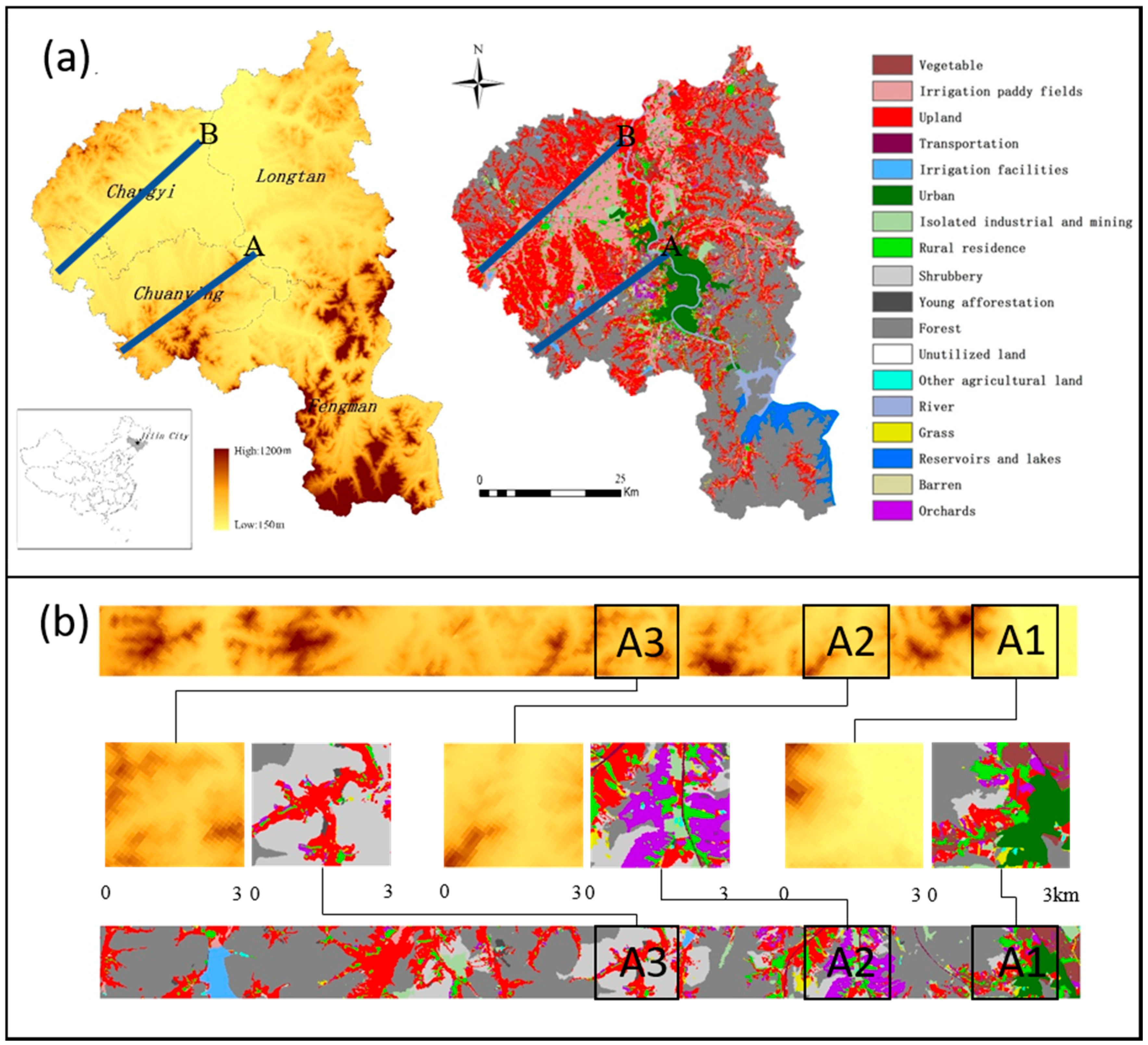
2.1. Data

The study area was located at 42°31′N–44°40′N, 125°40′E–127°56′E, Jilin Province, China. The Songhua River originating from the Changbai Mountains crosses the center of the metropolitan area before turning north into Russia. The land classification data were recorded from the land use survey of Jilin City, China in 2005 with the resolution 20 m and the terrain of Jilin slopes downward gradually from the southeast to the northwest (Figure 1). The topography factors used in this paper were elevation, slope, and aspect from the SRTM data with the resolution 90 m. The aspect was divided into five grades based on the azimuth: 0–22.5° and 337.5–360°, 22.5–67.5° and 292.5–337.5°, 67.5–112.5° and 247.5–292.5°, 112.5–157.5° and 202.5–247.5°, 157.5–202.5° (assigning the value as 1, 2, 3, 4 and 5, respectively).

According to the variation in terrain undulation and land use, A and B profiles (30 and 35 km in length, respectively) in the peri-urban area were selected; this covered nearly all of the land-use types in Jilin City (Figure 1). Profile A was located west of the downtown area and displayed a rather complex terrain, and the number of land use types gradually declined with distance from the urban region. Profile B was located in the Changyi District and had a relatively flat terrain and less varied land use.

Considering the effectivity of landscape metrics quantifying land use change and analyzing the correlation between landscape pattern and topography, the following landscape metrics were selected (

Table 1. Algorithm of some landscape metrics [28].

Landscape Metrics	Metrics Calculation Formula	Instructions
ED	$ED=\frac{E}{A}{10}^4$	E is the total length of patch edges in landscape. A is the total landscape area.
SHDI	$SHDI=-{\displaystyle \sum _{k=1}^n}{P}_k\ln \left(P_k\right)$	Pk equals the plane area of class k, divided by the landscape area.
PAFRAC	$PAFRAC=\frac{2\ast \left[\left(N{\sum }_{i=1}^m{\sum }_{j=1}^{n}ln{p}_{ij}^2\right)-{\left({\sum }_{i=1}^m{\sum }_{j=1}^{n}ln{p}_{ij}\right)}^2\right]}{\left[N{\sum }_{i=1}^m{\sum }_{j=1}^n\left(ln{a}_{ij}\ast ln{p}_{ij}\right)\right]-\left[\left({\sum }_{i=1}^m{\sum }_{j=1}^{n}ln{p}_{ij}\right)\left({\sum }_{i=1}^m{\sum }_{j=1}^{n}ln{a}_{ij}\right)\right]}$	$p_{ij}$ is the perimeter of patch ij, and $a_{ij}$ is the area of patch ij. m is the number of class i and n is the number of patches belong to the class i. N is the total number of patches in landscape.
Cohesion index	$Cohesion=\left[1-\frac{{\sum }_{j=1}^n{p}_{ij}}{{\sum }_{j=1}^n{p}_{ij}\sqrt{a_{ij}}}\right]{[1-\frac{1}{\sqrt{A}}]}^{-1}\ast 100$	$p_{ij}$ is the perimeter of patch ij, and $a_{ij}$ is the area of patch ij.
Proximity index	$Proximity={\sum }_{k=1}^n\frac{A_{ijk}}{D_{ijk}{}^2}$	$A_{ijk}$ is the area of patch ijk within a specified neighborhood. $D_{ijk}$ is the closest distance between patch ijk and patch ijk based on edge-to-edge distance, and k is the number of patches.

): The proximity and cohesion index were selected to describe the aggregation degree; the perimeter-area fractal dimension (PAFRAC) was selected to describe the shape complexity of the landscape; the edge density index (ED) was selected to describe the area-perimeter information; and Shannon’s diversity index (SHDI) was selected to describe the diversity of the landscape [2,12,28]. These landscape metrics, along with the urban-rural profiles, were calculated at the landscape level using a 1 km window size with the FRAGSTATS software [28], and the results were shown in Figure 2.

2.2. Pearson Correlation Coefficient

The Pearson correlation coefficient was calculated to evaluate the overall linear relationship [14]. Let X represent the landscape metric data and Y represent the topographical factor. The correlation r can be calculated as:

$$r=\frac{N\sum x_i{y}_i-\sum x_i\sum y_i}{\sqrt{N\sum x_i{}^2-{\left(\sum x_i\right)}^2}\sqrt{N\sum y_i{}^2-{\left(\sum y_i\right)}^2}}$$

(1)

A higher value of r indicates a greater correlation. A value of $r=1$ would indicate perfect similarity between landscape and topography data.

2.3. Continuous Wavelet Transform

Similar to the Fourier transform, the wavelet transform extends the time series from the spatial domain to the frequency domain [29]. By stretching the mother wavelet (e.g., the Haar, Mexican Hat, and Meyer and Morlet wavelets), the wavelet transform can obtain multi-scale characteristics of the signal [19]. The selection of wavelet function needs to follow the principles of zero-mean and convergence in both the spatial domain and the frequency domain [17].

As a complex symmetric function, Morlet wavelets can extract phase and amplitude information from the data [18,27]. In the spatial domain, the Morlet wavelet is defined as:

$$\psi \left(\eta \right)={\pi }^{-1/4}{e}^{i{\omega }_0\eta -0.5{\eta }^2}$$

(2)

where $\eta$ and ${\omega }_0$ denote the non-dimensional spatial parameter and non-dimensional frequency, respectively. When ${\omega }_0=6$, the Fourier period and scale are nearly equal ($\lambda =\frac{4\pi }{{\omega }_0+\sqrt{2+{\omega }_0^2}}s\approx 1.03s$), and this is advantageous for illustrating periodicity in the data [23].

By assuming a set of discrete sequences $X_n$ with same spatial sampling interval ${\delta }_t$, the CWT can be defined as the convolution of a discrete sequence and Morlet wavelets:

$$W_n^X\left(s\right)={\displaystyle \sum }_{n\prime =0}^{N-1}{X}_{n\prime }\psi \ast \left[\left(n\prime -n\right){\delta }_t/s\right], n=0\dots N-1$$

(3)

where $\ast$ indicates the complex conjugate. By changing the values of scale parameter $s$ and the translation parameter $n$, the variation characteristics of sequence $x_n$ along with scale and location can be obtained. In order to improve computational speed, the CWT is generally performed in the Fourier frequency domain [18]. The Fourier transform of discrete sequence $X_n$ is given by the following equation:

$${\widehat{x}}_k=\frac{1}{N}{\sum }_{n=0}^{N-1}{X}_n{e}^{-2\pi ikn/N}, k=0\dots N-1$$

(4)

According to the convolution theorem, the wavelet transform is inverse Fourier transform represented as [23]

$$W_n^X\left(s\right)={\displaystyle \sum }_{k=0}^{N-1}{\widehat{x}}_k\widehat{\psi }\ast (s{\omega }_k)e^{i{\omega }_{k}n\delta t}$$

(5)

where $\widehat{\psi }$ and ${\omega }_k$ represent the Fourier transform of Morlet basis and frequency, respectively. The wavelet transform of the discrete sequence can be calculated by Equation (5). As s increases, the spatial resolution is reduced and the frequency resolution rises, corresponding to low-frequency data. Since the Morlet wavelet is a complex function, the calculated value of the CWT is also complex. The result can be expressed as $a+ib$, where $a$ and $b$ represent the real part and imaginary part of the wavelet transform $W_n^X\left(s\right)$, respectively. The formula for wavelet transform phase is $\theta ={\mathit{tan}}^{-1}\frac{b}{a}$ with the range $\left[-\pi ,\pi \right]$, while the wavelet power spectrum is ${\left|W_n^x\right|}^2$ [10].

Given that the length of an urban-rural profile is finite, the errors existing at the beginning and end of the wavelet power spectrum need to be considered. The influence of the cone (COI) is caused by the discontinuity of discrete data at the boundary. This can be solved by the method of padding the end of spatial series with zeroes before the wavelet transform and then eliminating the added zeroes afterwards [18]. This phenomenon occurs in non-stationary data but not in a periodic sequence [10].

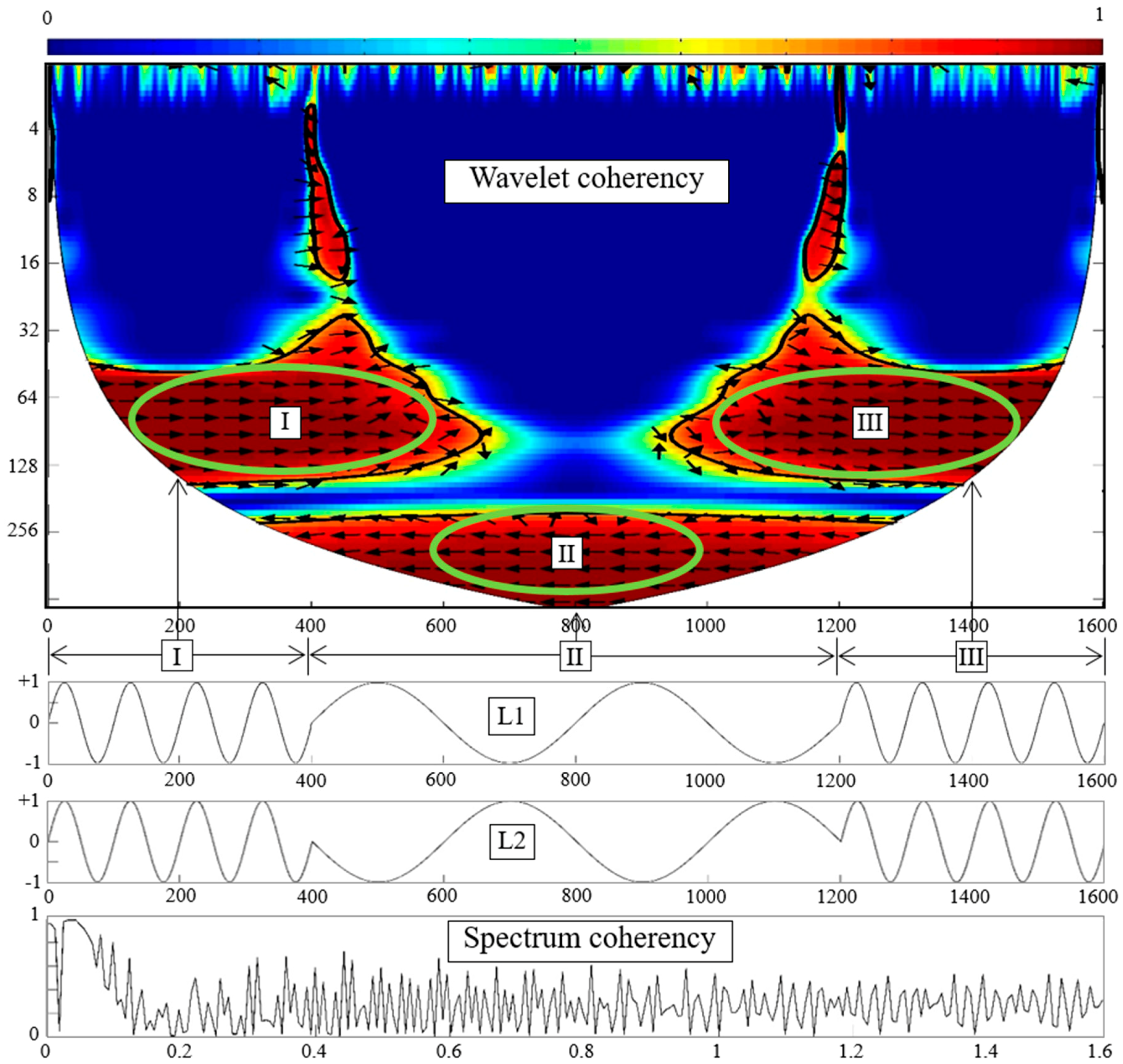
2.4. Wavelet Coherency Analysis

For two spatial series, the wavelet coherency method is quite useful for analyzing local linear correlation at a given location and spatial scale and for determining whether the occurrence of a frequency in sequence X is related to sequence Y at the same position (Figure 3). This analysis is similar to the traditional correlation coefficient method, while the wavelet coherency at multiple scales is more reliable compared with the single value obtained under the sampling scale [23]. A detailed definition of the wavelet coherency method is given in [27].

$$R_n^2=\frac{{\left|S\left(s^{-1}{W}_n^{XY}\right)\right|}^2}{S(s^{-1}{\left|W_n^X\right|}^2).S(s^{-1}{\left|W_n^Y\right|}^2)}$$

(6)

$W_n^{XY}$ is defined as $W^{XY}=W^X{W}^{Y\ast }$ to represent the cross-wavelet transform. The function $S$ is an operator smoothing the wavelet power spectrum in order to increase the degrees of freedom and enhance the confidence level of significant power regions [19]. For the Morlet wavelet, $S$ can be defined as [10]:

$$S\left(W\right)=S_{scale}\left(S_{space}\left(W\left(s,\tau \right)\right)\right)$$

(7)

where $S_{space}$ indicates smoothing along the spatial location and $S_{scale}$ indicates smoothing along the scale. The former is represented as [30]

$$S_{space}\left(W\left(s,\tau \right)\right)={\displaystyle \sum }_{k=0}^{N-1}{\left(W(s,\tau )\frac{1}{s\sqrt{2\pi }}\mathit{exp}\left(-\frac{{\left(\tau -x_k\right)}^2}{2s^2}\right)\right)|}_s$$

(8)

where the Fourier transform of the smoothing function $\frac{1}{s\sqrt{2\pi }}\mathit{exp}\left(-\frac{{\left(\tau -x_k\right)}^2}{2s^2}\right)$ is expressed as $\mathit{exp}\left(-2s^2{\omega }^2\right)$. According to the convolution theorem, Equation (8) can be written based on the fast Fourier transform and inverse Fourier transform as [14]:

$$S_{space}\left(W\left(s,\chi \right)\right)=IFFT\left(FFT\left(W\left(s,\tau \right)\right)\right(\mathit{exp}\left(-2s^2{\omega }^2\right))$$

(9)

$S_{scale}$ can be defined as

$$S_{scale}W(s_k,\chi )=\frac{1}{2m+1}{\displaystyle \sum }_{j=k-m}^{k+m}{(S_{space}\left(W\left(s_j,\chi \right)\right).\Pi \left(0.6s_j\right))|}_{\chi }$$

(10)

where $\Pi$ represents rectangle function and parameter 0.6 is the empirical value of de-correlation length based on Morlet wavelet [10,18].

According to the trend of standard deviations of calculated wavelet coherency, three main scale intervals (small, medium, and large scales) and the relative average correlation-location curves of the variables could be defined to study the correlation characteristics between topography and land use data at different locations. At small scales, the standard deviations changed slightly, and the correlation features were weak and scattered because landscape patches were more affected by some small topographical features, like valleys and hillsides. At medium scales, the standard deviations show larger fluctuation, and the changes in land use were related to the topography at a specific location, such as A2 and A3 regions in profile A (Figure 1). At large scales, if the study area was wide enough without the effect of COI, the standard deviations remained nearly unchanged and close to zero. Strong positive correlations were very apparent throughout the study area; this was influenced by the alternate mountains and plains rather than the topographic features at small or medium scales.

2.5. Test of Significance

Traditional significance tests of hypotheses are not suitable for the coherence analysis due to the redundancy caused by a non-orthogonal wavelet function in the CWT [27]. This study applied the Monte Carlo method to test the significance of the coherencies. The first-order autocorrelation coefficients for paired samples (topography factor and landscape metric) were calculated to generate a new red noise spectrum replacing the original data [31]. Then, 1000 realizations of the spatial series were generated, and the wavelet coherency of each realization at each scale and location was calculated. After that, the calculated 1000 wavelet coherencies at each scale were arranged in increasing order. Based on the order results, 95% of the calculated values were below the 950th wavelet coherency value; this then defined the 95% confidence interval at relevant scale and location [10,14]. If the statistical result falls into the 95% confidence interval, then it is possible for the landscape metric and topography factor to be perfectly correlated at that scale. If the statistical result does not lie within the confidence interval, the correlation between variables can be an unreliable indicator of causality [27]. The correlations shown in the wavelet coherency diagram indicate whether and how strong the landscape metrics are related to the topography factor. The continuous wavelet transform, coherency analysis and Monte Carlo significance test were completed using the MATLAB codes written by Grinsted et al. [27].

3. Results

3.1. Overall Pearson Correlation

Table 2. The correlation coefficients between landscape metrics and topography factors (* p < 0.01, ** p < 0.05).

Landscape Metric	DEM	Slope	Aspect
Proximity_A	−0.161 *	−0.204 *	0.008
PAFRAC_A	−0.612 *	−0.416 *	−0.172 *
Cohesion_A	0.661 *	0.427 *	0.193 *
ED_A	−0.672 *	−0.495 *	−0.166 *
SHDI_A	−0.753 *	−0.462 *	−0.195 *
Proximity_B	−0.103 **	−0.030	−0.002
PAFRAC_B	0.230 *	−0.022	0.015
Cohesion_B	−0.249 *	0.001	0.001
ED_B	0.273 *	−0.021	0.020
SHDI_B	0.234 *	0.113 **	−0.069

lists the overall Pearson correlation coefficients between landscape metrics and topography factors. For profile A, none of the employed metrics were linearly dependent on the aspect, and the linear correlation between the metrics and DEM was stronger than that for slope, with ranges of 0.612 to 0.753 and 0.416 to 0.495, respectively. In contrast to other metrics, the cohesion index had a positive linear correlation with both DEM and slope. There was no significant linear correlation between proximity index and topography factors, while the SHDI was the most sensitive index for describing the influence of elevation and slope on the landscape heterogeneity, with coefficients of −0.753 and −0.462, respectively. As for profile B, each coefficient was below 0.3, indicating that there was no significant linear correlation between the variables. Even when the correlation coefficient was effective in evaluating the overall linear correlation, the scales and locations of the correlations along the profiles could not be identified.

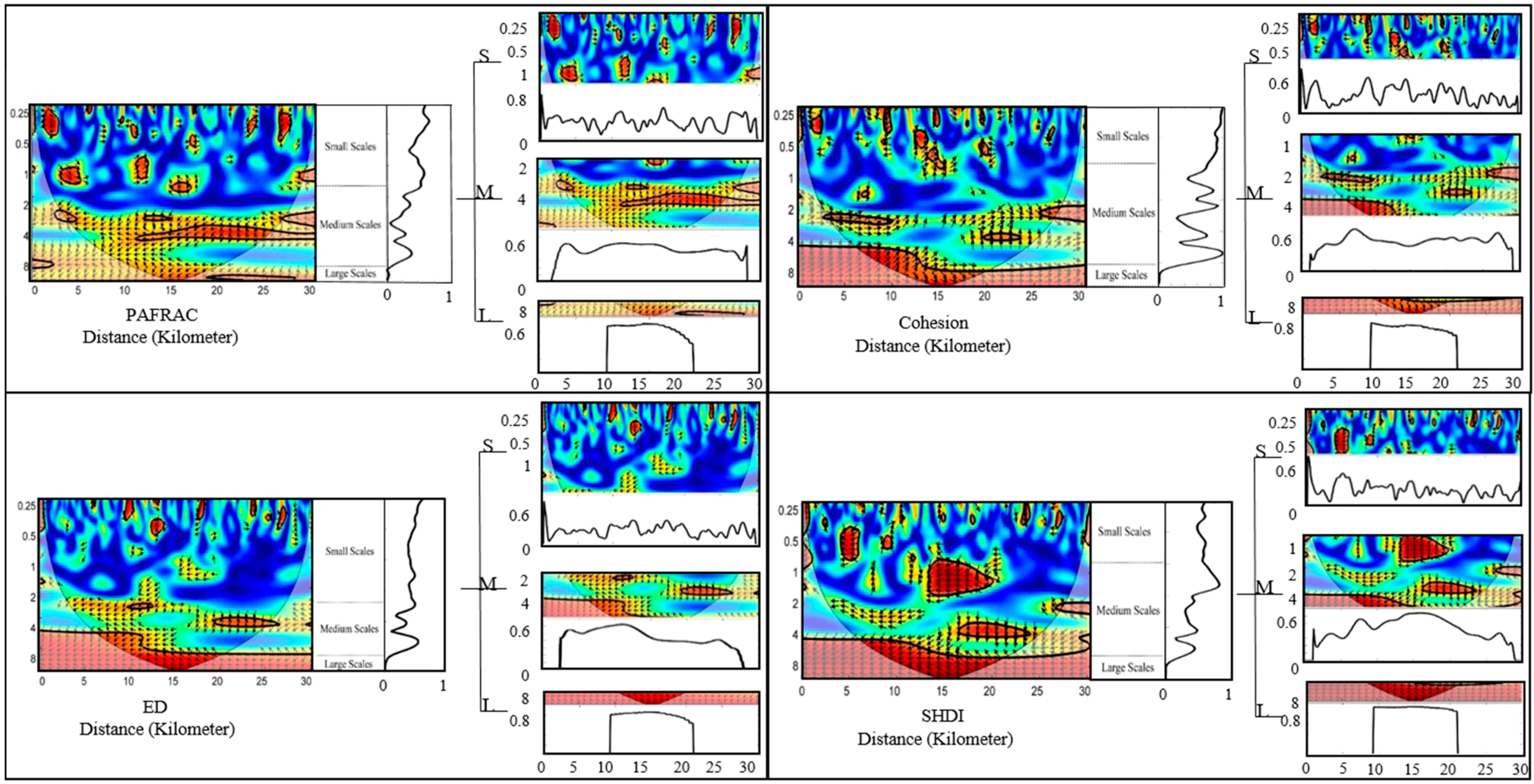
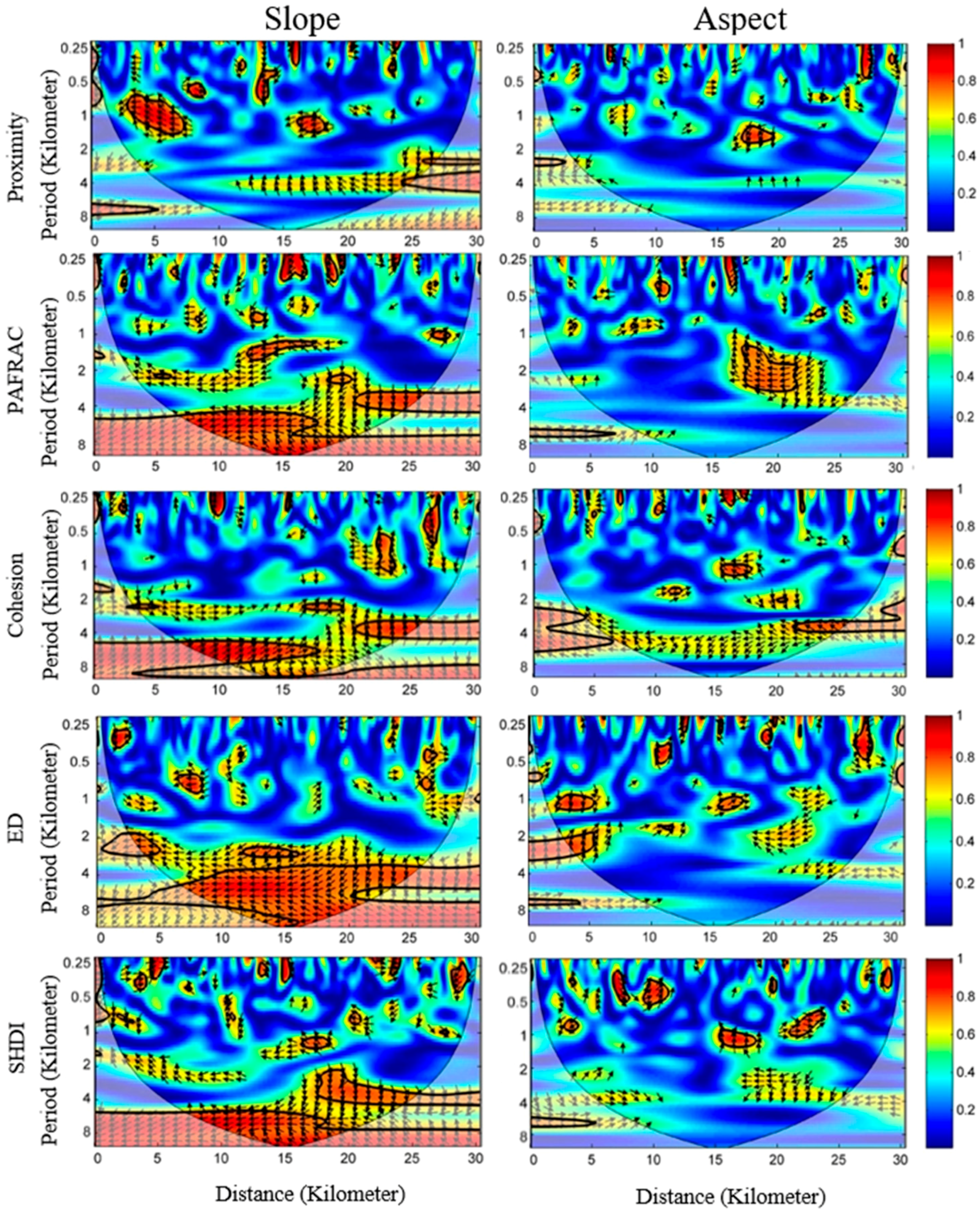
3.2. The Wavelet Coherencies between Topography Factors and Landscape Indices

Along profile A, 303 sampling points with the same interval were selected, and the local coherencies between landscape metrics and elevation were calculated at 69 scales (Figure 4). According to the wavelet coherencies and variation in standard deviation of the calculated values at each scale, three main scale intervals for each landscape metric (except proximity index) were defined (

Table 3. The main scale intervals of selected landscape metrics in profile A.

Scale Division	PAFRAC (km)	Cohesion (km)	ED (km)	SHDI (km)
Small Scales	0.25–1.5	0.25–1	0.25–2	0.25–1
Medium Scales	1.5–8	1–8	2–8	1–8
Large Scales	>8	>8	>8	>8

), and relative average correlation-location curves at different scale intervals were obtained (Figure 4).

The correlations between the PAFRAC index and elevation exhibited obvious multi-scale characteristics. As shown in Figure 4, there were no significant coherencies at small scales. At medium scales, the related features changed with location, with the average values of the correlation-location curve from A2 and A3 regions all over 0.5. The strong correlation in the A2 region resulted from the major road crossing the valley; this feature strongly affected the land use pattern in this area. In the A3 region, the intense terrain undulation may have led to a low complexity value of the landscape by influencing the patch length and number, and especially the occurrence of large patches. As scale increased, the calculated pixels at small or medium scales combined to form a new cell with a larger size, meaning that the micro-topography elements were replaced by larger fluctuations. This change of scale would enhance the correlation between landscape pattern and elevation. At large scales, the index was negatively linked to elevation, with the average correlation values above 0.6 throughout the study area. This indicated that the PAFRAC index was sensitive enough to describe the influence of elevation on landscape at this scale.

The strength of correlation between the cohesion index and elevation overtook the PAFRAC index in total. At small scales, the correlation between variables lacked regularity. At medium scales, the correlation was controlled by the topography of local positions, for example, in the A2 region where correlation-location curve peaked with the average value over 0.5. The correlation period in the A3 region indicated a gradual upward trend from 4 to 7 km, which may have been caused by the distance from the downtown area. At a certain distance from the center of the downtown area, human behavior dominates the landscape pattern. This results from, for example, the exploitation of constructive and non-constructive land, leading to many small patches, and the landscape can be more fragmented. As sampling points became farther away from urban area, the influence of topography strengthened along with the weakening influence of human activities. A more varied topography may lead to a simpler landscape pattern because human activities are impeded in these areas. At larger scales, the average values in the location curve exceeded 0.7. This significant correlation indicated that the cohesion index could be applied to describe the influence of topography on landscape aggregation degree. As the scale increased, some large fluctuations of metric and elevation appeared, while small fluctuations in the terrain observed at small and medium scales became weakened or disappeared. A similar phenomenon also occurs in the correlation relationship between the ED index and elevation.

The correlation between the SHDI index and elevation exceeded the other three metrics. At medium scales, the SHDI index was negatively related to the elevation in the A3 region. Compared with the other metrics, a larger significant area in the A3 region indicated a stronger sensitivity to describing the terrain variation affecting the landscape pattern in this scale-location range. As for the cohesion index, the related period between SHDI index and elevation showed a gradually increasing trend. At large scales, the SHDI index was negatively related to elevation in the total study area. As the topography became more complex, the numbers of patches and patch types both showed a descending trend, leading to the increasing area of the dominant type. In addition to elevation, the wavelet coherencies between landscape metrics and other topography factors (slope and aspect) along Profile A were calculated (Figure 5). On the whole, the responses of landscape metrics to different topographic factors differed. In comparison to the random and scattered correlation features with aspect, the landscape metrics were significantly related to elevation and slope, indicating that the landscape was more likely to be dominated by elevation and slope rather than aspect within a certain range. This phenomenon might result from the terrain variation within the total study area. Even though the terrain of profile A was more varied compared with that of profile B, the degree of terrain variation was still limited in that the sunlight intensity could not generate a large influence on the variation of land use patterns at different locations within the region.

Along profile B, 349 sampling points were selected with an interval of 100 m. The results are shown in Figure 6. The wavelet coherencies between topographical factors and landscape indices lacked regularity at each scale, and the weakly related characteristics were more influenced by human activity, e.g., traffic and human habitation.

4. Discussion

As a multidimensional variable, topography affects the landscape pattern over a wide range of scales and locations [14,32,33]. Significant correlations within regions and scales change according to the research object and the range of the study area [8]. To some microorganisms or reptiles, the correlations at small scales can be more significant than those at larger scales, and the significant regions at different scales can be displayed in smaller units, such as meters or centimeters [8]. Given that the calculated correlation features were only identified in our study area, more research is needed to judge whether the results would be effective in other regions.

Massive amounts of empirical research have demonstrated the existence of spatial correlation and its scale dependency in landscape patterns and ecological processes [2,7,34]. Although some previous studies have analyzed the relationship between landscape pattern and topography or other influencing factors [5,35,36], our study has focused more attention on the identification of scales and location using wavelet analysis; the results have essential implications for a detailed understanding of the relationship between landscape patterns and ecological processes. The information obtained from a single spatial scale is limited, and the features of correlation may vary with the location at different scales [13,24]. The wavelet method is very effective in processing complex land use data and relating the landscape pattern with scale at a local position; this is useful for detecting the hierarchy, aggregation, and other important landscape features over a wide range of scales and locations [14,19]. Considering the multi-scale property, the application field of wavelet analysis could be further expanded. For example, a current topic of interest in the study of urban heat islands (UHI) is the influence of factors, such as the vegetation and water on the strength of UHI. The wavelet method can analyze periodic and correlated features with factors at different scales and locations, avoiding the limitation of a single scale and a single area [13].

Even using wavelets, there are still some deficiencies. The selected landscape metrics may show correlations mainly caused by similarities in mathematical formulas, although the metrics may have different ecological meanings in describing the landscape pattern. The selected size of the moving window used in calculating the landscape metrics also influences the results. The resolution of DEM and other related topography data are equal to 90 m, lower than the land classification data measured using GPS. In fact, higher resolution concerning land use and topography will yield more detailed information, such as the degree of terrain undulation, which may lead to wider options of the chosen spatial scales and more credibly correlated characteristics. Both of the above deficiencies, regardless of size selection and resolution, refer to the scale issue and would benefit from further study. The results presented herein suggest that multi-scale and multi-location landscape features can be identified using the wavelet method.

5. Conclusions

This study analyzed the similarities between topographical factors and landscape metrics using the Pearson correlation coefficient, identified the scales and locations of the correlations between variables using the wavelet coherency method in urban-rural profiles, and obtained average correlation-location curves under different scale intervals. According to the experimental results, we may draw the conclusions that follow.

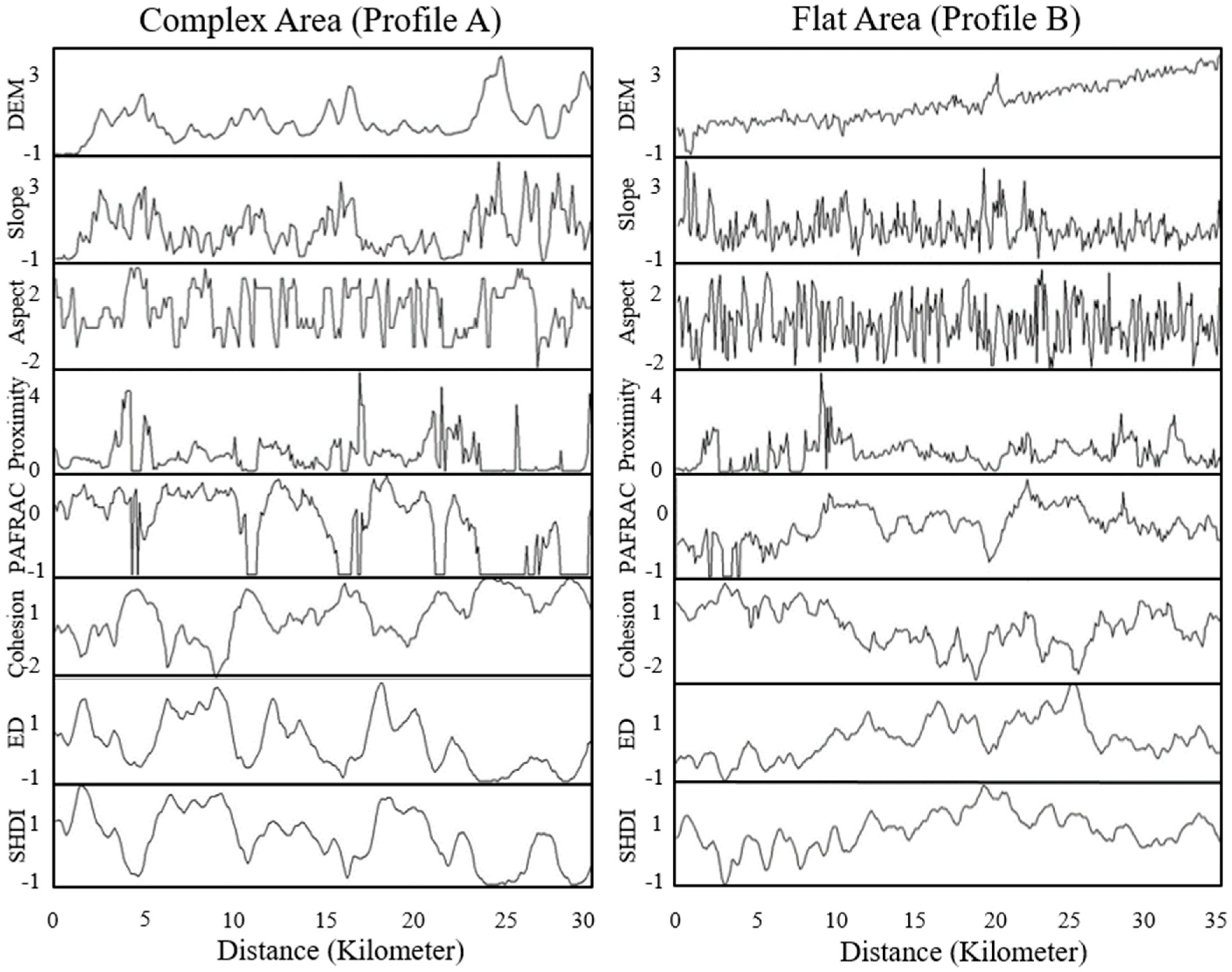
• The wavelet analysis was more sensitive than the Pearson correlation coefficient for describing the correlations between landscape patterns and topography at different scales, and the topography was much more related to land use pattern in the complex area than that in the flat area.
• Landscape metrics should not be chosen randomly to study ecological phenomena. This is because some landscape metrics were not sensitive to the terrain variation (e.g., the proximity index), while other selected metrics displayed obvious multi-scale features in describing the influence of the 3D terrain (mainly the elevation and slope) on the landscape pattern.
• The multi-location correlation characteristics at different scales were measured along urban-rural profiles. For example, the influence of traffic lines on the land use distribution within a neighborhood space was indicated only at medium scales in the A2 region, while the correlation was extremely weak at smaller scales and extremely strong at larger scales for the total study area.
• The variation of the correlation period between topography and landscape metrics, especially the decrease shown in the A3 region, can be seen as important evidence that the main influencing factors of landscape pattern gradually changed from human influences to topography.
• The identification of multiple scales and locations using the wavelet method supplies us with new insights into the relationship between landscape heterogeneity and topography. However, this kind of method is still too complex, and the ecological interpretation of wavelet coherencies needs to be supplemented as well as have a more accurate division strategy of scale.

References

1. Goodchild, M.F. Spatial Autocorrelation; Geo Books: Norwich, UK, 1986; Volume 47. [Google Scholar]
2. Wu, J. Effects of changing scale on landscape pattern analysis: Scaling relations. Landsc. Ecol. 2004, 19, 125–138. [Google Scholar] [CrossRef]
3. Fissore, C.; Dalzell, B.J.; Berhe, A.A.; Voegtle, M.; Evans, M.; Wu, A. Influence of topography on soil organic carbon dynamics in a Southern California grassland. Catena 2017, 149, 140–149. [Google Scholar] [CrossRef]
4. Hais, M.; Chytrý, M.; Horsák, M. Exposure-related forest-steppe: A diverse landscape type determined by topography and climate. J. Arid Environ. 2016, 135, 75–84. [Google Scholar] [CrossRef]
5. Ivanov, V.Y.; Bras, R.L.; Vivoni, E.R. Vegetation-hydrology dynamics in complex terrain of semiarid areas: 2. Energy-water controls of vegetation spatiotemporal dynamics and topographic niches of favorability. Water Resour. Res. 2008, 44, 380–384. [Google Scholar] [CrossRef]
6. Fernandes, M.R.; Aguiar, F.C.; Ferreira, M.T. Assessing riparian vegetation structure and the influence of land use using landscape metrics and geostatistical tools. Landsc. Urban Plan. 2011, 99, 166–177. [Google Scholar] [CrossRef]
7. Pautasso, M. Scale dependence of the correlation between human population presence and vertebrate and plant species richness. Ecol. Lett. 2007, 10, 16–24. [Google Scholar] [CrossRef] [PubMed]
8. Ekroos, J.; Ödman, A.M.; Andersson, G.K.; Birkhofer, K.; Herbertsson, L.; Klatt, B.K.; Rundlöf, M. Sparing land for biodiversity at multiple spatial scales. Front. Ecol. Evol. 2016, 3, 145. [Google Scholar] [CrossRef]
9. Mairota, P.; Cafarelli, B.; Labadessa, R.; Lovergine, F.; Tarantino, C.; Lucas, R.M.; Didham, R.K. Very high resolution Earth observation features for monitoring plant and animal community structure across multiple spatial scales in protected areas. Int. J. Appl. Earth Observ. Geoinform. 2015, 37, 100–105. [Google Scholar] [CrossRef]
10. Si, B.C.; Zeleke, T.B. Wavelet coherency analysis to relate saturated hydraulic properties to soil physical properties. Water Resour. Res. 2005, 41, 303–306. [Google Scholar] [CrossRef]
11. Grimm, N.B.; Pickett, S.T.; Hale, R.L.; Cadenasso, M.L. Does the ecological concept of disturbance have utility in urban social–ecological–technological systems? Ecosyst. Health Sustain. 2017. [Google Scholar] [CrossRef]
12. Wu, J. Landscape Ecology: Pattern, Process, Scale and Hierarchy; Higher Education Press: Beijing, China, 2000. [Google Scholar]
13. Ma, Q.; Wu, J.; He, C. A hierarchical analysis of the relationship between urban impervious surfaces and land surface temperatures: Spatial scale dependence, temporal variations, and bioclimatic modulation. Landsc. Ecol. 2016, 31, 1139–1153. [Google Scholar] [CrossRef]
14. Biswas, A.; Si, B.C. Scales and locations of time stability of soil water storage in a hummocky landscape. J. Hydrol. 2011, 408, 100–112. [Google Scholar] [CrossRef]
15. Hiebeler, D.E.; Houle, J.; Drummond, F.; Bilodeau, P.; Merckens, J. Locally dispersing populations in heterogeneous dynamic landscapes with spatiotemporal correlations. I. block disturbance. J. Theor. Biol. 2016, 407, 212–224. [Google Scholar] [CrossRef] [PubMed]
16. Zhou, T.; Wu, J.; Peng, S. Assessing the effects of landscape pattern on river water quality at multiple scales: A case study of the Dongjiang River watershed, China. Ecol. Indic. 2012, 23, 166–175. [Google Scholar] [CrossRef]
17. Farge, M. Wavelet transforms and their applications to turbulence. Annu. Rev. Fluid Mech. 1992, 24, 395–458. [Google Scholar] [CrossRef]
18. Torrence, C.; Compo, G.P. A practical guide to wavelet analysis. Bull. Am. Meteorol. Soc. 1998, 79, 61–78. [Google Scholar] [CrossRef]
19. Saunders, S.C.; Chen, J.; Drummer, T.D.; Gustafson, E.J.; Brosofske, K.D. Identifying scales of pattern in ecological data: A comparison of lacunarity, spectral and wavelet analyses. Ecol. Complex. 2005, 2, 87–105. [Google Scholar] [CrossRef]
20. Yang, Y.; Zhou, Q.; Gong, J.; Wang, Y. Gradient analysis of landscape spatial and temporal pattern changes in Beijing metropolitan area. Sci. China Technol. Sci. 2010, 53, 91–98. [Google Scholar] [CrossRef]
21. Modica, G.; Vizzari, M.; Pollino, M.; Fichera, C.R.; Zoccali, P.; Di Fazio, S. Spatio-temporal analysis of the urban–rural gradient structure: An application in a Mediterranean mountainous landscape (Serra San Bruno, Italy). Earth Syst. Dyn. 2012, 3, 263–279. [Google Scholar] [CrossRef]
22. Fichera, C.R.; Modica, G.; Pollino, M. GIS and remote sensing to study urban-rural transformation during a fifty-year period. In International Conference on Computational Science and Its Applications; Springer: Berlin/Heidelberg, Germany, 2011; pp. 237–252. [Google Scholar]
23. Vadrevu, K.P.; Choi, Y. Wavelet analysis of airborne CO2 measurements and related meteorological parameters over heterogeneous landscapes. Atmos. Res. 2011, 102, 77–90. [Google Scholar] [CrossRef]
24. Chave, J. The problem of pattern and scale in ecology: What have we learned in 20 years? Ecol. Lett. 2013, 16, 4–16. [Google Scholar] [CrossRef] [PubMed]
25. Saunders, S.C.; Chen, J.; Crow, T.R.; Brosofske, K.D. Hierarchical relationships between landscape structure and temperature in a managed forest landscape. Landsc. Ecol. 1998, 13, 381–395. [Google Scholar] [CrossRef]
26. Biswas, A. Landscape characteristics influence the spatial pattern of soil water storage: Similarity over times and at depths. Catena 2014, 116, 68–77. [Google Scholar] [CrossRef]
27. Grinsted, A.; Moore, J.C.; Jevrejeva, S. Application of the cross wavelet transform and wavelet coherence to geophysical time series. Nonlinear Processes Geophys. 2004, 11, 561–566. [Google Scholar] [CrossRef] [Green Version]
28. McGarigal, K.; Cushman, S.A.; Neel, M.C.; Ene, R. FRAGSTATS: Spatial Pattern Analysis Program for Categorical Maps. Computer Software Program Produced by the Authors at the University of Massachusetts, Amherst (2002). Available online: http://www.umass.edu/landeco/research/fragstats/fragstats.html (accessed on 1 April 2018).
29. Kumar, P.; Foufoula-Georgiou, E. Wavelet analysis for geophysical applications. Rev. Geophys. 1997, 35, 385–412. [Google Scholar] [CrossRef] [Green Version]
30. Torrence, C.; Webster, P.J. The annual cycle of persistence in the El Nño/Southern Oscillation. Q. J. R. Meteorol. Soc. 1998, 124, 1985–2004. [Google Scholar] [CrossRef]
31. Pardo-Igúzquiza, E.; Rodríguez-Tovar, F.J. The permutation test as a non-parametric method for testing the statistical significance of power spectrum estimation in cyclostratigraphic research. Earth Planet. Sci. Lett. 2000, 181, 175–189. [Google Scholar] [CrossRef]
32. Dietrich, W.E.; Wilson, C.J.; Montgomery, D.R.; McKean, J. Analysis of erosion thresholds, channel networks, and landscape morphology using a digital terrain model. J. Geol. 1993, 101, 259–278. [Google Scholar] [CrossRef]
33. Thompson, J.A.; Bell, J.C.; Butler, C.A. Digital elevation model resolution: Effects on terrain attribute calculation and quantitative soil-landscape modeling. Geoderma 2001, 100, 67–89. [Google Scholar] [CrossRef]
34. Campagnaro, T.; Frate, L.; Carranza, M.L.; Sitzia, T. Multi-scale analysis of alpine landscapes with different intensities of abandonment reveals similar spatial pattern changes: Implications for habitat conservation. Ecol. Indic. 2017, 74, 147–159. [Google Scholar] [CrossRef]
35. Lundholm, J.T. Plant species diversity and environmental heterogeneity: Spatial scale and competing hypotheses. J. Veg. Sci. 2009, 20, 377–391. [Google Scholar] [CrossRef]
36. Djebou, D.C.S.; Singh, V.P.; Frauenfeld, O.W. Analysis of watershed topography effects on summer precipitation variability in the southwestern united states. J. Hydrol. 2014, 511, 838–849. [Google Scholar] [CrossRef]
Figure 1. The digital elevation model (DEM) and landscape of Jilin City and the locations of landscape profiles A and B (a). The correlations between landscape and topography at specific locations A1, A2, and A3 within profile A are shown in (b). A1 is located in the north of the downtown area and includes more diverse land use types in its northern part. A2 has two major roads across the valley, and the land use types are distributed symmetrically along the traffic lines. A3 represents the mountain area, and the number of landscape patches is less than in the other samples. The area is located approximately 15 km from the downtown area.
Remotesensing 10 01653 g001
Figure 2. The variations of topographical factors and landscape indices after zero-mean normalization in profiles (A) complex area and (B) flat area.
Remotesensing 10 01653 g002
Figure 3. A wavelet coherency and spectrum coherency diagram. The simulated data L1 and L2 have a perfect similarity between the locations [0, 400] and [1200, 1600] with the correlation coefficient 1, and a negative correlation between the locations [400, 1200] with the coefficient −1. The overall correlation coefficient is thus equal to zero with no apparent explanation. In the wavelet diagram, the X axis represents the location in the profile; the Y axis represents the correlation period; the thick black line represents the 95% confidence level; the solid black line represents the COI, and the direction of the arrow represents the type of correlation. The right-directed arrow indicates a positive correlation, while the left-directed arrow indicates a negative correlation. The Fourier period is approximately the same as the scale. It can be seen that there is a significant positive correlation within the range of scales [40, 128] in the areas I and III as well as a significant negative correlation in the area II when the scale exceeds 256. In the spectrum coherency diagram, the X and Y axes represent the normalized frequency and correlation coefficient, respectively, and the chart shows a clear scale relationship without location information.
Remotesensing 10 01653 g003
Figure 4. The wavelet coherencies between landscape indices and elevation in profile A. The capital letters S, M, and L represent small, medium, and large scales, respectively. The figures on their left represent the wavelet coherencies and standard deviation curves. The captions describe the relative scale intervals. The figures to the right of the letters represent the wavelet diagrams and average correlation-location curves corresponding to small scales, medium scales, and large scales from top to bottom.
Remotesensing 10 01653 g004
Figure 5. The wavelet coherencies between landscape metrics and other topographical factors (slope and aspect) in profile A.
Remotesensing 10 01653 g005
Figure 6. The wavelet coherencies between landscape metrics and topographical factors in profile B.
Remotesensing 10 01653 g006