1. Introduction
The Earth’s hydrological cycle is perhaps the most important physical process for sustaining life. However, capturing the quantitative details of it on a global scale is a challenge, mostly because of sparse measurements. Satellite observations, especially those from low-earth orbiting satellites that provide global coverage, have proven to be vital in contributing information on several key parameters unattainable from surface observations.
Passive microwave measurements have been available on satellites from the 1970s, on research satellites flown by the National Aeronautics and Space Administration (NASA). Early sensors included the Electrically Scanning Microwave Radiometer (ESMR) and Scanning Multichannel Microwave Radiometer (SMMR) instruments. Data from those instruments allowed construction of the first global climatologies of sea-ice, snow cover, water vapor, and rainfall [
1,
2]. Since then, several other sensors have been flown to retrieve hydrological products for both operational weather applications (e.g., the Special Sensor Microwave/Imager—SSM/I; the Advanced Microwave Sounding Unit—AMSU) and climate applications (e.g., the Advanced Microwave Scanning Radiometer—AMSR; the Tropical Rainfall Measurement Mission Microwave Imager—TMI; the Global Precipitation Mission Microwave Imager—GMI).
In this paper, the focus is on measurements from AMSU-A, AMSU-B, and the Microwave Humidity Sounder (MHS). These sensors have been in operation since 1998, with the launch of NOAA-15, and are also on NOAA-16, -17, -18, -19, and the MetOp-A and -B satellites. A data set called the “Hydrological Bundle” is a climate data record (CDR) that utilizes brightness temperatures from fundamental CDRs (FCDRs) to generate thematic CDRs (TCDRs) [
3,
4]. The TCDRs are generated using the Microwave Surface and Precipitation Products System (MSPPS) package, and produces a set of products including total precipitable water (TPW), cloud liquid water (CLW), sea-ice concentration (SIC), land surface temperature (LST), land surface emissivity (LSE) for 23, 31, 50 GHz, rain rate (RR), snow cover (SC), ice water path (IWP), and snow water equivalent (SWE) [
5]. More details, including the Climate Algorithm Theoretical Basis Document (C-ATBD), can be found in the documentation of the CDR at
https://www.ncdc.noaa.gov/cdr/atmospheric/hydrological-properties.
The purpose of this paper is to (1) provide a description of the hydrological bundle CDR (hereafter referred to as HBC); (2) provide an assessment of the HBC; and (3) provide a comparison of the HBC with certain companion data sets and CDRs. In order for end users of the data sets to understand the strengths and weaknesses of the HBC, comparisons are done to evaluate consistencies between the HBC and similar data sets. Consistencies suggest reliability, while inconsistent features indicate where more in-depth evaluation is needed to understand them.
This paper is organized as follows:
Section 2 gives the data set descriptions,
Section 3 provides some comparisons with comparable data sets, and
Section 4 offers conclusions and recommendations.
2. Data and Methods
2.1. Hydrological Bundle CDR (HBC)
The Advanced Microwave Sounding Unit-A and -B (AMSU-A/B) and Microwave Humidity Sounder (MHS) are cross-track scanning sensors designed to measure earth scene radiances; its primary design function is to provide temperature (AMSU-A) and water vapor (AMSU-B/MHS) profiling of the atmosphere. AMSU-A/B was first flown on the NOAA-15 satellite (beginning July 1998). The most complete references to the sensor can be found in [
6,
7].
Table 1 shows the instrument characteristics for AMSU-A/B MHS level 2 data.
The HBC data period of record begins in 2000, with monthly updates. Beginning with that year, there are multiple satellites with the advanced sensors that were first flown on NOAA-15. It contains a 48 km (AMSU-A) and 16 km (AMSU-B/MHS) nadir global resolution. The period of record for the hydrological bundle CDR is 2000–2016, and will be routinely expanded throughout the lifespan of the satellites.
Table 2 lists when data are most reliable, while
Table 3 provides attributes of the TCDRs. One caveat is that the FCDRs must be of sufficient quality, especially as sensors degrade over time and cannot be reliably adjusted, as is the case for earlier data periods. Data from degraded sensors must be excluded from the CDRs to maintain their quality and pass rigid quality control procedures. Due to radio frequency interference (RFI) issues with AMSUI-B on NOAA-15, data prior to 2000 is difficult to correct, and is presently excluded from the HBC. It is possible that, in a future version, the data can be extended back to 1998. NOAA-17 was impacted by a solar flare early in its operation, which impacted several channels on AMSU-A and AMSU-B. This is why the HBC has a short period of record, even though other instruments on the satellite operated for several more years.
As of 2016, TCDRs are only generated for NOAA-18, NOAA-19, and MetOp-A. It should be noted that CDRs are feasible for MetOp-B and MetOp-C (2018 launch), however, these two satellites are not part of the original hydrological bundle.
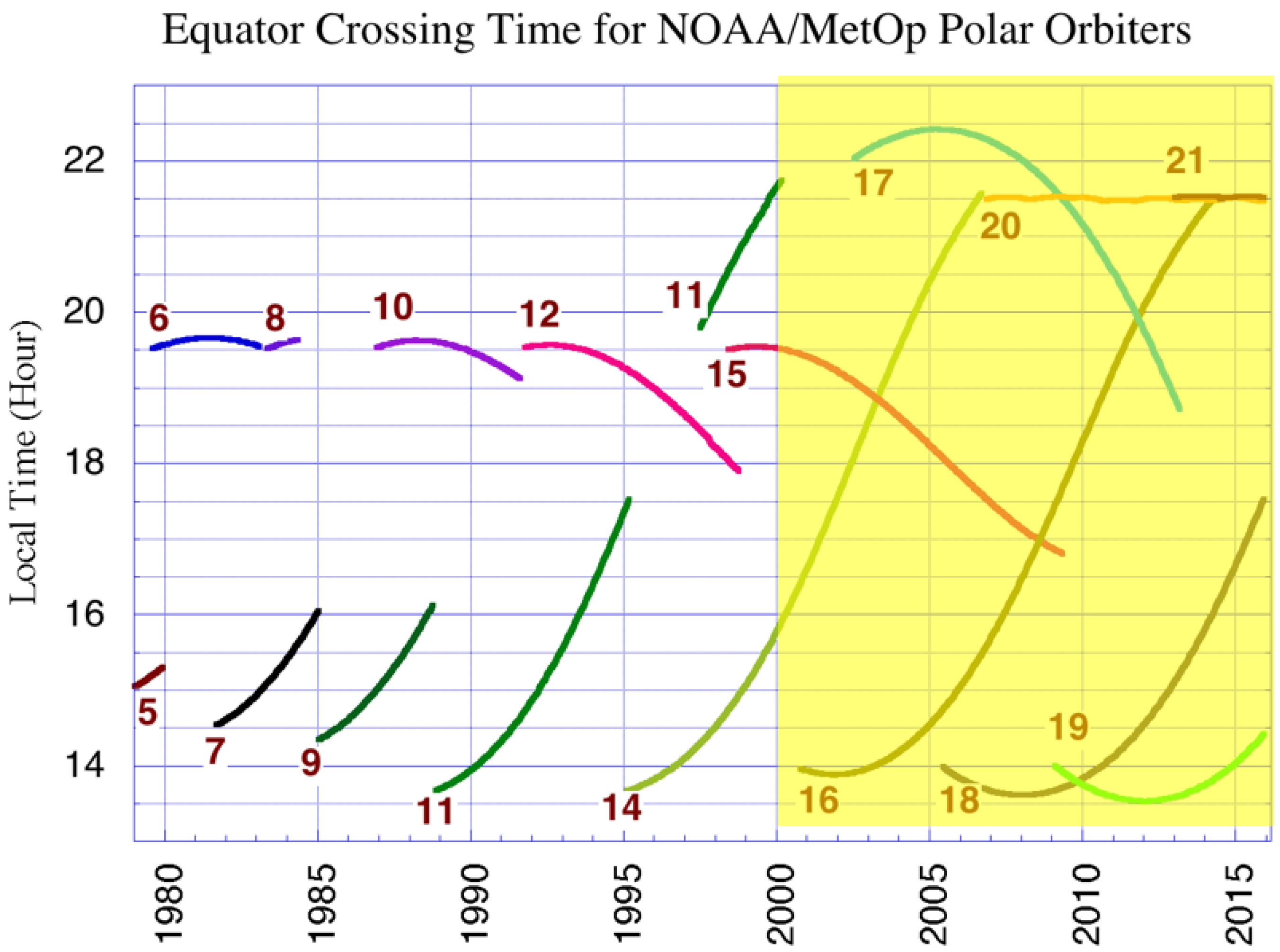
Figure 1 provides information on the equatorial crossing times of NOAA and MetOp satellites.
The AMSU sensor package was replaced with the Advanced Technology Microwave Sounder (ATMS), the first of which was flown on the S-NPP satellite (from 2012) and, most recently, NOAA-20 (from November 2017). Although beyond the scope of this project, the HBC could be expanded to include ATMS, which provides the CDR the opportunity to expand the period of record. In addition, these data provide an opportunity to develop CDRs that can contribute to other satellite time series with similar capabilities.
Finally, similar products have been produced from other passive microwave satellite series. In particular, the DMSP Special Sensor Microwave Imager (SSM/I), first placed into operation in 1987, has been used in numerous studies to generate CDR-like products [
8,
9,
10], however, several of these have limitations, due to product availability or calibration quality. The HBC uniqueness is three-fold: (1) multiple satellites during the 15-year records spaced approximately 4 h apart offer improved diurnal cycle resolution (see
Figure 1), (2) the high measurement frequencies (89 GHz and higher) of AMSU A/B and MHS, make possible, records with a higher spatial resolution (16 km) for some products, compared to the other microwave-based products (e.g., SSMI), as well as offer the ability to sense other properties, such as IWP and the vertical extent of precipitation, and (3) the CDR gives estimates of hard-to-measure variables, including snow cover, ice water, sea-ice, and snow cover across the globe.
2.2. GPCP Product
The Global Precipitation Climatology Project (GPCP) has a suite of products spanning various time and space scales [
11,
12]. The GPCP monthly product, starting in 1979, is considered the best globally based precipitation product for climate studies, and is used extensively in climate assessments. The GPCP daily product provides globally complete precipitation estimates at a spatial resolution of one degree spatial grid, daily from October 1996 to the present. It is a merged satellite (infrared and microwave) and an in situ product and is one of the CDRs maintained at NOAA/National Centers for Environmental Information (NCEI).
2.3. MERRA-2 Reanalysis
The Modern-Era Retrospective Analysis for Research and Applications, Version 2 (MERRA-2), is a NASA reanalysis that produces full fields of atmospheric variables beginning in 1980 [
13]. Reanalysis has the advantage of being able to simultaneously analyze the available observations in a dynamically consistent way, by assimilating them into a dynamic model. The MERRA-2 reanalysis is for a period that includes dense sampling by satellites and, therefore, can be expected to give a reliable representation of the atmosphere for its analysis period [
14]. The analysis attempts to minimize spurious variations related to inhomogeneous observations, but there are still uncertainties related to changes in the observing system over the analysis period. In this study, MERRA-2 atmospheric fields are compared to satellite fields to show their overall consistency. It should be noted that AMSU-A channels 1, 2, 3, and 15 (which are the channels contained in the AMSU-A FCDR), are not used in MERRA-2. Thus, the comparisons with the TCDRs of total precipitable water and land surface temperature are independent.
2.4. CMORPH
The precipitation component of the HBC is evaluated against gridded satellites products from the CDR program. The Climate Prediction Center (CPC) MORPHing technique (CMORPH) provides daily/0.25°×0.25° precipitation estimates for 60°S–60°N [
15]. CMORPH combines precipitation estimates derived from passive microwave sensors through the advection of cloud features from more frequently available infrared measurements. For the comparison with HBC, we use the gauge adjusted CMORPH (i.e., CMORPH-CDR). For details regarding the CMORPH-CDR algorithm and the products generated, see [
16]. Please note that CMORPH-CDR is currently being transitioned to NOAA/NCEI operations, and will be available to the public by the end of 2018.
2.5. PERSIANN
Similar to GPCP and CMORPH, we also use precipitation estimates from The Precipitation Estimation from Remotely Sensed Information using Artificial Neural Networks, PERSIANN-CDR [
17]. The PERSIANN-CDR combines IR satellite precipitation estimates and bias correction from in situ data through GPCP, and provides daily/0.25° × 0.25° precipitation estimates for the domain 60°S–60°N. The PERSIANN-CDR is available from 1983 to present. The aforementioned reference provides details about product. The CDR precipitation products can be accessed via the CDR portal:
https://www.ncdc.noaa.gov/cdr.
2.6. IMS Snow and Ice
NOAA’s Interactive Multisensor Snow and Ice Mapping System (IMS) uses a combination of geostationary and polar orbiting satellites in the visible, infrared, and microwave spectrums, as well as a human analyst making a final decision on the snow and ice cover [
18]. It is a daily product and maps snow and ice extent over the Northern Hemisphere in 1, 4, and 24 km grids using a polar-stereographic projection. Although it is primarily used for weather analysis and forecasting, including use in determining the surface state in numerical weather prediction models, it can serve as a validation standard for other snow and ice products, like the HBC.
3. Results
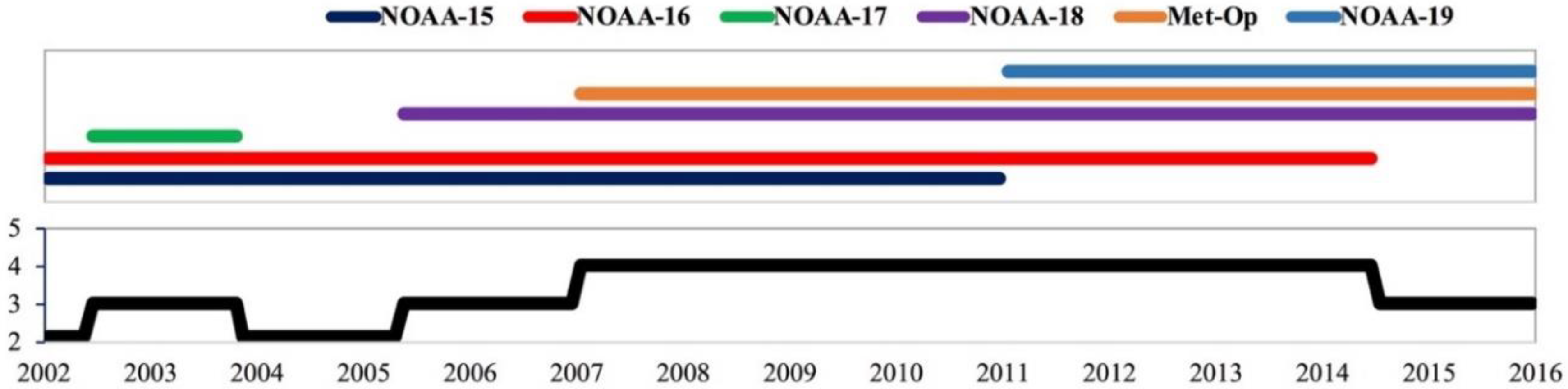
In this section, the general attributes of the HBC are evaluated through comparisons with other well-known data sets, such as satellite-derived products and model reanalysis. The primary purpose is to show where they are similar and different, and point out features that may be anomalous. In many instances, data from 2008 is used as a representative time period from the 16-year data set, because it is a period of multiple satellites in operation (refer to
Figure 2).
Two products are not shown in this manuscript—CLW and IWP. Due to the lack of comprehensive validation data for these products, as well as known uncertainties in reanalysis data sets like MERRA2, they may be less reliable and, therefore, comparisons are not presented.
3.1. Advantages and Disadvantages of the Hydrological Bundle
Some advantages of the HBC are that the AMSU/MHS microwave scan geometry offers a wider swath width than other microwave sensors, such as the SSM/I, thus, there are fewer orbital gaps and better coverage at the poles. In addition, the microwave sounder offers a complement of surface and atmospheric channels for both temperature and moisture. Finally, multiple satellites offer better diurnal cycle sampling, as shown in
Figure 1; after 2000, there are at least two satellites available, and up to four satellites from January 2007 to June 2014. The temporal sampling is roughly 4 h apart, allowing reasonable sampling of the diurnal cycle.
A disadvantage of the HBC is that, due to the microwave sounder cross-track scan geometry, the Earth incidence angle varies, which makes retrievals more difficult because of changes in atmospheric attenuation, surface emissivity, and lack of dual polarization. Also, although there is a wider swath width as compared to microwave imagers, the last few observations along the scan are approximately twice as large as at nadir, potentially providing degraded TCDR retrieval for small scale phenomena, like precipitation.
3.2. Precipitation
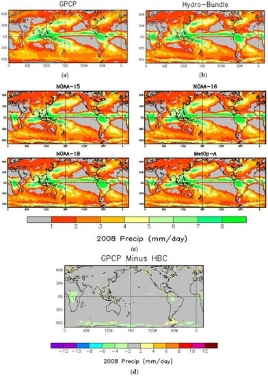
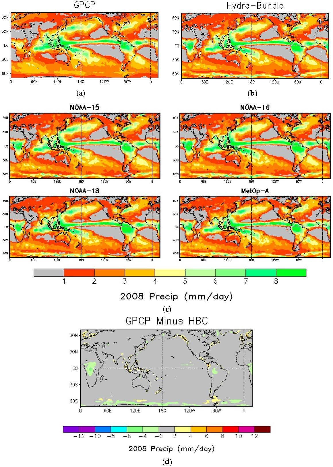
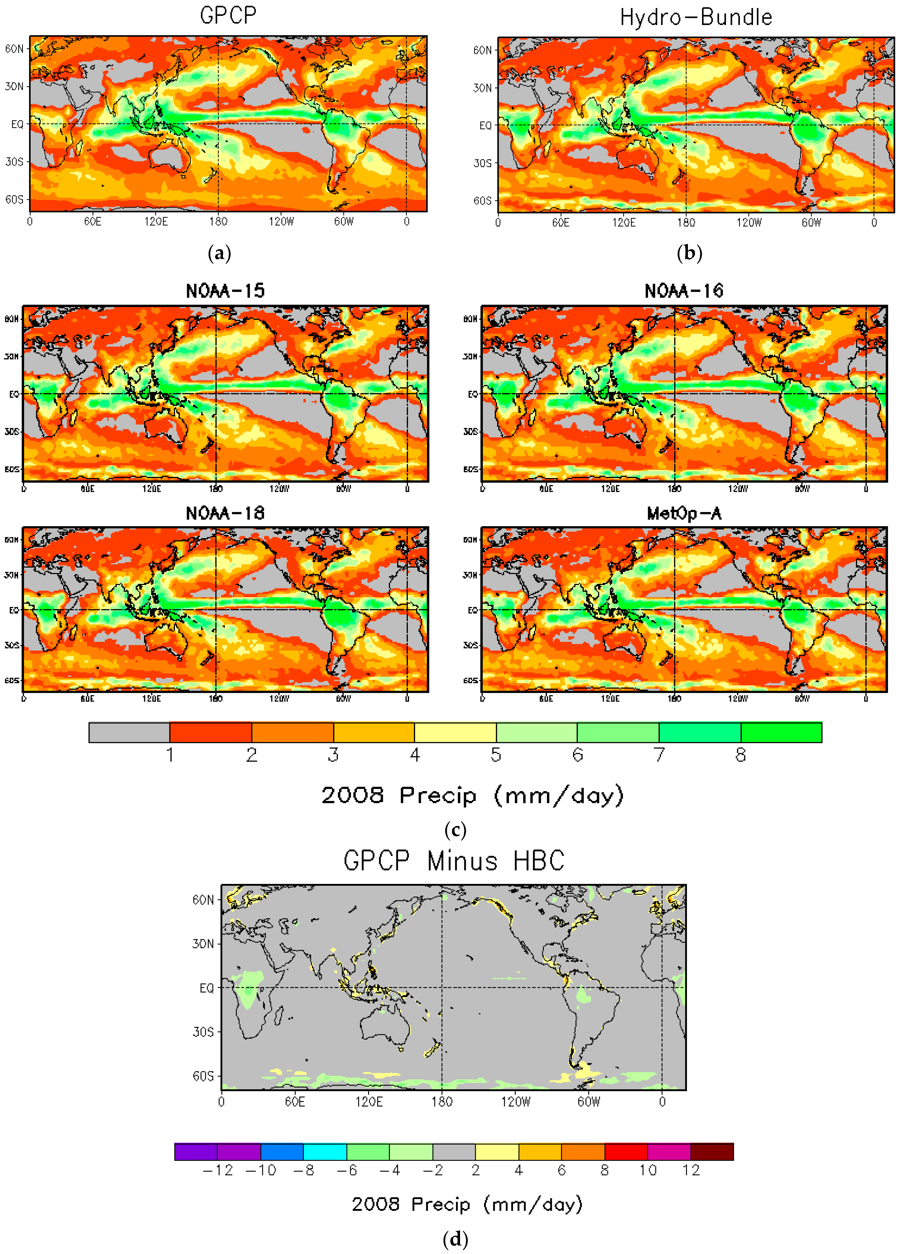
An examination of the annual precipitation averages for 2008 show good agreement between HBC (all available satellites) and GPCP (
Figure 3). Patterns of precipitation associated with the major precipitation belts across the globe match well, e.g., the intertropical convergence zone (ITCZ), south pacific convergence zone (SPCZ), mid-latitude ocean storm tracks, etc. There are some significant differences in magnitudes, most notably, higher values over tropical land regions in the HBC, which can be as large as 4 mm/day. This is a known positive bias with passive microwave land retrieval algorithms [
19]. Additional artifacts in the HBC appear to be associated with coastlines and sea-ice boundaries. This is most likely attributed to inadequacies of the coastline precipitation retrieval and sea-ice boundary delineation in MSPPS [
5]. A further breakdown by satellite shows no significant differences on the annual average for 2008, however, subtle features are noted in some land regions, presumably due to diurnal cycle differences.
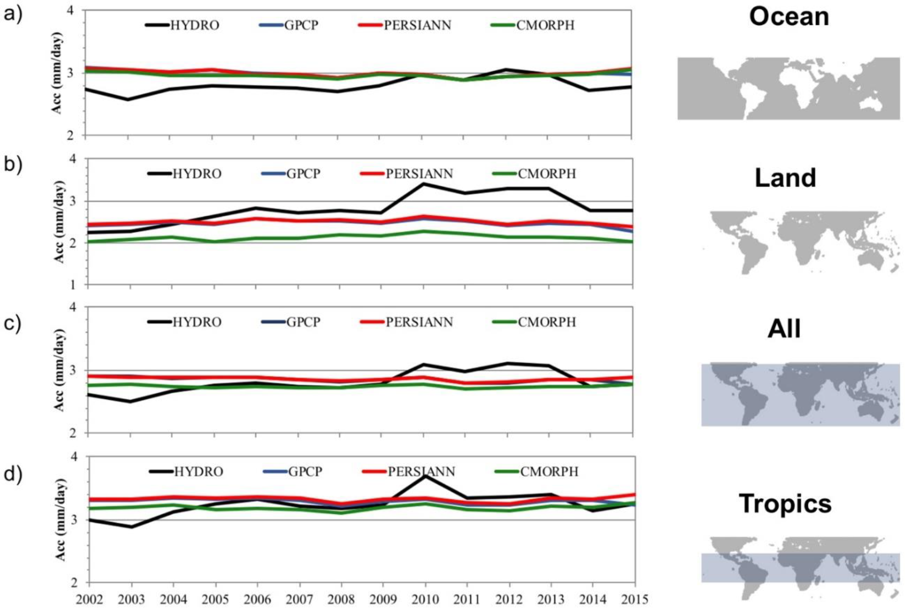
A quantitative comparison of the precipitation estimates derived from the HBC against the other satellite-based estimates is provided in
Figure 4. Comparisons are conducted for different areas; ocean (
Figure 4a), land (
Figure 4b), and all areas (
Figure 4c) between the latitudes 50°N and 50°S, and over the tropics, that is, between the latitudes 23°N and 23°S (
Figure 4d). Over oceans, HBC displays some differences with the other products, including a lower annual average than GPCP, PERSIANN, and CMORPH for the earlier part of the comparison (2002–2010,
Figure 4a). The fact that those three comparison satellite products are close over ocean is expected, due to the fact that both PERSIANN and CMORPH use GPCP for calibration. For the period (2010–2013), differences are less important, and HBC compares well with other estimates while displaying a lower annual average again for the later years (2014–2015). Over land, the differences are more pronounced. Precipitation estimates from HBC are close to GPCP and PERSIANN until 2010, but tend to be larger after 2010 and up to 2014. The differences observed are likely due to satellite intercalibration issues in the later part of the HBC time series. At the time of this writing, a new reference satellite is being tested for the FCDRs after 2010, and this will likely result in an improved time series when HBC Version 2 is completed. We remind the reader that HBC is a satellite-only product and, therefore, differences are expected from bias-adjusted satellite quantitative precipitation estimate (QPE). It is interesting to note that, while GPCP and PERSIANN remain close over land, due to the fact that PERSIANN uses GPCP for calibration, CMORPH, that uses in situ data for calibration over land, displays a lower average than the two other products. This indicates that even bias-adjusted products can have differences on the same order as the differences observed between the HBC and the bias-adjusted satellite QPEs (GPCP, PERSIANN, CMORPH). For all areas, 50°N–50°S comparisons are closer because land and ocean biases compensate each other (
Figure 4c). Important differences remain for 2010–2013, with a higher annual average rainfall indicated by HBC; some of this may be attributed to insufficient calibration information for the NOAA-16 satellite during the latter stages of its operation. Future versions of the HBC will account for this problematic data period. Finally, for the tropics (23°N–23°S), all products indicate quantitatively comparable values for the average annual rainfall, with HBC alternatively lower (earlier period: 2002–2004) and higher (later period: 2010–2013) than the other satellite products, although for the remaining years, HBC remains between the range of the three other gauge-corrected products (
Figure 4d).
3.3. Total Precipitable Water (TPW)
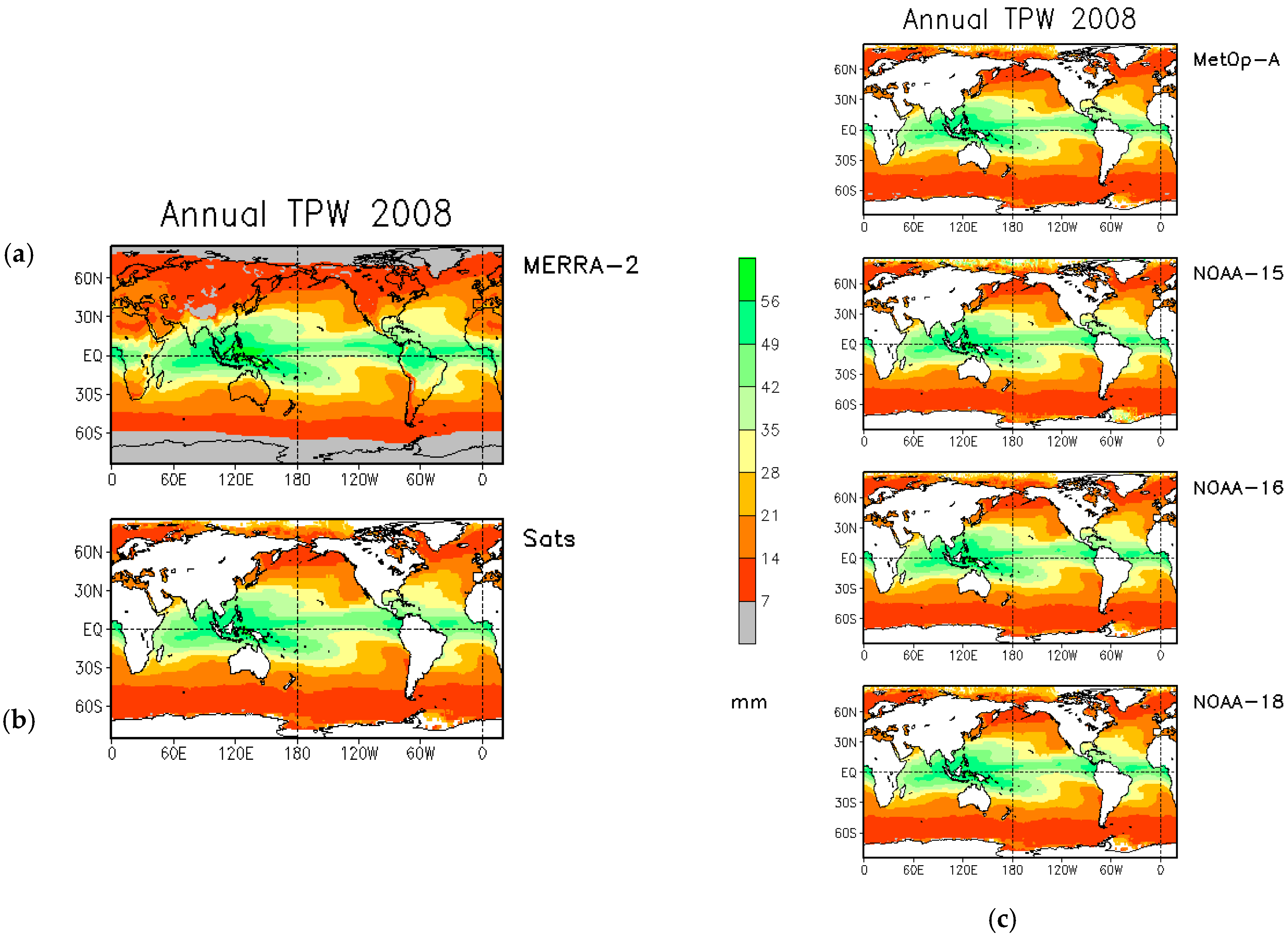
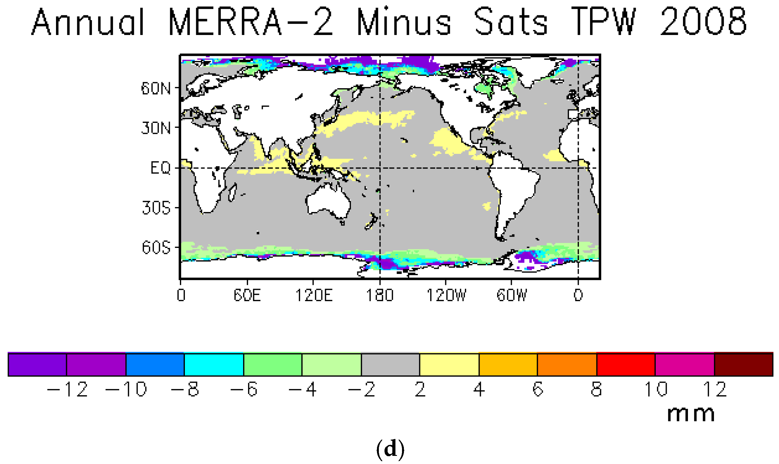
The TPW comparisons against MERRA-2 (
Figure 5) are similar to the precipitation comparisons in the sense that they are most alike in the mid and low latitudes, while the satellite estimate is higher over high latitudes. Note that the HBC TPW is for ocean only.
Features associated with the major circulation features are depicted similarly by both products, such as the maximums associated with the ITCZ and SPCZ, and the minimums in the subsidence zones that are found on the western zones off of many of the continental regions (e.g., North and South America and Africa). Breakdowns by each satellite show virtually no differences, as might be expected for TPW, which has little diurnal variability. There are two regions that have significant biases. The largest is evident in the polar regions, where the HBC is apparently contaminated by sea-ice, causing significant overestimates. The MERRA-2 has large areas of higher TPW than the HBC (on the order of 2 mm), which are mostly at the edges of transition zones of moist to dry environments associated with major atmospheric circulation regions. It is possible that the MERRA-2 has a smoother transition zone during some seasons than the HBC, and might be suspect in those regions.
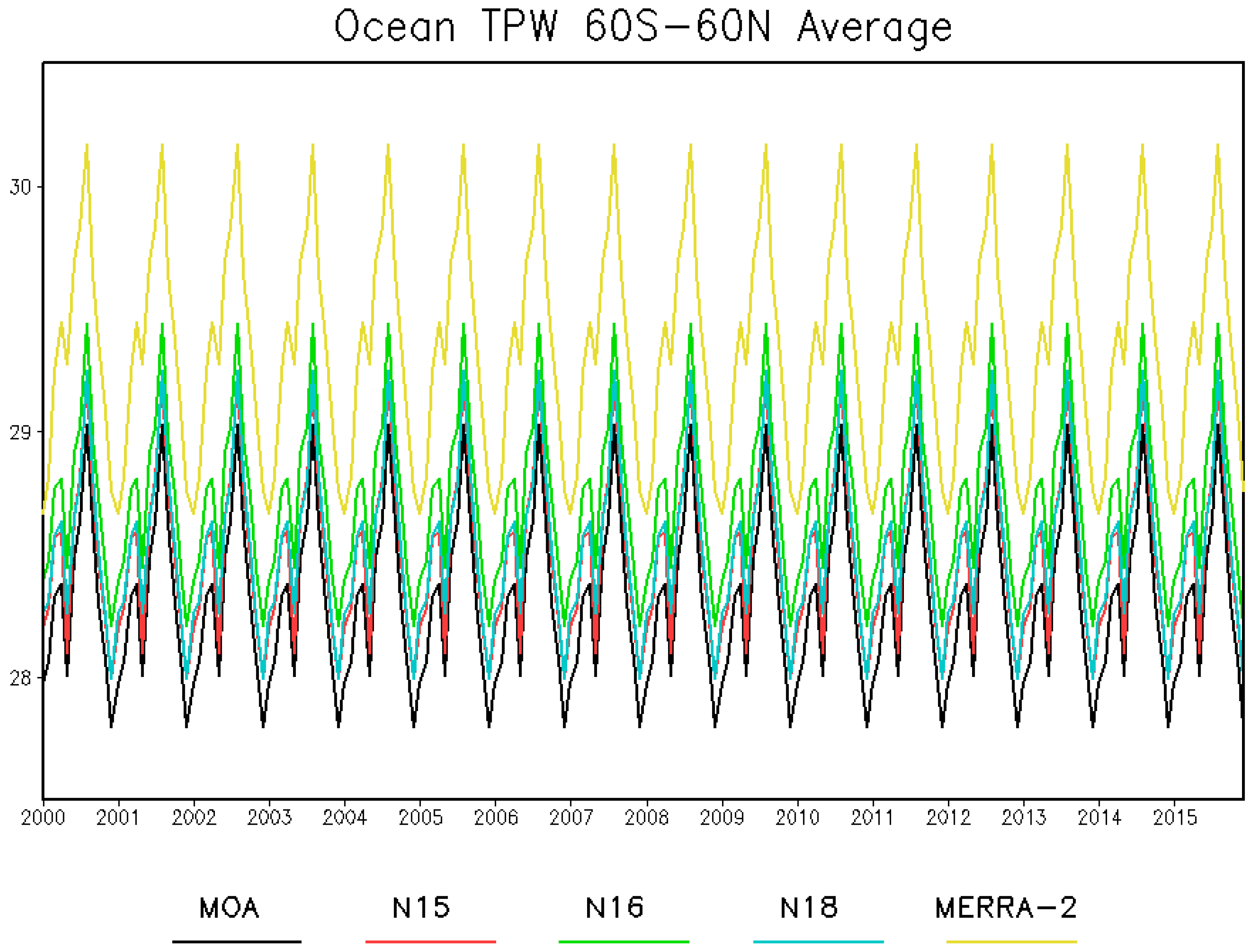
A closer look at the variations within the entire time series is shown in
Figure 6. Although the MERRA-2 shows higher values, the annual cycle for the 16-year period is similar for all satellites. As a testimony to the intercalibration within the FCDRs for AMSU-A, which is used in the TCDR for TPW, there is consistency between all of the satellites shown in
Figure 6.
3.4. Land Surface Temperature (LST)
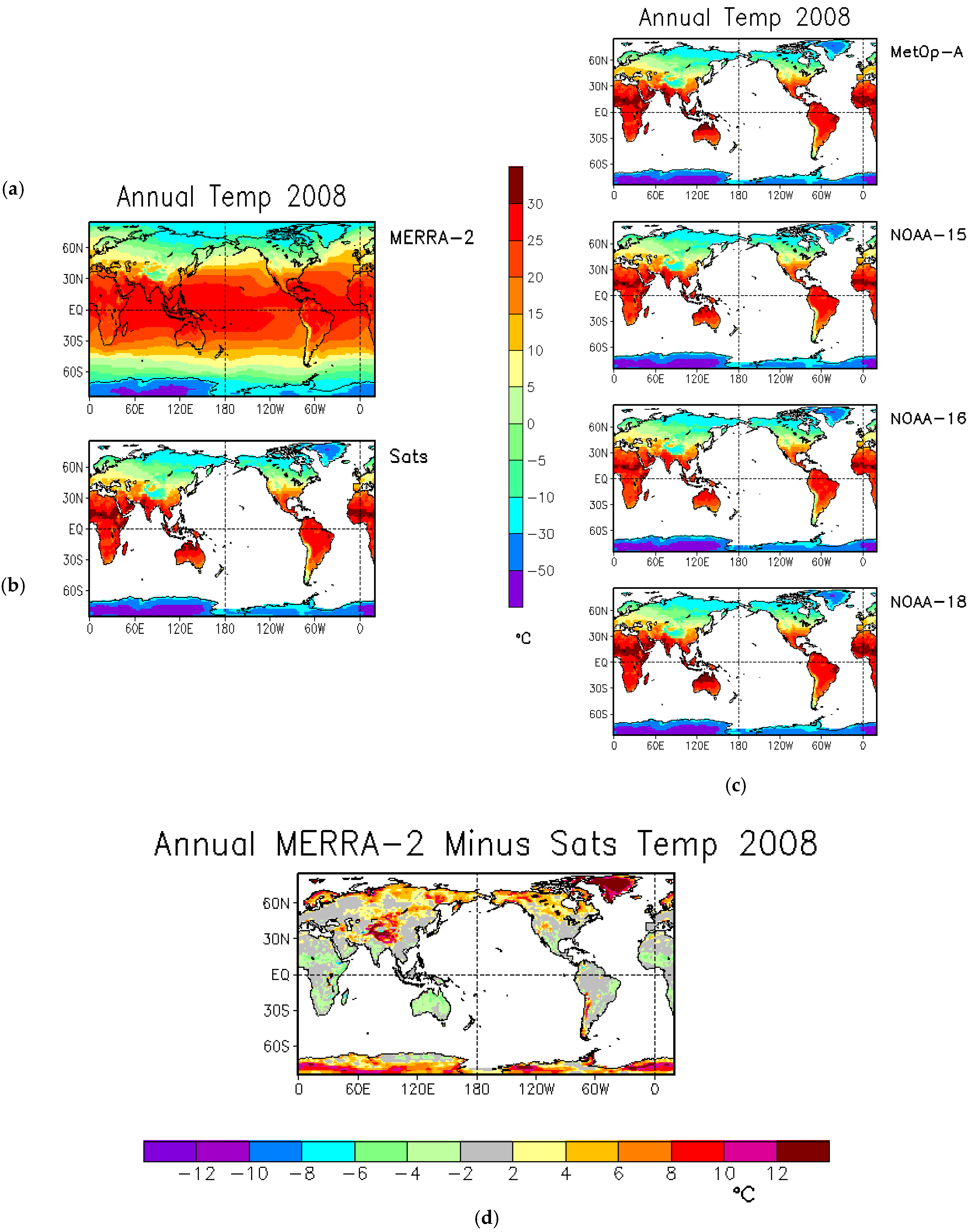
For land surface temperature (
Figure 7), the overall patterns between the HBC and MERRA-2 are similar. However, the satellite estimate is lower over high-altitude locations, including Antarctica, Greenland, and the Himalayas, which may be attributed to improper handling of the highly variable land emissivity over these complex surfaces in the MSPPS algorithm. The satellite estimates also tend to be cooler over much of the high latitude Northern Hemisphere land. MERRA-2 estimates are slightly cooler over much of the tropics. There are subtle differences between the four different satellites shown, and these are most likely explained by the overpass times of the different satellites (refer to
Figure 1). For example, NOAA-18 shows a broader area of higher temperatures in the tropical regions, because in 2008, the satellite observed these regions around 1400 local time, near the maximum diurnal cycle.
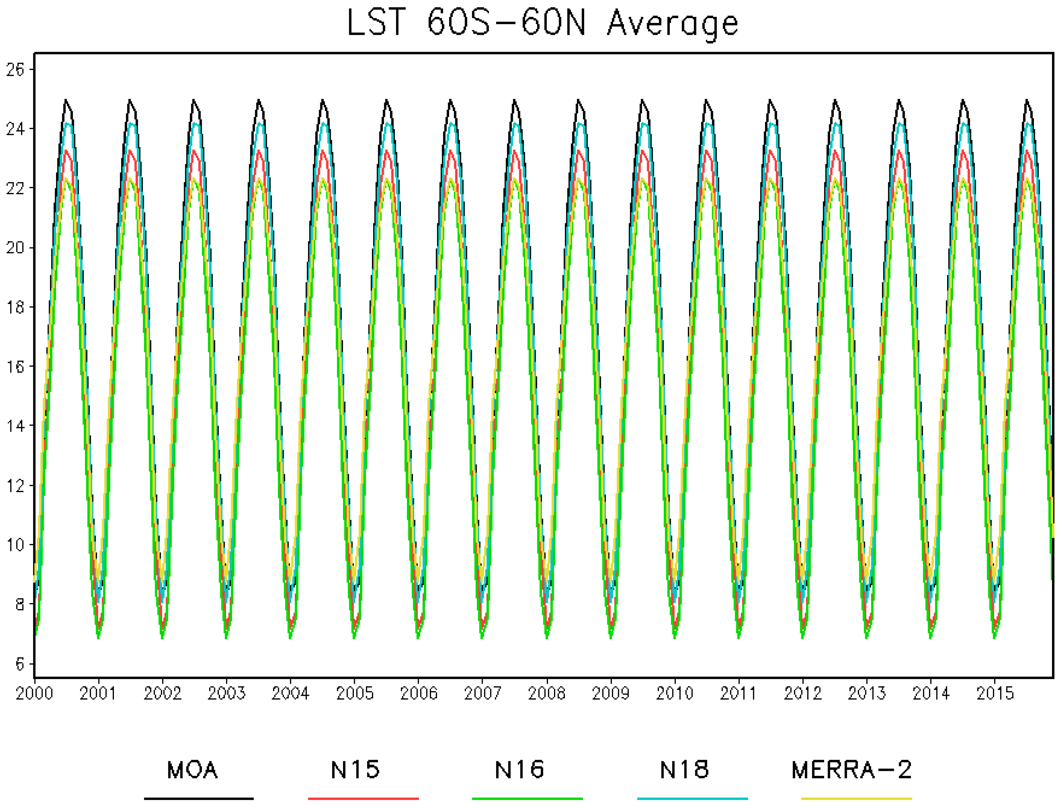
A closer look at the variations within the entire time series is shown in
Figure 8. All give the same LST annual cycle, but there are differences in the average and amplitude. Although the HBC inputs all have similar amplitudes, the MetOp satellite is warmest, and NOAA-16 is coolest, likely due to the sampling time of the day. The MERRA-2 estimate has smaller amplitude than the satellite estimates, perhaps because the satellite estimates are based on surface radiation, while the reanalysis estimate is from a near-surface model level. It is apparent, though, that none of the data sets show any distinct trend over the period of record.
3.5. Ice and Snow Cover
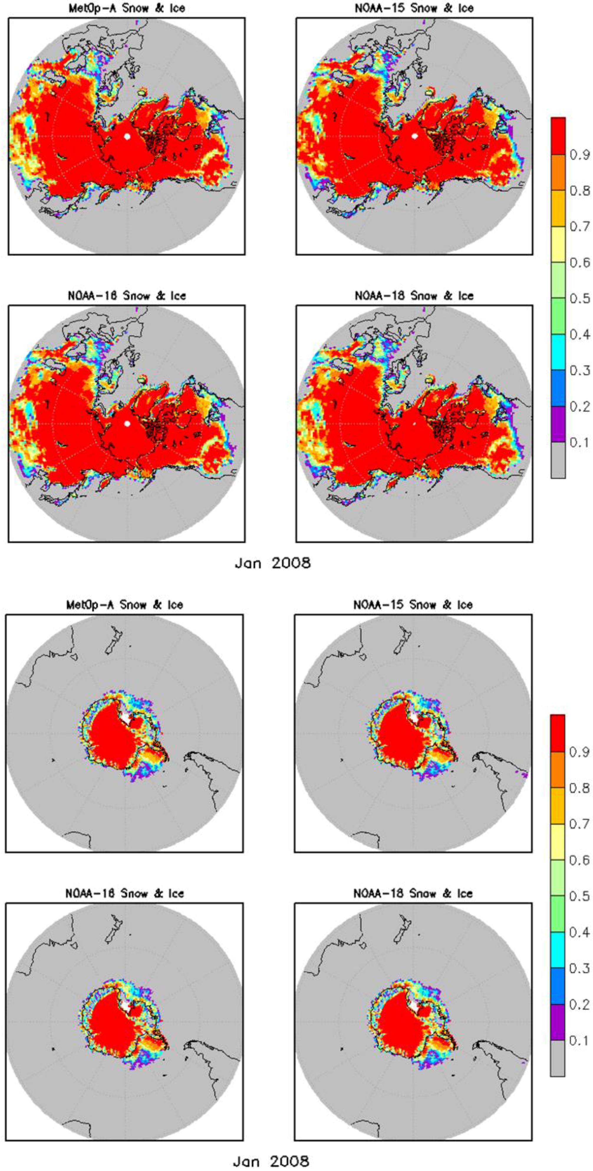
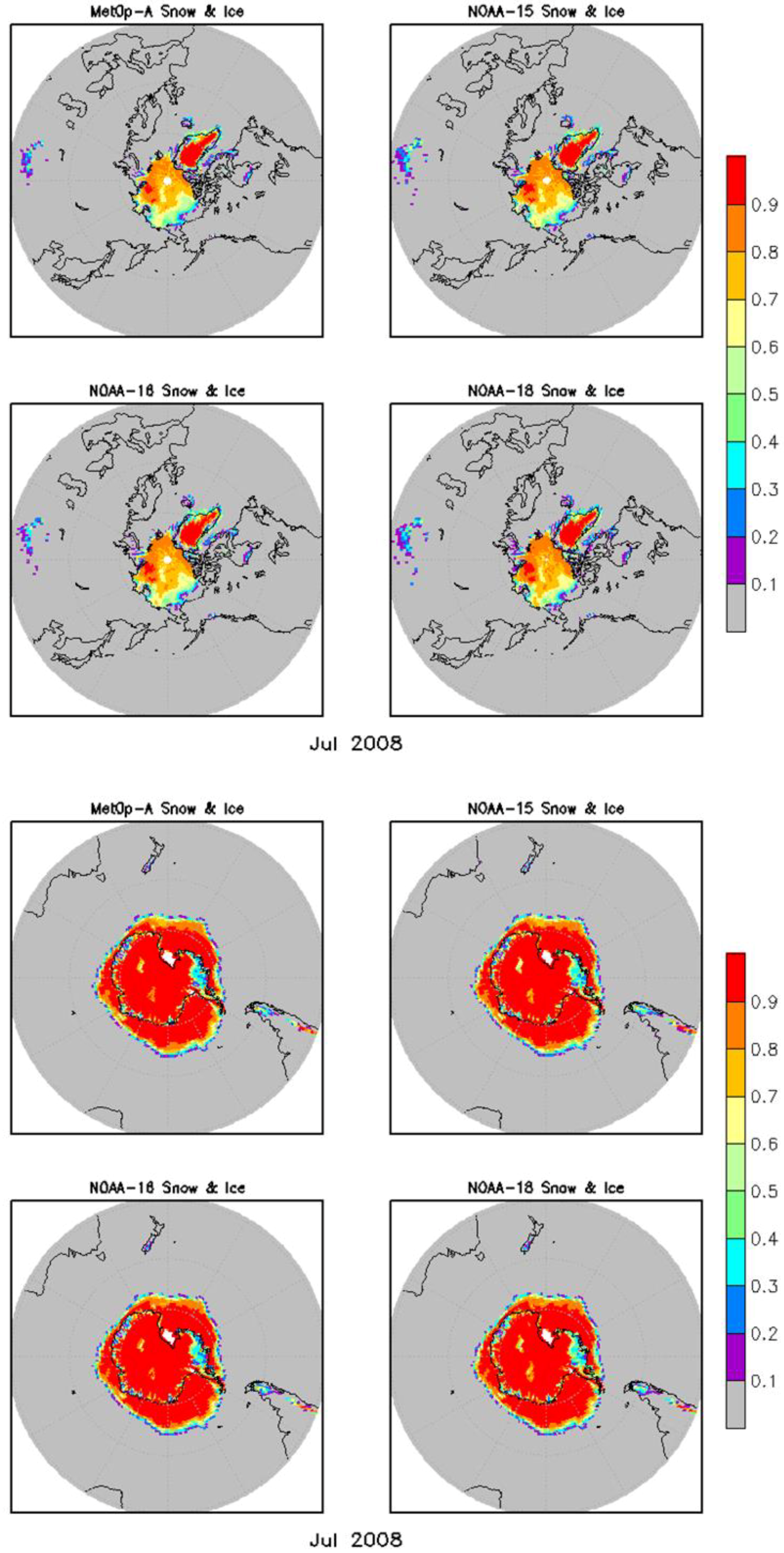
Satellite estimates of combined snow and ice fraction are shown for January 2008 (
Figure 9) and July 2008 (
Figure 10). The different satellite estimates for these months are nearly the same. Comparison of January and July shows the annual cycle of ice concentration and fractional snow cover. The greatest seasonal variation is over the Northern Hemisphere, where the larger land area shows great contrast from the cool to warm months, and where the polar ocean also indicates large changes in ice concentration.
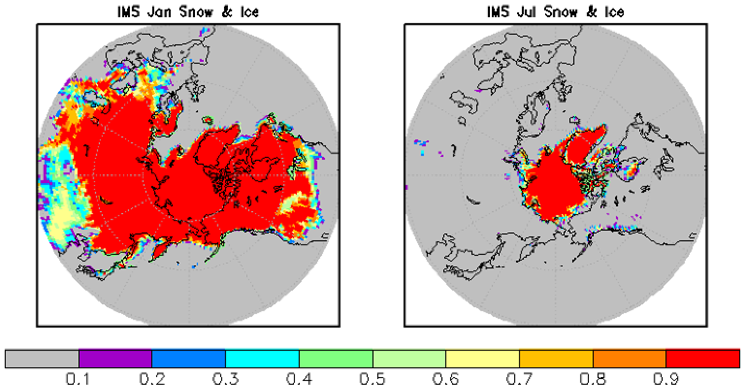
For the Northern Hemisphere, the IMS snow and sea-ice estimates are available for comparison. Each daily IMS estimate is either land with no snow, land with snow, sea with no ice, or sea-ice. The daily IMS snow and ice estimates are gridded to a 1° grid, and at each grid square, the fraction of the available estimates in the square with snow or ice is computed. Then, the monthly fraction of each is computed for 1999 to 2017. Maps for January and July 2008 (
Figure 11) are shown for comparison to the various satellite map estimates for January and July 2008. The IMS land snow-cover maps are similar to the satellite estimates. However, the IMS sea-ice fractional estimate is systematically higher than the satellite estimates in the warm season, when the IMS estimate tends to be near 1 in many areas. Some of the lower fraction in the satellite estimates may be due to interpretation of fresh-water ice ponds on top of the ice as open water, lowering the fraction estimate, whereas the IMS, with a human analyst making a final decision, is able to delineate these regions by using other satellite products, such as visible imagery.
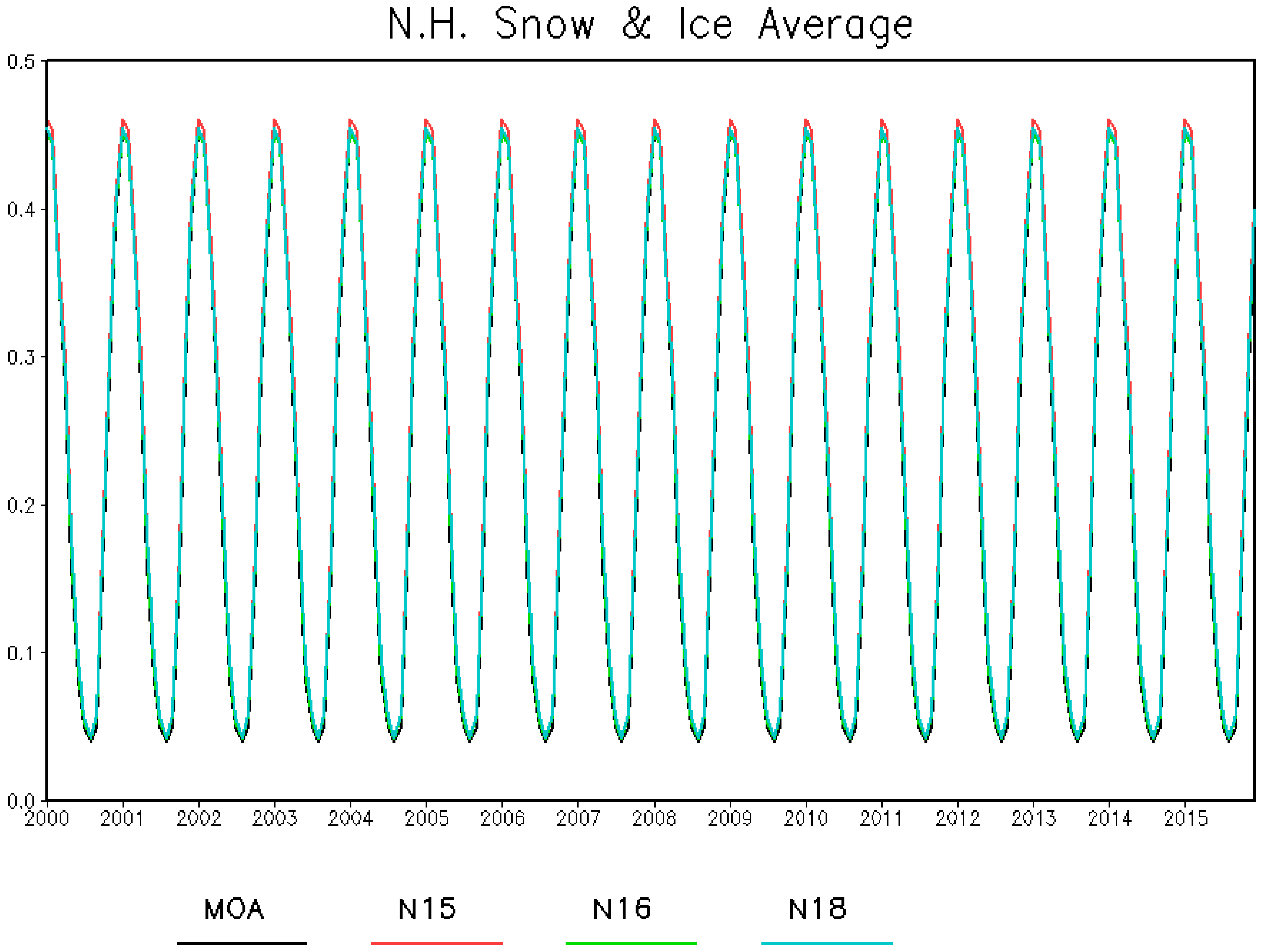
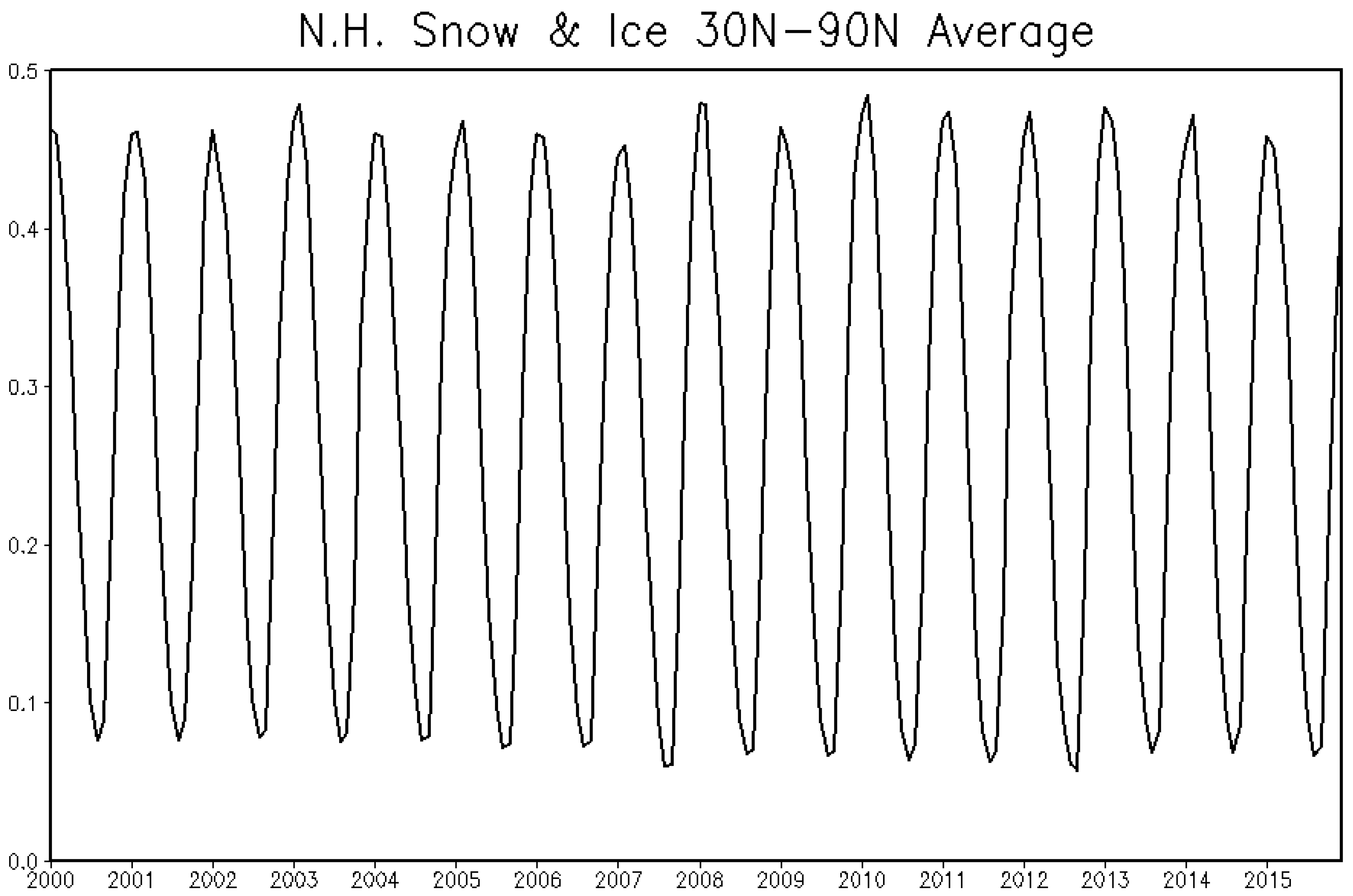
A final comparison of the snow and ice is a time series over the 16-year period. These are shown in
Figure 12, where each individual satellite (top) and the IMS (bottom) are shown. The satellite estimates are extremely consistent among themselves, and from year to year. On the other hand, the IMS shows variations between minimum and maximum for some years.
4. Conclusions
The AMSU/MHS hydrological bundle TCDR provides vital information on several key variables, including precipitation, water vapor, snow cover, and sea-ice, which are critical components of the Earth’s hydrological cycle. There are several important attributes of the HBC that make it unique from other similar data sets. First, the majority of this sixteen-year data set contains measurements from different times of the day and, therefore, the diurnal cycle can be captured. This is because the NOAA and MetOp satellites are critical components of the global passive microwave constellation and, by design, are operated as a three-satellite configuration, making measurements approximately four hours apart. Secondly, as we have demonstrated, the HBC product quality is comparable to other data sets that have been derived from satellites, in situ data, dynamic reanalyses, or their combinations. The user community can exploit these data to supplement other existing data sets, and be confident of general consistency, with a few caveats noted in the paper (e.g., biased regions, such as over sea-ice, high elevation surfaces, coastlines, etc.) Finally, the HBC is one of the few satellite TCDRs that are part of NOAA’s/NCEI’s operational production suite, thereby adhering to the strict standards of NOAA’s CDR program and transition to operation procedures. Their production is, therefore, transparent in nature and reproducible by other groups, because all of the methodologies employed are properly documented.
In the future, the HBC will continue to expand to other years through the lifespan of the NOAA and MetOp satellites containing AMSU-A and MHS sensors. The data set producers further hope to continue the time series with newer sensors that replace the AMSU/MHS sensors, such as the Advanced Technology Microwave Sounder (ATMS) on board the NOAA/JPSS satellites, and the Microwave Sounder (MWS) on board the EUMETSAT polar system Second Generation (EPS-SG).
Author Contributions
R.F. is currently the principal investigator for the HBC and led the writing of the paper. B.N. is the NOAA archive focal point for the HBC and suggested contributing this paper to the Remote Sensing special issue. T.S. and O.P. generated the majority of the figures and contributed to the analysis of the products. All authors discussed the results presented in this paper.
Funding
The majority of the funding for this project has been provided by the NOAA, National Centers for Environmental Information.
Acknowledgments
We would like to thank the efforts of H. Meng, W. Yang, I. Moradi, J. Beauchamp and Y. You of NOAA and the NOAA Cooperative Institute for Climate and Satellites (CICS) at the University of Maryland for the generation of the CDR’s. We also want to thank H.-T. Lee, also of CICS, for supplying
Figure 1.
Conflicts of Interest
The authors declare no conflict of interest. The views, opinions, and findings contained in this report are those of the author(s) and should not be construed as an official National Oceanic and Atmospheric Administration or U.S. Government position, policy, or decision.
References
- Wilheit, T.T.; Chang, A.T.C.; Rao, M.S.V.; Rodgers, E.B.; Theon, J.S. A satellite technique for quantitatively mapping rainfall rates over the ocean. J. Appl. Meteor 1977, 16, 551–560. [Google Scholar] [CrossRef]
- Wilheit, T.T.; Chang, A.T.C. An algorithm for retrieval of ocean surface and atmospheric parameters from the observations of the scanning multichannel microwave radiometer. Radio Sci. 1980, 15, 525–544. [Google Scholar] [CrossRef]
- Yang, W.; Meng, H.; Ferraro, R.; Moradi, I.; Divaraj, C. Cross scan asymmetry of AMSU-A window channels: Characterization, correction and verification. IEEE Trans. Geosci. Remote. Sens. 2013, 51, 1514–1530. [Google Scholar] [CrossRef]
- Moradi, I.; Buehler, S.; John, V.; Reale, A.; Ferraro, R. Evaluating instrumental inhomogeneities in global radiosonde upper tropospheric humidity data using microwave satellite data. IEEE Trans. Geosci. Remote. Sens. 2013, 51, 3615–3624. [Google Scholar] [CrossRef]
- Ferraro, R.R.; Weng, F.; Grody, N.; Zhao, L.; Meng, H.; Kongoli, C.; Pellegrino, P.; Qiu, S.; Dean, C. NOAA operational hydrological products derived from the AMSU. IEEE Trans. Geosci. Remote. Sens. 2005, 43, 1036–1049. [Google Scholar] [CrossRef]
- Kidwell, K.B. NOAA Polar Orbiter Data (TIROS-N, NOAA-6, NOAA-7, NOAA-8, NOAA-9, NOAA-10, NOAA-11, And NOAA-12) Users Guide; National Oceanic and Atmospheric Administration, National Environmental Satellite, Data, and Information Service, National Climatic Data Center, Satellite Data Services Division: Washington, DC, USA, 1991.
- Robel, J.; Graumann, A.; Kidwell, K.; Aleman, R.; Ruff, I.; Muckle, B.; Kleespies, T. NOAA KLM User’s Guide, with NOAA-N, N Prime and MetOp Supplements, Users Guide; National Oceanic and Atmospheric Administration, National Environmental Satellite, Data, and Information Service, National Climatic Data Center, Remote Sensing and Applications Division: Asheville, NC, USA, 2014.
- Ferraro, R.R.; Weng, F.; Grody, N.C.; Basist, A. An eight year (1987–1994) climatology of rainfall, clouds, water vapor, snowcover, and sea-ice derived from SSM/I measurements. Bull. Am. Meteor Soc. 1996, 77, 894–905. [Google Scholar] [CrossRef]
- Sapiano, M.R.P.; Berg, W.K.; McKague, D.S.; Kummerow, C.D. Toward an intercalibrated fundamental climate data record of the SSM/I sensors. IEEE Trans. Geosci. Remote. Sens. 2013, 51, 1492–1503. [Google Scholar] [CrossRef]
- Vila, D.; Ferraro, R.; Hernandez, C.; Semunegus, H. The performance of hydrological monthly products using SSM/I—SSMI/S sensors. J. Hydromet. 2013, 14, 266–274. [Google Scholar] [CrossRef]
- Huffman, G.J.; Adler, R.F.; Morrissey, M.; Bolvin, D.; Curtis, S.; Joyce, R.; McGavock, B.; Susskind, J. Global precipitation at one-degree daily resolution from multi-satellite observations. J. Hydrometeorol. 2001, 2, 36–50. [Google Scholar] [CrossRef]
- Schneider, U.; Becker, A.; Finger, P.; Meyer-Christoffer, A.; Ziese, M.; Rudolf, B. GPCC’s new land surface precipitation climatology based on quality-controlled in situ data and its role in quantifying the global water cycle. Theor. Appl. Climatol. 2014, 115, 15–40. [Google Scholar] [CrossRef]
- Gelaro, R.; McCarty, W.; Suárez, M.J.; Todling, R.; Molod, A.; Takacs, L.; Randles, C.A.; Darmenov, A.; Bosilovich, M.G.; Reichle, R.; et al. The Modern-Era Retrospective Analysis for Research and Applications, Version 2 (MERRA-2). J. Clim. 2017, 30, 5419–5454. [Google Scholar] [CrossRef]
- Bosilovich, M.G.; Robertson, F.R.; Takacs, L.; Molod, A.; Mocko, D. Atmospheric water balance and variability in the MERRA-2 Reanalysis. J. Clim. 2007, 30, 1177–1196. [Google Scholar] [CrossRef]
- Joyce, R.; Janowiak, J.; Arkin, P.; Xie, P. CMORPH: A method that produces global precipitation estimates from passive microwave and infrared data at high spatial and temporal resolution. J. Hydrometeorol. 2004, 5, 487–503. [Google Scholar] [CrossRef]
- Xie, P.; Joyce, R.; Wu, S.; Yoo, S.-H.; Yarosh, Y.; Sun, F.; Lin, R. Reprocessed, bias-corrected CMORPH global high-resolution precipitation estimates from 1998. J. Hydrometeorol. 2017, 18, 1617–1641. [Google Scholar] [CrossRef]
- Ashouri, H.; Hsu, K.; Sorooshian, S.; Braithwaite, D.; Knapp, K.R.; Cecil, L.D.; Nelson, B.R.; Prat, O.P. PERSIANN-CDR: Daily precipitation climate data record from multi-satellite observations for hydrological and climate studies. Bull. Am. Meteor Soc. 2015, 96, 69–80. [Google Scholar] [CrossRef]
- Ramsay, B.H. The interactive multisensor snow and ice mapping system. Hydrol. Process. 1998, 12, 1537–1546. [Google Scholar] [CrossRef]
- McCollum, J.R.; Gruber, A.; Ba, M.B. Discrepancy between gauges and satellite estimates of rainfall in equatorial Africa. J. Appl. Meteor Clim. 2000, 39, 666–679. [Google Scholar] [CrossRef]
Figure 1.
Local time of ascending node for NOAA and MetOp satellites from 1979 through 2016. The number represents the satellite name (e.g., 5 = NOAA-5; 19 = NOAA-19; 20 = MetOp-A; and 21 = MetOp-B). The period of the hydrological bundle CDR (HBC) is shaded in yellow.
Figure 1.
Local time of ascending node for NOAA and MetOp satellites from 1979 through 2016. The number represents the satellite name (e.g., 5 = NOAA-5; 19 = NOAA-19; 20 = MetOp-A; and 21 = MetOp-B). The period of the hydrological bundle CDR (HBC) is shaded in yellow.
Figure 2.
Temporal period for each satellite and the corresponding number of satellites for the period 2002 to 2016, when at least three satellites were in operation.
Figure 2.
Temporal period for each satellite and the corresponding number of satellites for the period 2002 to 2016, when at least three satellites were in operation.
Figure 3.
Daily average precipitation for 2008 for (a) GPCP, and (b) hydrological bundle, and (c) daily average precipitation for 2008 for each satellite. GPCP minus HBC (all satellites) is shown in (d).
Figure 3.
Daily average precipitation for 2008 for (a) GPCP, and (b) hydrological bundle, and (c) daily average precipitation for 2008 for each satellite. GPCP minus HBC (all satellites) is shown in (d).
Figure 4.
Comparison of average annual precipitation for the HBC and other gridded satellite products of the CDR program (GPCP, PERSIANN, CMORPH). Comparisons are conducted for the band 50°N–50°S: (a) over ocean, (b) over land, (c) globally, and (d) for the tropics 23°N–23°S.
Figure 4.
Comparison of average annual precipitation for the HBC and other gridded satellite products of the CDR program (GPCP, PERSIANN, CMORPH). Comparisons are conducted for the band 50°N–50°S: (a) over ocean, (b) over land, (c) globally, and (d) for the tropics 23°N–23°S.
Figure 5.
Annual total precipitable water for 2008 for MERRA-2 (a), HBC—all satellites (b), each individual satellite (c), and MERRA—minus all satellites (d).
Figure 5.
Annual total precipitable water for 2008 for MERRA-2 (a), HBC—all satellites (b), each individual satellite (c), and MERRA—minus all satellites (d).
Figure 6.
Time series of monthly mean TPW (mm) for each satellite in the HBC and MERRA-2 for the band between 60°S and 60°N.
Figure 6.
Time series of monthly mean TPW (mm) for each satellite in the HBC and MERRA-2 for the band between 60°S and 60°N.
Figure 7.
Annual surface temperature for 2008 for MERRA-2 (a), HBC—all satellites (b), each individual satellite (c), and mERRA—Minus all satellites (d).
Figure 7.
Annual surface temperature for 2008 for MERRA-2 (a), HBC—all satellites (b), each individual satellite (c), and mERRA—Minus all satellites (d).
Figure 8.
Time series of monthly mean LST (deg C) for each satellite in the HBC and MERRA-2 for the band between 60°S and 60°N.
Figure 8.
Time series of monthly mean LST (deg C) for each satellite in the HBC and MERRA-2 for the band between 60°S and 60°N.
Figure 9.
Monthly hemispheric snow cover (fraction of time with snow cover) and sea-ice concentration (monthly mean fractional coverage) for January 2008 for the Northern (upper) and Southern Hemispheres (lower), for N15, N16, N18, and MetOp-A.
Figure 9.
Monthly hemispheric snow cover (fraction of time with snow cover) and sea-ice concentration (monthly mean fractional coverage) for January 2008 for the Northern (upper) and Southern Hemispheres (lower), for N15, N16, N18, and MetOp-A.
Figure 10.
As in
Figure 9, but for July 2008.
Figure 10.
As in
Figure 9, but for July 2008.
Figure 11.
Northern Hemisphere combined monthly fraction of snow and sea-ice from the IMS analysis averaged to a 1° spatial grid for January 2008 (left) and July 2008 (right).
Figure 11.
Northern Hemisphere combined monthly fraction of snow and sea-ice from the IMS analysis averaged to a 1° spatial grid for January 2008 (left) and July 2008 (right).
Figure 12.
Time series of the mean 30°N–90°N average monthly combined snow and ice fraction from the indicated satellites (upper) and the IMS analysis (lower).
Figure 12.
Time series of the mean 30°N–90°N average monthly combined snow and ice fraction from the indicated satellites (upper) and the IMS analysis (lower).
Table 1.
AMSU-A/B/MHS L2 product attributes. Products listed include total precipitable water (TPW), cloud liquid water (CLW), sea-ice concentration (SIC), land surface temperature (LST), land surface emissivity (LSE), rain rate (RR), snow cover (SC), ice water path (IWP), and snow water equivalent (SWE).
| Parameter | Attribute |
|---|
| Satellite/Period of Record | NOAA-15: 1 January 2000–31 December 2016 |
| NOAA-16: 1 January 2000–9 June 2014 |
| NOAA-17: 25 June 2002–31 October 2003 |
| NOAA-18: 25 May 2005–31 December 2016 |
| NOAA-19: 11 February 2009–31 December 2016 |
| MetOp-A: 1 January 2007–31 December 2016 |
| Geographic Coverage | Global (2343 km swath width) |
| Spatial Resolution | 16 × 16 km (AMSU-A), 48 × 48 km AMSU-B/MHS at nadir |
| AMSU-A derived products | TPW, CLW, SIC, LST, LSE |
| AMSU-B/MHS derived products | RR, SC, IWP, SWE |
| Precision & Accuracy | Varies with product |
Table 2.
List of best times to use the various satellite products.
Table 2.
List of best times to use the various satellite products.
| | Best Times to Use | Comments |
|---|
| Satellite | AMSU-A TCDR (TPW, CLW, Sea-Ice, LST) | AMSU-B/MHS (IWP, RR, Snow) | AMSU-A | AMSU-B |
| N15 | January 2000–December 2016 | January 2000–December 2010 | Missing data periods in 2012 & 2014 | Missing data periods in 2012 & 2014 |
| N16 | January 2000–December 2016 | January 2000–December 2010 | | |
| N17 | Jul 2002–October 2003 | January 2002–October 2003 | | |
| N18 | Jun 2005–December 2016 | Jun 2005–December 2016 | | |
| N19 | Mar 2009–December 2016 | None | | NOAA sounding data FCDR so we do not generate TCDR |
| MOA | January 2007–December 2016 | | Missing data May and September 2012 | Missing data May and September 2012; May 2014 |
Table 3.
AMSU-A/B/MHS L2 suite of products.
Table 3.
AMSU-A/B/MHS L2 suite of products.
| Products | Units | Surface Type |
|---|
| Total Precipitable Water (TPW) | mm | Ocean |
| Cloud Liquid Water (CLW) | mm | Ocean |
| Cloud Liquid Water Frequency (CLF) | % | Ocean |
| Rain Rate (RR) | mm/h | Land and Ocean |
| Rain Frequency | % | Land and Ocean |
| Ice Water Path (IWP) | mm | Land and Ocean |
| Ice Water Path Frequency (IWF) | % | Land and Ocean |
| Snow Cover | Yes/No | Land |
| Surface Temperature | K | Land |
| Sea-Ice Concentration | % | Ocean |
© 2018 by the authors. Licensee MDPI, Basel, Switzerland. This article is an open access article distributed under the terms and conditions of the Creative Commons Attribution (CC BY) license (http://creativecommons.org/licenses/by/4.0/).


