Geospatial Analysis of Horizontal and Vertical Urban Expansion Using Multi-Spatial Resolution Data: A Case Study of Surabaya, Indonesia

 ,
,  ,
,  ,
, 

Abstract
:
1. Introduction
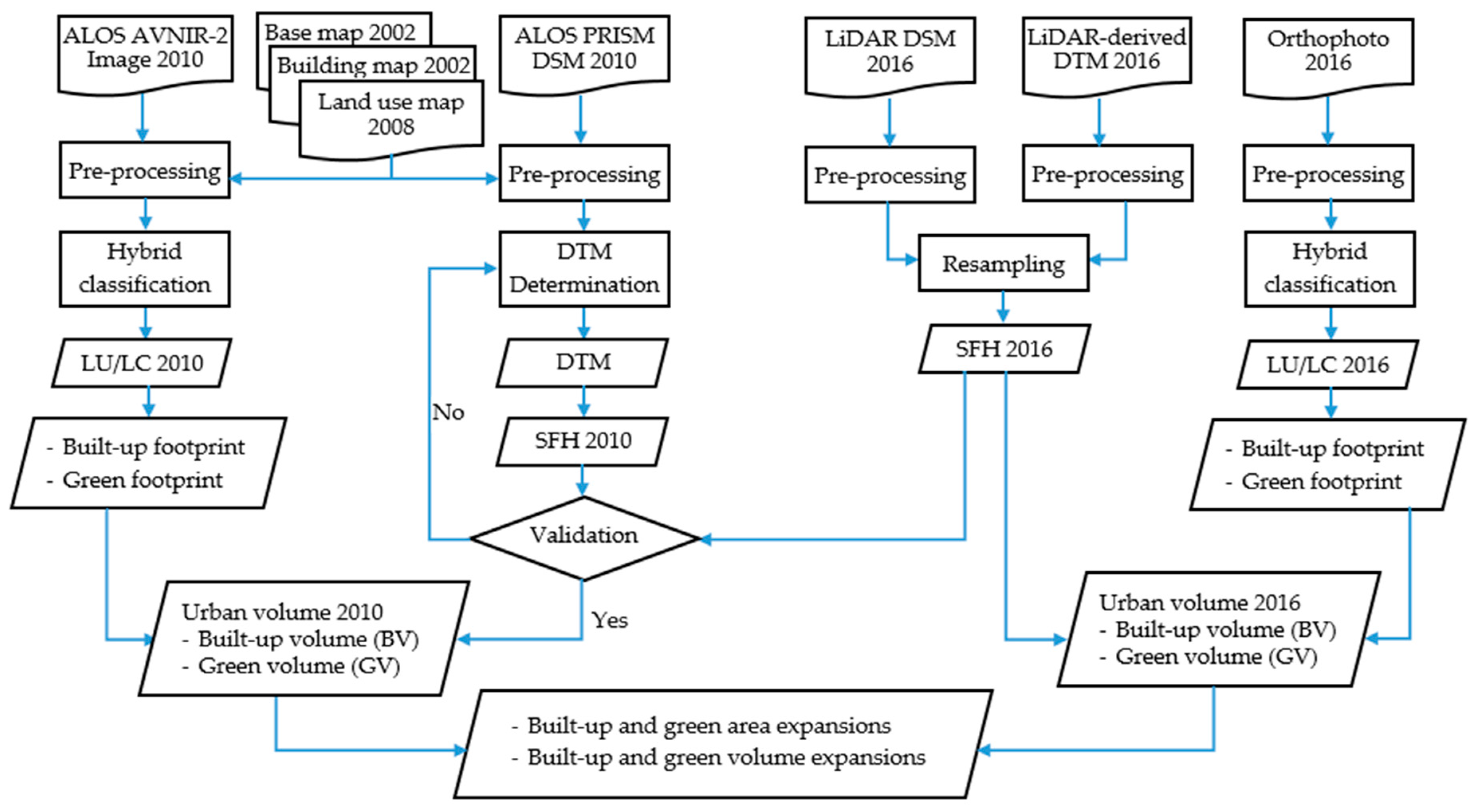
2. Methodology
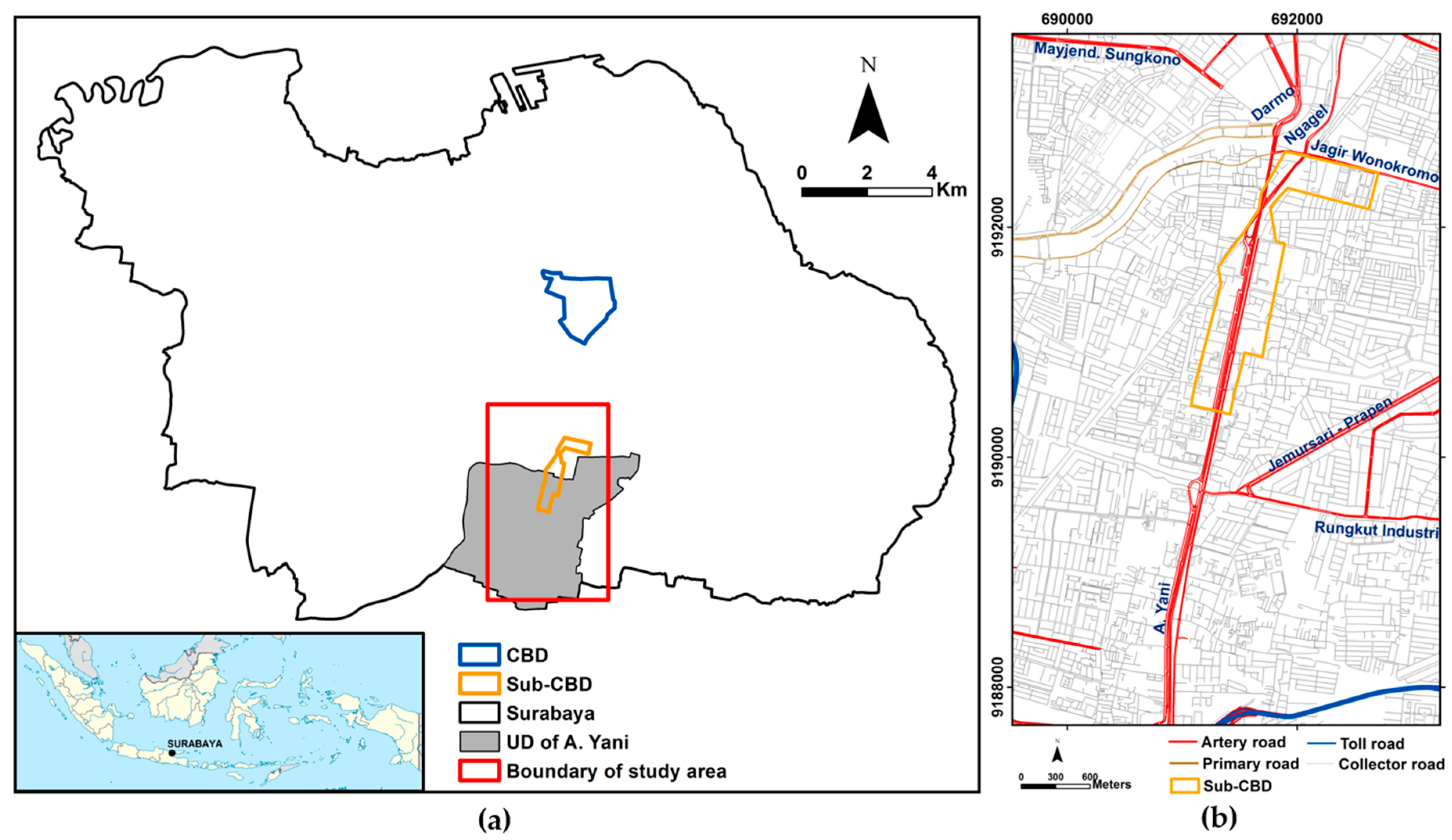
2.1. Study Area and Data Used
2.2. Land Use/Land Cover (LU/LC)
2.2.1. LU/LC of ALOS Image 2010
2.2.2. LU/LC of Orthophoto 2016
2.3. Urban Volume
2.3.1. DTM and Surface Feature Height (SFH) Determination
2.3.2. Validation of SFH
2.3.3. Built-Up and Green Volume
2.4. Built-Up and Green Expansions
2.4.1. Patch Metrics of Built-Up and Green Area
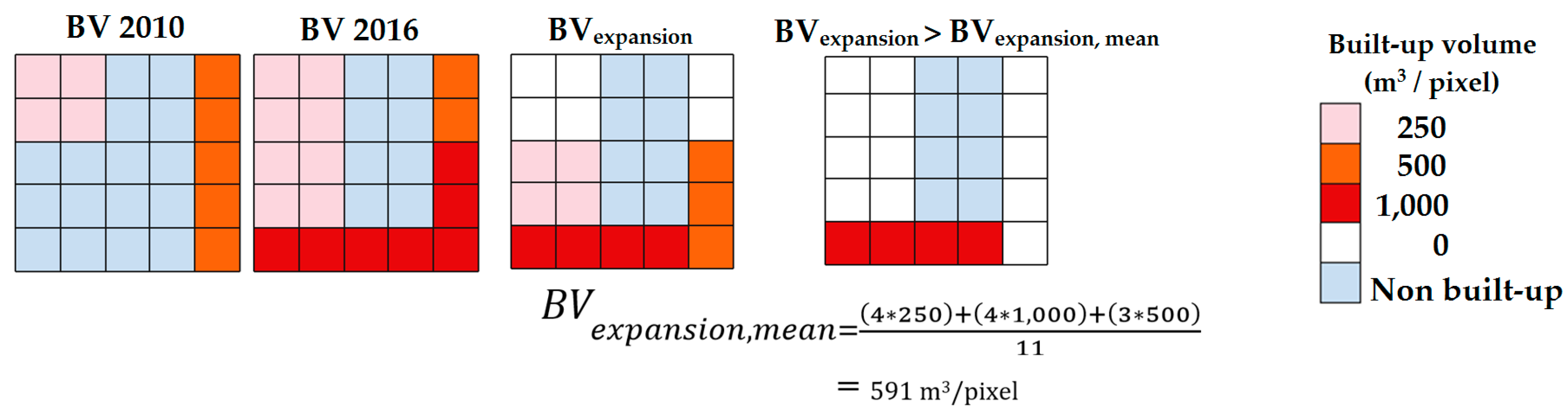
2.4.2. Built-Up and Green Volume Expansion Rates
3. Results
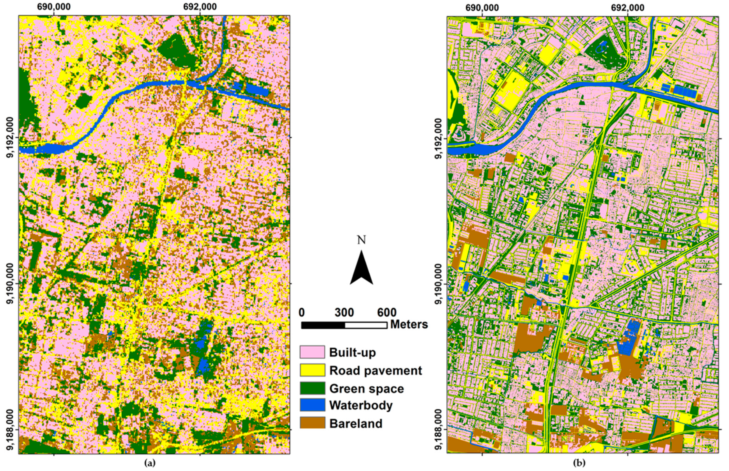
3.1. Land Use/Land Cover (LU/LC)
3.2. Urban Volume
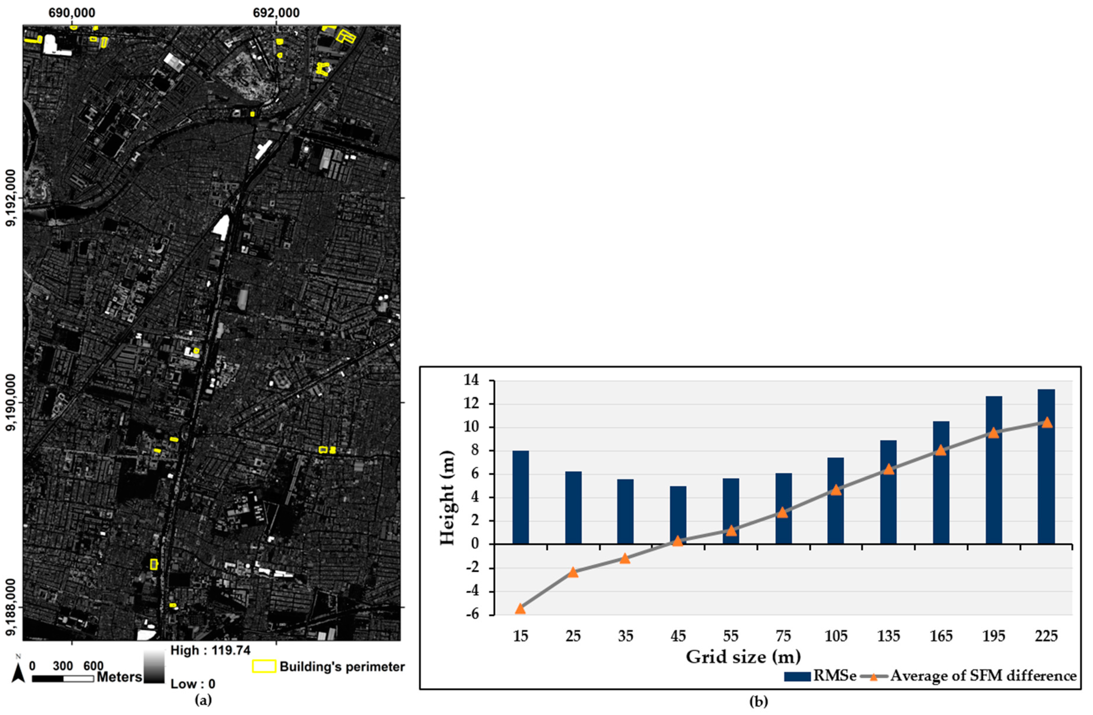
3.2.1. DTM and SFH Determination
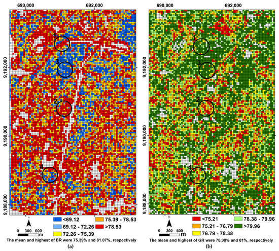
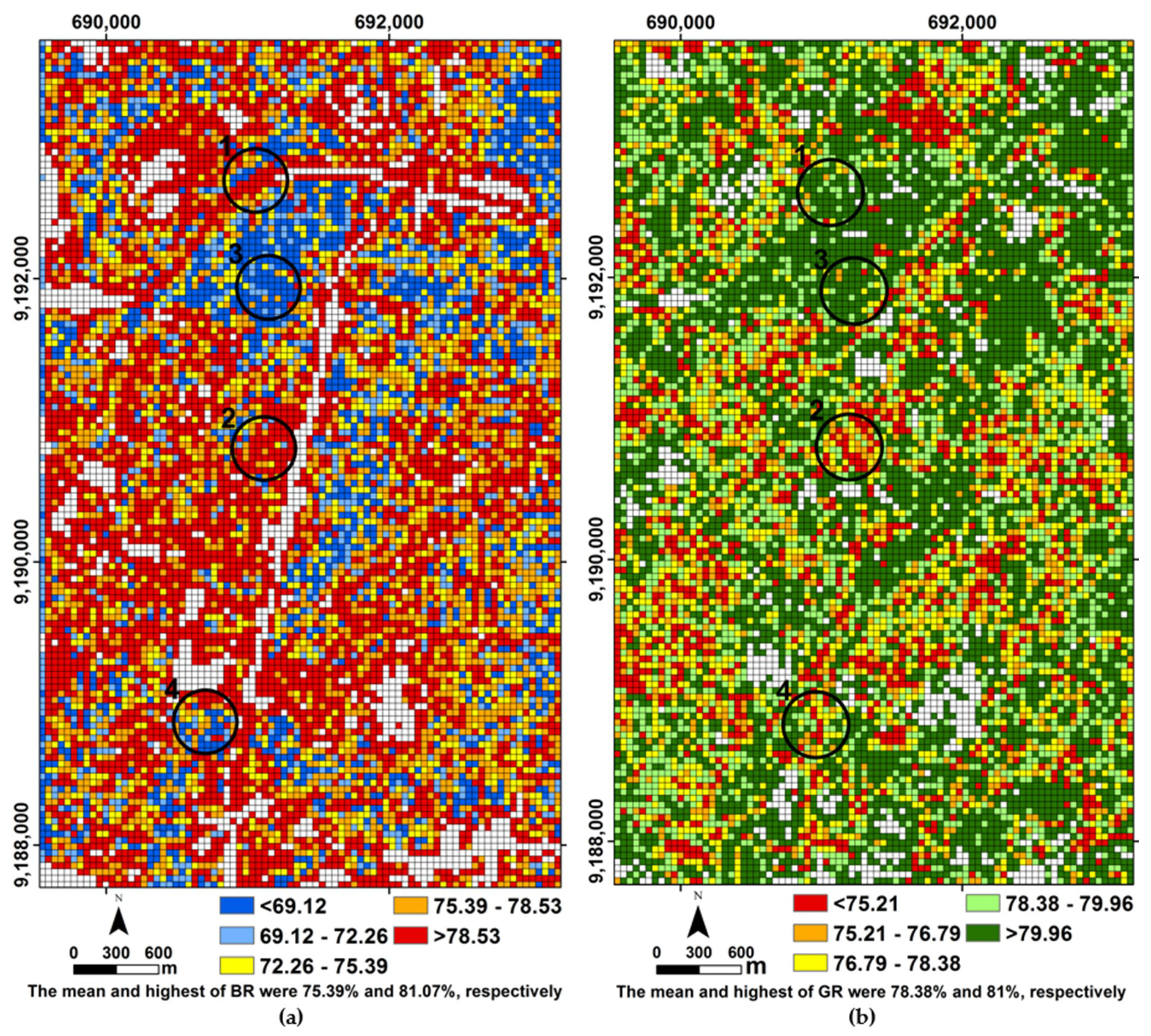
3.2.2. Validation of SFH
3.2.3. Built-Up Volume (BV)
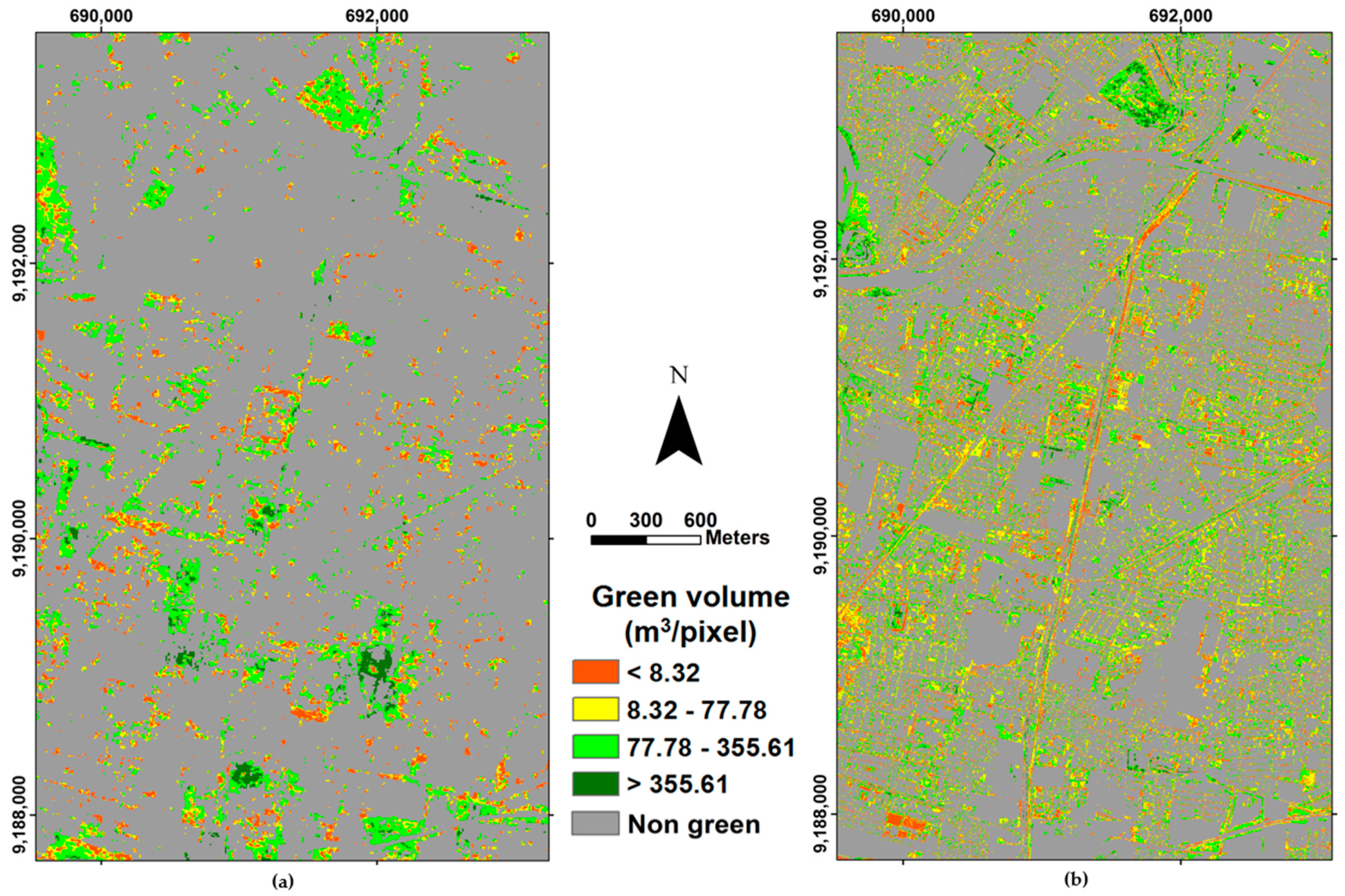
3.2.4. Green Volume (GV)
3.3. Urban Expansion
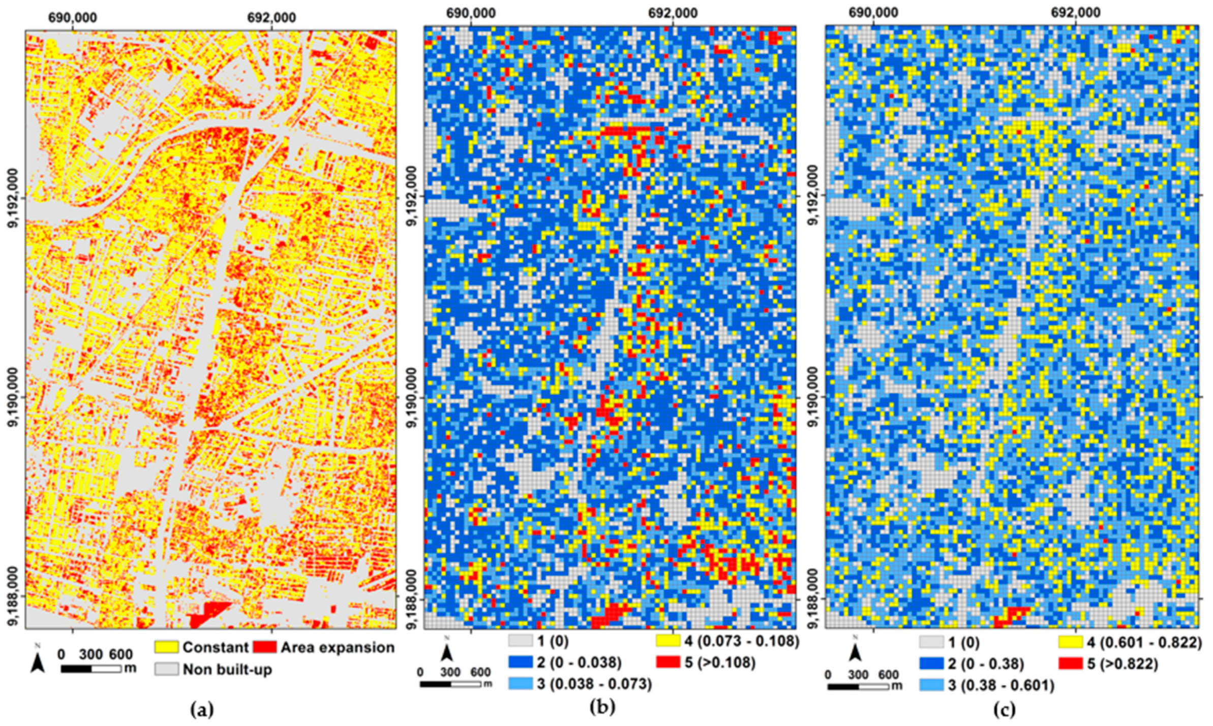
3.3.1. Patch Metric of the Built-Up and Green Area Expansions
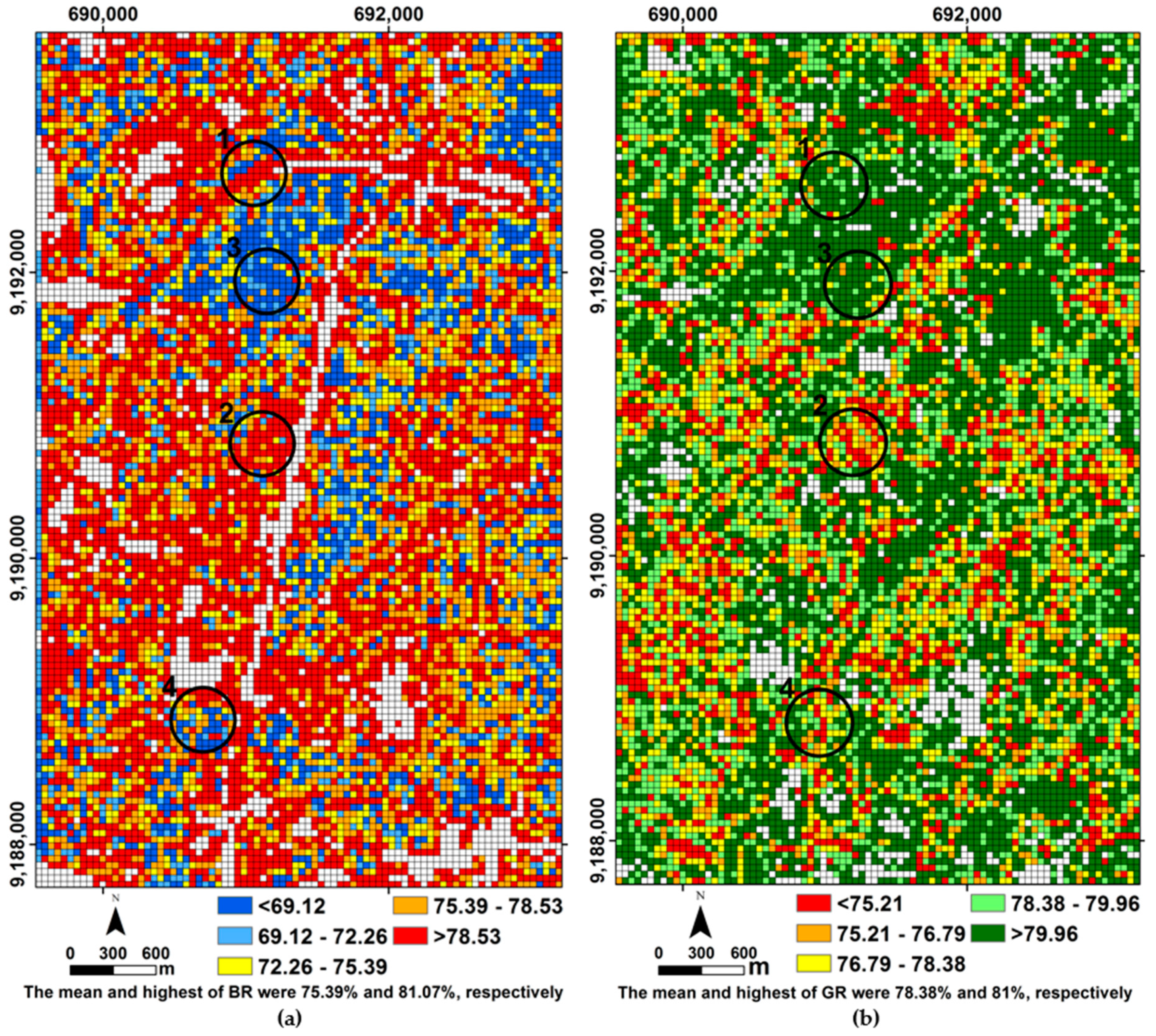
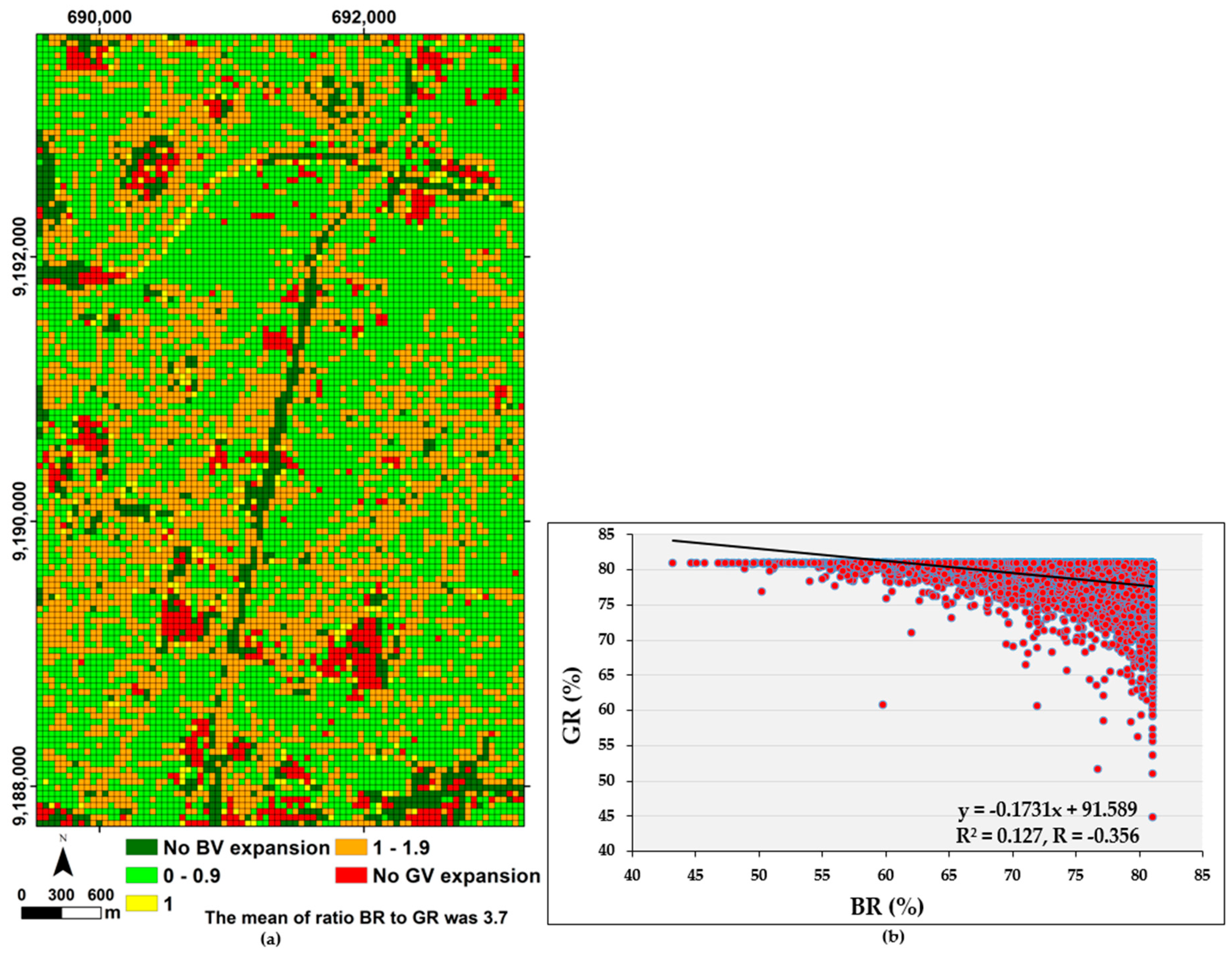
3.3.2. Built-Up and Green Volume Expansion Rate
4. Discussion
5. Conclusions
Author Contributions
Funding
Acknowledgments
Conflicts of Interest
References
- United Nations Department of Economic and Social Affairs Population Division (DESA, UN). World Population Prospects: The 2015 Revision, Key Findings and Advance Tables; United Nations: New York, NY, USA, 2015; Volume 1. [Google Scholar]
- Chen, L.; Yang, X.; Chen, L.; Li, L. Impact assessment of land use planning driving forces on environment. Environ. Impact Assess. Rev. 2015, 55, 126–135. [Google Scholar] [CrossRef]
- Cohen, B. Urbanization in developing countries: Current trends, future projections, and key challenges for sustainability. Technol. Soc. 2006, 28, 63–80. [Google Scholar] [CrossRef]
- Nor, A.N.M.; Corstanje, R.; Harris, J.A.; Brewer, T. Impact of rapid urban expansion on green space structure. Ecol. Indic. 2017, 81, 274–284. [Google Scholar] [CrossRef]
- Tian, Y.; Jim, C.Y.; Tao, Y.; Shi, T. Landscape ecological assessment of green space fragmentation in Hong Kong. Urban For. Urban Green. 2011, 10, 79–86. [Google Scholar] [CrossRef]
- Turrini, T.; Knop, E. A landscape ecology approach identifies important drivers of urban biodiversity. Glob. Chang. Biol. 2015, 21, 1652–1667. [Google Scholar] [CrossRef] [PubMed]
- Koomen, E.; Rietveld, P.; Bacao, F. The third dimension in urban geography: The urban-volume approach. Environ. Plan. B Urban Anal. City Sci. 2009, 36, 1008–1025. [Google Scholar] [CrossRef]
- Ranagalage, M.; Estoque, R.C.; Handayani, H.H.; Zhang, X.; Morimoto, T.; Tadono, T.; Murayama, Y. Relation between urban volume and land surface temperature: A Comparative study of planned and traditional cities in Japan. Sustainability 2018, 10, 2366. [Google Scholar] [CrossRef]
- Batty, M.; Besussi, E.; Maat, K.; Harts, J. Cities: Density and diversity in space and time. Built Environ. 2003, 30, 324–337. [Google Scholar] [CrossRef]
- Handayani, H.H.; Estoque, R.C.; Murayama, Y. Estimation of built-up and green volume using geospatial techniques: A case study of Surabaya, Indonesia. Sustain. Cities Soc. 2018, 37, 581–593. [Google Scholar] [CrossRef]
- Aubrecht, C.; Steinnocher, K.; Hollaus, M.; Wagner, W. Integrating earth observation and GIScience for high resolution spatial and functional modeling of urban land use. Comput. Environ. Urban Syst. 2009, 33, 15–25. [Google Scholar] [CrossRef]
- Liu, F.; Zhang, Z.; Wang, X. Forms of urban expansion of Chinese municipalities and provincial capitals, 1970s-2013. Remote Sens. 2016, 8, 930. [Google Scholar] [CrossRef]
- Shao, Z.; Fu, H.; Fu, P.; Yin, L. Mapping urban impervious surface by fusing optical and SAR data at the decision level. Remote Sens. 2016, 8, 945. [Google Scholar] [CrossRef]
- Lindquist, E.J.; D’Annunzio, R. Assessing global forest land-use change by object-based image analysis. Remote Sens. 2016, 8, 678. [Google Scholar] [CrossRef]
- Thapa, R.B.; Murayama, Y. Examining spatiotemporal urbanization patterns in Kathmandu Valley, Nepal: Remote sensing and spatial metrics approaches. Remote Sens. 2009, 1, 534–556. [Google Scholar] [CrossRef]
- McDonnell, M.J.; Hahs, A.K. The use of gradient analysis studies in advancing our understanding of the ecology of urbanizing landscapes: Current status and future directions. Landsc. Ecol. 2008, 23, 1143–1155. [Google Scholar] [CrossRef]
- Hung, W.C.; Chen, Y.C.; Cheng, K.S. Comparing landcover patterns in Tokyo, Kyoto, and Taipei using ALOS multispectral images. Landsc. Urban Plan. 2010, 97, 132–145. [Google Scholar] [CrossRef] [Green Version]
- Plexida, S.G.; Sfougaris, A.I.; Ispikoudis, I.P.; Papanastasis, V.P. Selecting landscape metrics as indicators of spatial heterogeneity-Acomparison among Greek landscapes. Int. J. Appl. Earth Obs. Geoinf. 2014, 26, 26–35. [Google Scholar] [CrossRef]
- Foody, M.G. Status of land cover classification accuracy assessment. Remote Sens. Environ. 2002, 80, 185–201. [Google Scholar] [CrossRef]
- Olofsson, P.; Foody, G.M.; Herold, M.; Stehman, S.V.; Woodcock, C.E.; Wulder, M.A. Good practices for estimating area and assessing accuracy of land change. Remote Sens. Environ. 2014, 148, 42–57. [Google Scholar] [CrossRef] [Green Version]
- Leichtle, T.; Geiß, C.; Wurm, M.; Lakes, T.; Taubenböck, H. Unsupervised change detection in VHR remote sensing imagery—An object-based clustering approach in a dynamic urban environment. Int. J. Appl. Earth Obs. Geoinf. 2017, 54, 15–27. [Google Scholar] [CrossRef]
- Zhang, P. Spatiotemporal features of the three-dimensional architectural landscape in Qingdao, China. PLoS ONE 2015, 10, e0137853. [Google Scholar] [CrossRef] [PubMed]
- Wurm, M.; Taubenböck, H.; Esch, T.; Fina, S.; Siedentop, S. The changing face of urban growth: An analysis using earth observation data. In Proceedings of the Joint Urban Remote Sensing Event 2013, Sao Paulo, Brazil, 21–23 April 2013; Volume 856, pp. 4–7. [Google Scholar]
- Chen, Z.; Gao, B.; Devereux, B. State-of-the-art: DTM generation using airborne LiDAR data. Sensors 2017, 17, 150. [Google Scholar] [CrossRef] [PubMed]
- Walikota Surabaya. The Regulation of Surabaya City Number 12 Year 2014 Concerning Spatial Plan of Surabaya for 2014–2034; Walikota Surabaya: Surabaya, Indonesia, 2014. [Google Scholar]
- Badan Pusat Statistik Kota Surabaya. Surabaya Dalam Angka 2017; Badan Pusat Statistik Kota Surabaya: Surabaya, Indonesia, 2017.
- Badan Pusat Statistik (BPS) Kota Surabaya. Statistik Daerah Kota Surabaya 2017; Badan Pusat Statistik (BPS) Kota Surabaya: Surabaya, Indonesia, 2017.
- Takaku, J.; Tadono, T. PRISM on-orbit geometric calibration and DSM performance. IEEE Trans. Geosci. Remote Sens. 2009, 47, 4060–4073. [Google Scholar] [CrossRef]
- Takaku, J.; Tadono, T.; Tsutsui, K. Generation of high resolution global DSM from ALOS PRISM. In Proceedings of the International Archives of the Photogrammetry, Remote Sensing and Spatial Information Sciences—ISPRS Archives, Suzhou, China, 14–16 May 2014; Volume 40, pp. 243–248. [Google Scholar]
- Chen, L.C.; Teo, T.A.; Kuo, C.Y.; Rau, J.Y. Shaping polyhedral buildings by the fusion of vector maps and lidar point clouds. Photogramm. Eng. Remote Sens. 2008, 74, 1147–1157. [Google Scholar] [CrossRef]
- Lohani, B.; Singh, R. Effect of data density, scan angle, and flying height on the accuracy of building extraction using LiDAR data. Geocarto Int. 2008, 23, 81–94. [Google Scholar] [CrossRef] [Green Version]
- Heidemann, K.H. Lidar Base Specification; (Ver. 1.3, February 2018): U.S. Geological Survey Techniques and Methods, Book 11, Chap. B4; U.S. Geological Survey: Sioux Falls, SD, USA, 2018.
- Dinas Cipta Karya dan Tata Ruang (DCKTR) Kota Surabaya. LiDAR and Aerial Mapping of Surabaya; Dinas Cipta Karya dan Tata Ruang (DCKTR) Kota Surabaya: Surabaya, Indonesia, 2016. [Google Scholar]
- Abidin, H.Z. Strengthening geospatial information management in Indonesia geospatial information for national sustainable development. In Proceedings of the 5th High Level Forum United Nations: Global Geospatial Information Management, Mexico City, Mexico, 28–30 November 2017. [Google Scholar]
- Matindas, R.W.; Puntodewo; Purnawan, B. Development of National Spatial Data Infrastructure in Indonesia. In NSDI’s Development, FIG Working Week; International Federation of Surveyors (FIG): Athens, Greece, 2004; pp. 1–6. [Google Scholar]
- Environmental Systems Research Institute (ESRI). Indonesia NSDI: One Map for the Nation. Available online: https://bit.ly/2E5eyM9 (accessed on 13 September 2018).
- Japan Aerospace Exploration Agency (JAXA). ALOS Product Format Description; Japan Aerospace Exploration Agency (JAXA): Tsukuba, Japan, 2010. [Google Scholar]
- Shimada, M.; Tadono, T.; Rosenqvist, A. Advanced land observing satellite (ALOS) and monitoring global environmental change. Proc. IEEE 2010, 98, 780–799. [Google Scholar] [CrossRef]
- Dinas Cipta Karya dan Tata Ruang (DCKTR) Kota Surabaya. A Utility Map; Dinas Cipta Karya dan Tata Ruang (DCKTR) Kota Surabaya: Surabaya, Indonesia, 2002. [Google Scholar]
- Badan Perencanaan dan Pembangunan Kota (Bappeko) Surabaya. A Land Use Map of Surabaya; Badan Perencanaan dan Pembangunan Kota Surabaya: Surabaya, Indonesia, 2008. [Google Scholar]
- Tadono, T.; Shimada, M.; Murakami, H.; Mukaida, A.; Takaku, J.; Kawamoto, S. Preliminary results of calibration for ALOS optical sensors and validation of generated PRISM DSM. Proc. SPIE 2006, 6361, U25–U32. [Google Scholar]
- Gianinetto, M.; Scaioni, M. Automated geometric correction of high-resolution pushbroom satellite data. Photogramm. Eng. Remote Sens. 2008, 74, 107–116. [Google Scholar] [CrossRef]
- Deng, H.; Huang, S.; Wang, Q.; Pan, Z.; Xin, Y. Geometric accuracy assessment and correction of imagery from Chinese Earth Observation satellites (HJ-1 A/B, cbers-02C and ZY-3). ISPRS Arch. Proc. Int. Arch. Photogramm. Remote Sens. Spat. Inf. Sci. 2014, 40, 71–78. [Google Scholar] [CrossRef]
- Geospatial Information Agency Indonesia Indonesian Geospatial Reference System 2013 (SRGI2013). Available online: http://srgi.big.go.id/srgi/ (accessed on 10 July 2018).
- Simpson, J.J.; Mclntire, T.J.; Sienko, M. An improved hybrid clustering algorithm for natural scenes. IEEE Trans. Geosci. Remote Sens. 2000, 38, 1016–1032. [Google Scholar] [CrossRef]
- Liu, W.; Gopal, S.; Woodcock, C.E. Uncertainty and confidence in land cover classification using a hybrid classifier approach. Photogramm. Eng. Remote Sens. 2004, 70, 963–971. [Google Scholar] [CrossRef]
- Lu, D.; Weng, Q. A survey of image classification methods and techniques for improving classification performance. Int. J. Remote Sens. 2007, 28, 823–870. [Google Scholar] [CrossRef] [Green Version]
- Phiri, D.; Morgenroth, J. Developments in Landsat land cover classification methods: A review. Remote Sens. 2017, 9, 967. [Google Scholar] [CrossRef]
- Thapa, R.B.; Murayama, Y. Urban mapping, accuracy, & image classification: A comparison of multiple approaches in Tsukuba City, Japan. Appl. Geogr. 2009, 29, 135–144. [Google Scholar] [CrossRef] [Green Version]
- Lillesand, T.M.; Kieffer, R.W.; Chipman, J.W. Remote Sensing and Image Interpretation, 5th ed.; John Wiley: New York, NY, USA, 2004; ISBN 0471451525. [Google Scholar]
- Kim, M.; Madden, M.; Warner, T.A. Forest type mapping using object-specific texture measures from multispectral Ikonos imagery: Segmentation quality and image classification issues. Photogramm. Eng. Remote Sens. 2009, 75, 819–829. [Google Scholar] [CrossRef]
- Liu, D.; Xia, F. Assessing object-based classification: Advantages and limitations. Remote Sens. Lett. 2010, 1, 187–194. [Google Scholar] [CrossRef]
- Bangira, T.; Alfieri, S.M.; Menenti, M.; van Niekerk, A.; Vekerdy, Z. A spectral unmixing method with ensemble estimation of endmembers: Application to flood mapping in the Caprivi floodplain. Remote Sens. 2017, 9, 1013. [Google Scholar] [CrossRef]
- Yang, X.; Zhao, S.; Qin, X.; Zhao, N.; Liang, L. Mapping of urban surface water bodies from sentinel-2 MSI imagery at 10 m resolution via NDWI-based image sharpening. Remote Sens. 2017, 9, 596. [Google Scholar] [CrossRef]
- Baghzouz, M.; Devitt, D.A.; Fenstermaker, L.F.; Young, M.H. Monitoring vegetation phenological cycles in two different semi-arid environmental settings using a ground-based NDVI system: A potential approach to improve satellite data interpretation. Remote Sens. 2010, 2, 990–1013. [Google Scholar] [CrossRef]
- Johnson, B.; Bragais, M.; Endo, I.; Magcale-Macandog, D.; Macandog, P. Image segmentation parameter optimization considering within- and between-segment heterogeneity at multiple scalelevels: Test case for mapping residential areas using Landsat Imagery. ISPRS Int. J. Geo Inf. 2015, 4, 2292–2305. [Google Scholar] [CrossRef]
- Coburn, C.A.; Roberts, A.C.B. A multiscale texture analysis procedure for improved forest stand classification. Int. J. Remote Sens. 2004, 25, 4287–4308. [Google Scholar] [CrossRef] [Green Version]
- Feng, Q.; Liu, J.; Gong, J. UAV Remote sensing for urban vegetation mapping using random forest and texture analysis. Remote Sens. 2015, 7, 1074–1094. [Google Scholar] [CrossRef]
- Yang, M.D.; Huang, K.S.; Kuo, Y.H.; Tsai, H.P.; Lin, L.M. Spatial and spectral hybrid image classification for rice lodging assessment through UAV imagery. Remote Sens. 2017, 9, 583. [Google Scholar] [CrossRef]
- Benz, U.C.; Hofmann, P.; Willhauck, G.; Lingenfelder, I.; Heynen, M. Multi-resolution, object-oriented fuzzy analysis of remote sensing data for GIS-ready information. ISPRS J. Photogramm. Remote Sens. 2004, 58, 239–258. [Google Scholar] [CrossRef] [Green Version]
- Laliberte, A.S.; Rango, A.; Havstad, K.M.; Paris, J.F.; Beck, R.F.; McNeely, R.; Gonzalez, A.L. Object-oriented image analysis for mapping shrub encroachment from 1937 to 2003 in southern New Mexico. Remote Sens. Environ. 2004, 93, 198–210. [Google Scholar] [CrossRef]
- Sithole, G.; Vosselman, G. Experimental comparison of filter algorithms for bare-Earth extraction from airborne laser scanning point clouds. ISPRS J. Photogramm. Remote Sens. 2004, 59, 85–101. [Google Scholar] [CrossRef]
- Zhang, K.; Whitman, D. Comparison of three algorithms for filtering airborne LiDAR data. Photogramm. Eng. Remote Sens. 2005, 71, 313–324. [Google Scholar] [CrossRef]
- Wang, C.K.; Tseng, Y.H. DEM generation from airborne LiDAR data by an adaptive dual-directional slope filter. In Proceedings of the International Archives of Photogrammetry Remote Sensing and Spatial Information Sciences, Vienna, Austria, 5–7 July 2010; pp. 628–632. [Google Scholar]
- Bagan, H.; Yamagata, Y. Land-cover change analysis in 50 global cities by using a combination of Landsat data and analysis of grid cells. Environ. Res. Lett. 2014, 9, 2000–2010. [Google Scholar] [CrossRef]
- McGarigal, K.; Cushman, S.A.; Ene, E. FRAGSTATS v4: Spatial Pattern Analysis Program for Categorical and Continuous Maps; the University of Massachusetts Amherst: Amherst, MA, USA, 2012. [Google Scholar]
- LaGro, J. Assessing patch shape in landscape mosaics. Photogramm. Eng. Remote Sens. 1991, 57, 285–293. [Google Scholar]
- Zhang, Y.; Van den Berg, A.E.; Van Dijk, T.; Weitkamp, G. Quality over quantity: Contribution of urban green space to neighborhood satisfaction. Int. J. Environ. Res. Public Health 2017, 14, 535. [Google Scholar] [CrossRef] [PubMed]
- Latinopoulos, D.; Mallios, Z.; Latinopoulos, P. Valuing the benefits of an urban park project: A contingent valuation study in Thessaloniki, Greece. Land Use Policy 2016, 55, 130–141. [Google Scholar] [CrossRef]
- Park, S. A preliminary study on connectivity and perceived values of community green spaces. Sustainability 2017, 9, 692. [Google Scholar] [CrossRef]
- Parsons, R. Conflict between ecological sustainability and environmental aesthetics: Conundrum, canärd or curiosity. Landsc. Urban Plan. 1995, 32, 227–244. [Google Scholar] [CrossRef]
- van den Berg, A.E.; van Winsum-Westra, M. Manicured, romantic, or wild? The relation between need for structure and preferences for garden styles. Urban For. Urban Green. 2010, 9, 179–186. [Google Scholar] [CrossRef]
- Wentz, E.A.; York, A.M.; Alberti, M.; Conrow, L.; Fischer, H.; Inostroza, L.; Jantz, C.; Pickett, S.T.A.; Seto, K.C.; Taubenböck, H. Six fundamental aspects for conceptualizing multidimensional urban form: A spatial mapping perspective. Landsc. Urban Plan. 2018, 179, 55–62. [Google Scholar] [CrossRef]
- Tomás, L.; Fonseca, L.; Almeida, C.; Leonardi, F. Urban population estimation based on residential buildings volume using IKONOS-2 images and lidar data. Int. J. Remote Sens. 2015. [Google Scholar] [CrossRef]
- The President of The Republic of Indonesia. Law of Republic Indonesia Number 26 Year 2007 Corncerning Spatial Planning; Jakarta, Indonesia, 2007.


| Data | Date | Source | Description | Purpose |
|---|---|---|---|---|
| ALOS image | 17 July 2010 | [37] |
|
|
| ALOS DSM | ||||
| LiDAR DSM | Acquired on May–August 2016 | [33] |
|
|
| LiDAR-derived DTM | ||||
| Orthophoto | ||||
| Base map | 2002 | [39] |
|
|
| Building map | ||||
| Land use map | 2008 | [40] | Scale of 1:10,000 | The previous land use map was used to conduct the accuracy assessment of LU/LC map 2010 and 2016. |
| Name (Unit) | Abbreviation (Range) | Description | Equation | |
|---|---|---|---|---|
| Area of built-up (hectares) | AREA (AREA > 0, without limit) | To examine the area expansion in term of size. | aij = area (m2) of patch ij. | (4) |
| Contiguity index (none) | CONTIG (0 ≤ CONTIG ≤ 1) | To examine the pattern of area expansion regarding the spatial contiguity of patches. | cijr = contiguity value for pixel r in patch ij. v = sum of the values in a 3-by-3 cell template (13 in this case). aij = area of patch ij in terms of number of cells. | (5) |
| Type of LU/LC | Area (km2) | Change (%) | |
|---|---|---|---|
| 2010 | 2016 | ||
| Built-up | 9.49 | 10.58 | 11.54 |
| Road pavement | 4.82 | 3.80 | −21.30 |
| Green space | 3.09 | 6.06 | 95.61 |
| Waterbody | 0.47 | 0.69 | 46.93 |
| Bareland | 4.64 | 1.39 | −70.00 |
| Classes | LU/LC in 2010 | LU/LC in 2016 | ||
|---|---|---|---|---|
| PA (%) | UA (%) | PA (%) | UA (%) | |
| Built-up | 85.84 | 89.82 | 87.61 | 95.52 |
| Green space | 81.9 | 80.00 | 82.86 | 84.00 |
| Road pavement | 83.00 | 83.80 | 87.00 | 86.10 |
| Bareland | 81.32 | 77.10 | 84.78 | 80.40 |
| Waterbody | 83.52 | 84.40 | 90.11 | 88.2 |
| OA (%) | 83.20 | 86.43 | ||
| Κ | 0.79 | 0.83 | ||
| Kernel Size (pixel) | Grid Size (m) | DTM (m) | RMSe of Interpolation (m) | The Highest Values SFH (m) | |
|---|---|---|---|---|---|
| Lowest | Highest | ||||
| 3 | 15 | −31.23 | 76.17 | 4.79 | 87.41 |
| 5 | 25 | −30.65 | 61.77 | 4.87 | 89.43 |
| 7 | 35 | −30.53 | 58.12 | 4.99 | 89.78 |
| 9 | 45 | −30.47 | 54.27 | 5.04 | 89.01 |
| 11 | 55 | −30.48 | 46.55 | 5.29 | 89.38 |
| 15 | 75 | −31 | 39.23 | 5.6 | 91.03 |
| 21 | 105 | −31.04 | 36.97 | 6.09 | 93.07 |
| 27 | 135 | −31.03 | 30.24 | 6.42 | 93.79 |
| 33 | 165 | −31.03 | 28.27 | 6.63 | 95.54 |
| 39 | 195 | −31.05 | 25.68 | 7.29 | 95.85 |
| 45 | 225 | −31.03 | 25.69 | 7.75 | 97.75 |
| Built-Up Volume (m3/pixel) | Height (m) | Number of Storey | Portion | ||
|---|---|---|---|---|---|
| 2010 | 2016 | Change (%) | |||
| <162.4 | <7 | 1–2 | 82.07% | 65.66% | −16.41 |
| 162.4–368.64 | 7–14 | 3–4 | 14.71% | 30.67% | 15.96 |
| 368.64–575 | 14–23 | 5–7 | 1.91% | 2.13% | 0.22 |
| 575–781.13 | 24–31 | 8–9 | 0.57% | 0.51% | −0.06 |
| >781.13 | >31 | >9 | 0.74% | 1.03% | 0.29 |
| Green Volume (m3/pixel) | Height (m) | Portion | ||
|---|---|---|---|---|
| 2010 | 2016 | Change (%) | ||
| <8.32 | <0.3 | 3.73% | 12.73% | 8.99 |
| 8.32–77.78 | 0.3–3 | 30.68% | 35.48% | 4.80 |
| 77.78–355.61 | 3–14 | 58.48% | 49.00% | −9.48 |
| >355.61 | >14 | 7.10% | 2.79% | −4.31 |
| CONTIG BA | CONTIG BA | AREA GA | CONTIG GA | |
|---|---|---|---|---|
| AREA BA | 1 | 0.762 | −0.111 | −0.12 |
| CONTIG BA | 1 | −0.21 | −0.05 | |
| AREA GA | 1 | 0.735 | ||
| CONTIG GA | 1 |
© 2018 by the authors. Licensee MDPI, Basel, Switzerland. This article is an open access article distributed under the terms and conditions of the Creative Commons Attribution (CC BY) license (http://creativecommons.org/licenses/by/4.0/).
Share and Cite
Handayani, H.H.; Murayama, Y.; Ranagalage, M.; Liu, F.; Dissanayake, D. Geospatial Analysis of Horizontal and Vertical Urban Expansion Using Multi-Spatial Resolution Data: A Case Study of Surabaya, Indonesia. Remote Sens. 2018, 10, 1599. https://doi.org/10.3390/rs10101599
Handayani HH, Murayama Y, Ranagalage M, Liu F, Dissanayake D. Geospatial Analysis of Horizontal and Vertical Urban Expansion Using Multi-Spatial Resolution Data: A Case Study of Surabaya, Indonesia. Remote Sensing. 2018; 10(10):1599. https://doi.org/10.3390/rs10101599
Chicago/Turabian StyleHandayani, Hepi H., Yuji Murayama, Manjula Ranagalage, Fei Liu, and DMSLB Dissanayake. 2018. "Geospatial Analysis of Horizontal and Vertical Urban Expansion Using Multi-Spatial Resolution Data: A Case Study of Surabaya, Indonesia" Remote Sensing 10, no. 10: 1599. https://doi.org/10.3390/rs10101599