Abstract
Despite the recognized effectiveness of LiDAR in penetrating forest canopies, its capability for archaeological prospection can be strongly limited in areas covered by dense vegetation for the detection of subtle remains scattered over morphologically complex areas. In these cases, an important contribution to improve the identification of topographic variations of archaeological interest is provided by LiDAR-derived models (LDMs) based on relief visualization techniques. In this paper, diverse LDMs were applied to the medieval site of Torre Cisterna to the north of Melfi (Southern Italy), selected for this study because it is located on a hilly area with complex topography and thick vegetation cover. These conditions are common in several places of the Apennines in Southern Italy and prevented investigations during the 20th century. Diverse LDMs were used to obtain maximum information and to compare the performance of both subjective (through visual inspections) and objective (through their automatic classification) methods. To improve the discrimination/extraction capability of archaeological micro-relief, noise filtering was applied to Digital Terrain Model (DTM) before obtaining the LDMs. The automatic procedure allowed us to extract the most significant and typical features of a fortified settlement, such as the city walls and a tower castle. Other small, subtle features attributable to possible buried buildings of a habitation area have been identified by visual inspection of LDMs. Field surveys and in-situ inspections were carried out to verify the archaeological points of interest, microtopographical features, and landforms observed from the DTM-derived models, most of them automatically extracted. As a whole, the investigations allowed (i) the rediscovery of a fortified settlement from the 11th century and (ii) the detection of an unknown urban area abandoned in the Middle Ages.
1. Introduction
The identification, analysis, and survey of archaeological remains and proxy indicators is a complex challenge especially in areas covered by dense vegetation, as wooded and forest land. The constraints are due to (i) vegetation cover type, density, and height, as well as (ii) dimensions and state of conservation of archaeological remains.
The difficulties in the documentation, survey, and material collection increase in areas characterized by dense understory vegetation. In this condition, the presence of scattered building materials further increases the difficulty in the identification of archaeological proxy indicators linked to micro-topographical and landform variations. To face these challenges, remote sensing based on LiDAR (Light Detection and Ranging) can be fruitfully applied to achieve unique performance in detecting and surveying archaeological features and remains, even in rain forest and densely vegetated areas with close canopy [1]. For example, Chase et al. [2] portrayed the Maya landscape topography and also detected structures, causeways, and agricultural terraces in the rainforest of Caracol (Belize). Evans et al. [3], using LiDAR, identified and reconstructed the urban landscape in Angkor (Cambodia) improving knowledge on Khmer civilization and providing new elements related to the reasons of its decline, caused by both unsustainable modes of subsistence and climate variations. Doneus et al. [4] tested the penetration capability of LiDAR for archaeological purposes in forested areas, detecting topographic earthwork features of a hillfort, ramparts, and round barrows, dated to Iron Age and hidden in a forest area in eastern Austria. In Northwest Spain, integrated geomatic applications based on LiDAR data and UAV-assisted photogrammetry enabled detection of ancient Roman gold mining sites [5] and water supply systems and pine forests [6]. In Italy, the integrated use of LiDAR, UAV, aerial thermography, and multispectral satellite imagery, in the Etruscan site of San Giovenale at about 60 km NW of Rome, revealed a large variety of archaeological features, including a necropolis and a road, tumulus under canopy, most of them under canopy [7].
Despite the recognized effectiveness of LiDAR in penetrating forest canopies, its capability for archaeological prospection could be strongly limited by vegetation cover, as demonstrated by Hutson [8] who evaluated the correlations between vegetation height, ground return density, and the ability to identify archeological features, with particular reference to micro-relief due to shallow remains and small structures [9]. In these cases, the LiDAR-based analysis requires special attention both to point clouds processing and classification to avoid that the removal of low vegetation can also determine loss of archaeological information. Furthermore, an important contribution to improve the identification of archaeological features is provided by LiDAR-Derived Models (LDMs) based on relief visualization techniques. Since the pioneering LiDAR applications in archaeology [10], relief visualization techniques, such as the popular hill shading, vertical exaggeration, and topographical modeling (slope, convexity) have been widely used. However, they exhibit some limits which have been recently overcome by Local Relief Model [11], Sky-view factor [12], and Openness [13].
The added value of LDMs is particularly noticeable for small structures and micro-relief, particularly in hilly settlements under dense vegetated areas, for example, deserted medieval villages. The desertion of villages was a global phenomenon which interested most of Europe from the 12th to 15th century due to a number of social, economic, political, and military factors which, coupled with epidemic and pandemic events, caused demographic decreases and the displacement of people from villages and hamlets to towns [14,15]. This strongly changed the characteristics and features of settlement patterns, causing a series of continuous expansions, contractions, and reorganizations of urban and rural landscape. For these reasons, in Europe, deserted medieval settlements represent a great amount of archaeological heritage, that deserve to be studied and protected, much more than what has been done until today. During the second half of the 20th century, more attention has been paid to medieval agrarian landscapes and deserted villages [11]. Nevertheless, the identification of abandoned settlements is still a critical issue because they are hidden by dense vegetation cover, generally located in hilly zones, and, in many cases, characterized by complex topographic features. Finally, they are usually affected by erosion processes which prevent the soil deposition (typically of ancient structures in flat settlements) and cause degradation (if not the loss) of building materials frequently scattered all over, thus making their detection difficult. In these cases, LDMs are the best tools for archaeological prospecting even if up to now, due to the complexity briefly discussed above, only a few studies have been conducted on abandoned medieval villages using LiDAR. Corns and Shaw [16] investigated the abandoned castle and settlement in Newtown Jerpoint in Ireland, Heine [17] conducted studies in the medieval remains of Nienover in the Lower Saxony, Lasaponara and Masini performed surveys and investigations in two deserted medieval villages in Basilicata (South Italy) [18,19], and finally, Krivanek R. [20] identified remains of abandoned villages and small castles in Bohemia located in inaccessible forested areas. Landscape scale investigations have been also conducted by Simmons [21] in the medieval rural landscapes between the East Fen and the Tofts in south-east Lincolnshire, and by Baubiniene et al. in Lithuania [22].
For the purpose of our analyses, several LDMs were applied to obtain the maximum of information and to compare their performance both subjectively, through visual inspections, and objectively through their automatic classification.
The investigations were carried out in the medieval site of Torre Cisterna in Basilicata (Southern Italy), selected because it is an emblematic case study of settlement abandoned in Middle Ages. It is located on a hilly plateau and covered by vegetation so thick to prevent investigations for all the 20th century. The reason for experimenting this approach in Torre di Cisterna is the high number of deserted sites in Medieval times (especially in the late Middle Age), all over the Europe (only in the small Basilicata region about 70 abandoned villages have been recorded [23]). In most cases, they are located on hilly reliefs, generally covered by dense vegetation in wooded area, and characterized by the presence of a castle, walls, and an inhabited area. It is expected that over the centuries, the remains of the castle and city walls should be more preserved compared to buildings of the habitation area made up of smaller structures sometimes in wood.
2. Materials and Methods
2.1. Study Area
Torre di Cisterna (in English, “Tower of Cisterna”) is a hilly plateau with the maximum height of 668 m located in the Northeast of the Basilicata Region (South of Italy) in the municipality of Melfi, between 41°02′42″ and 41°03′29″ latitudes north and 15°35′06″ and 15°35′56″ east longitudes, at the boundary with the Campania and Apulia regions (see Figure 1a,b).
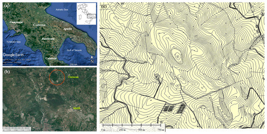
Figure 1.
(a) Location of Torre di Cisterna at North of Basilicata (Southern Italy); (b) Orthophoto including the investigated area located at Northwest of Melfi; (c) Map of the territory of Cisterna: the red circle denotes the hilly plateau where the medieval settlement that is the object of investigation is located.
From the geological point of view, Torre di Cisterna is located in the easternmost portion of the southern Apennine, a thrust and fold belt chain. The site is close to the front of the Apennine napes where the typical Oligo-Miocene sediments outcrop. These sediments gradually replace the volcanic deposits of the Pleistocene Vulture volcano whose products mark out the territory at south of the area herein investigated.
The Torre di Cisterna hill (Figure 1c), that is part of the Ofanto river basin, is made up of Miocene deposits such as microgranular whitish or yellowish limestones, light-colored calcarenites, marl and clay schists, whitish or yellowish sandstones, and pudding stones (Formazione della Daunia, in English: Daunia Formation [24]). The area surrounding the hill is made up of marls, calcareous marl, silty clays (western, northern and southern areas), and polygenic conglomerate (eastern).
The hill is covered by coppice forest composed mainly of three species of oaks; the common oak (Quercus robur), pubescent oak (Quercus pubescens), and Turkey oak (Quercus cerris), with a undergrowth made from blackberry bushes (Rubus ulmifolius), ferns (Polystichum setiferum), wild blackthorn (Prunus spinosa), ferula (Ferula communis), hawthorn (Crataegus monogyna), butcher’s broom (Ruscus aculeatus), and rose hip. The forest borders with land cultivated with cereals.
The whole area was characterized by a continuous human frequentation particularly important during (i) the Roman imperial period, as evident by the presence of Roman farms, necropolis, and ruins of a villa (Figure 1), and (ii) the Middle Ages.
In this paper, we focused our investigations on the hilly plateau indicated with the red circle in Figure 1c, thought to be a settlement founded at the beginning of the XI century, along with other sites such as Civitate, Dragonara, Fiorentino, Montecorvino, Tertiveri, as a node of the Byzantine Lime [25]. The latter was a defense system, built in 1018, marking the boundaries of the Byzantine Apulia with the western territories of Southern Italy where Longobards were settled.
Cisterna is attested in 1025 when it was Episcopal seat and therefore the settlement was not a simple ‘terra’ but a ‘civitas’. In the Medieval times ‘terra’ generally indicated hamlet or a village which not always was protected by walls. The ‘civitas’ played an important institutional role and for this reason was generally protected by walls.
Unfortunately, Cisterna was destroyed by the Norman Roberto il Guiscardo in 1074 and fifteen years later it was no longer a seat of diocese
We do not know if after this event it was abandoned or suffered a gradual depopulation. In this regard, historical sources do not help to clarify this issue. It must be said that the first census of Southern Italy carried out in 1270 does not include Cisterna: the settlement was probably no longer inhabited.
Cisterna, founded under the best auspices, being from the beginning the seat a diocese, did not exist anymore. However, its history as a fortified site is longer. It is very likely that from the 13th century on, the site began to be called Torre di Cisterna as attested in a list of castles of the Kingdom of Southern Italy (known also Statutum de reparatione castrorum) to be repaired, issued by the Emperor Frederick II around 1240 [26]. This list included two different typologies of castles, castrum and domus. The former included castles with military and defense functions, the latter were rural residences, although characterized by constructive elements that lead back to typical fortified architecture. Some of them, including Torre di Cisterna (cited as domus in the Statutum de reparatione castrorum), were used by the Emperor himself when he hunted in the reserve of Melfi [27].
From the thirteenth century onwards, the documents only refer to a castle which had to consist of a tower-shaped structure as attested by the toponym (Torre) and by historic maps dated to the half of the 17th century (Figure 2a) and the first decade of the 19th century (Figure 2b,c). The images in Figure 2a–c unequivocally show a tower-shaped castle. In these three pictures, with different levels of detail, the tower stands out from a quadrangular basement to form a truncated pyramid architecture.
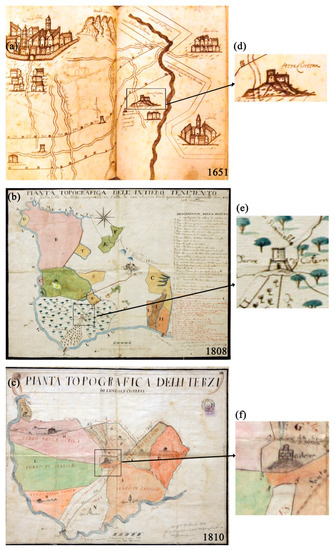
Figure 2.
Historic cartographic maps including Torre Cisterna dated to 1651–52, 1808, and 1810. In particular: (a) State Archive of Foggia, Dogana delle Pecore, Cartography of ship tracks made by Ettore Capelatro, dimensions 250 × 240 mm, 1651–1652; (b) State Archive of Potenza. Registry of Azienda Doria Pamphili. Topographic Map of the territory surrounding Melfi, including Cisterna (Original italian title of the map: “Pianta Topografica dell’Intiero Tenimento di Melfi”). Water color, dimensions 520 × 680 mm, 1808, made by the Royal surveyor Francesco Sarra. (c) State Archive of Potenza. Registry of Azienda Doria Pamphili. Topographic Map of Lionessa and Cisterna (Original italian title of the map: “Pianta Topografica delli terzi di Lionessa e Cisterna”). Water color, dimensions 417 × 519 mm, 7 October 1810, made by the Royal surveyor Francesco Sarra. (d–f) are details of (a–c), respectively, depicting the tower of Cisterna.
Cisterna is not anymore mentioned in documents after Frederick II’s death, during the fights between the various factions in the second half of the 13th century. Charles I of Anjou, who succeeded Frederick II in the government of the Kingdom of Southern Italy, authorized the repopulation of the deserted settlement [28], even if the process was quite slow as attested by the circumstance that no taxations were recorded. At the end of the 15th century, they tried to repopulate Cisterna [29] but probably with poor results. In fact, in the 16th century, the territory was defined as a “difesa”, a cultivated area not accessible to pasture. During the 17th century, the presence of thick woods secured a remarkable income [30,31].
The above-mentioned historical maps (see Figure 2a–c) only report structures of the castle, whereas no remains of the village are depicted.
At present, the whole area is covered by dense vegetation and is hardly accessible. In these conditions, only LiDAR survey can provide suitable information on the archaeological ruins still present under the wood, as suggested by remains of walls and scattered building materials and pottery.
2.2. LiDAR: Technology and Data Acquisition
LiDAR is an active remote sensing technique that uses laser pulses emitted by a scanner to measure earth surface and canopy, which are mapped into 3D point clouds. The data acquisition can be performed by conventional scanners or a full waveform (FW) scanner. The first is based on discrete echo which detects one representative trigger signal for each laser beam, the second digitizes the whole signature for each backscattered pulse [32]. Therefore, compared to the conventional scanner, FW enables a more refined classification of terrain targets, providing more accurate digital terrain models (altimetrical accuracy <0.1 m) even under dense vegetation cover.
In Cisterna, LiDAR survey was carried out using a FW scanner (RIEGL LMS-Q560) on board a helicopter performed by GEOCART S.p.A.
The LiDAR data were acquired on 10 October 2014 for an area of around 600 ha. The scanner acquired data in the direction South-North and East-West, with a divergence of the radius of 0.5 mrad, and a pulse repetition rate at 240.000 Hz. The average point density value of the dataset is about 25 points/m2. The LiDAR measurement accuracy is 2 cm and, after georeferencing, the absolute accuracy of the dataset is less than 5 cm in xy and 10 cm in z (altitude).
2.3. Data Processing: From Filtering to Classification
The first step of LiDAR data processing aimed to remove noisy points and outliers. According to their three-dimensional characteristics, they can be divided into three categories: (i) isolated points, when no other cloud points are present in their neighborhoods, (ii) air points, which are far higher from the nearby rough surface (usually caused by reflections of low altitude planes or birds), and, finally, (iii) low points, lower than their adjacent ground LiDAR points, which are caused by multiple reflections of laser pulses.
In the case of Cisterna, the removal of low points has been set assuming a height lower than 0.5 m respect to other points within a ray of 5 m.
For the identification and interpretation of microrelief and structures, the classification of terrain and off terrain targets, especially in the presence of vegetation, is crucial to avoid classifying archaeological features as off terrain targets, thus loosing precious information. In fact, the accuracy of LiDAR-based DTM decreases in areas covered by shrubs and trees as in the case of Cisterna, because the reflection generated by low vegetation canopies are often mistaken as those from bare terrains [33]. Before the classification, it is fundamental to apply adequate filtering methods which improve DTM accuracy even in the presence of dense low vegetation and complex morphology, as in the case of Cisterna.
A number of filtering methods are available in the literature. They can be categorized into four groups [30] as: block-minimum, slope-based, Surface-based, and clustering/segmentation filtering.
For the surface conditions of the study area, it is expected that surface-based filtering methods should provide the best results according to Sithole and Vosselman [34]. Examples of surface-based algorithms are: progressive Triangulation Irregular Network (TIN) densification by Axelsson [35], the hierarchic based method by Briese and Pfeifer [36], Elmqvist algorithm [37] based on the concept of membrane floating upwards from beneath the point cloud (defining the bare-earth form).
The DTM of Cisterna was obtained using the progressive TIN method by Axelsson [35], embedded in Terrasolid’s Terrascan [38]. The method is comprised of two steps (see [39]): (i) the construction of an initial TIN model (starting from the lowest points in the neighborhoods with a pre-determined size) and (ii) the iterative addition of new points that (see P in Figure 3) must satisfy the following three thresholds reported in Table 1. In particular, the iteration angle threshold (α) is the maximum angle between the point to be tested P (the closest vertex of the TIN, see P in Figure 3) and its projection onto TIN facet. The iteration distance threshold (h) is the maximum distance of the normal between the TIN facet to P. The terrain angle is the threshold for the slopes of the three new TIN facets. Finally, max edge determines how close the points must be to one another before they are attached.
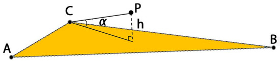
Figure 3.
Triangulated irregular network (TIN) rational model.

Table 1.
The threshold values assigned to classify ground and non-ground points.
Figure 4 shows the orthophoto (Figure 4 up) and the DTM (Figure 4 bottom) of the investigated area and its surrounding.
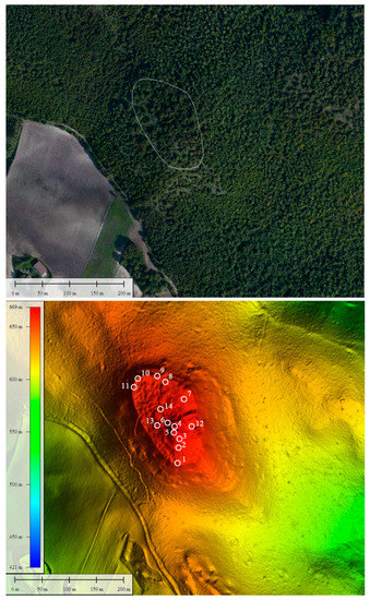
Figure 4.
Orthophoto (up) and Digital Terrain Model (DTM) (bottom) derived by LiDAR survey. In the orthophoto (up), the white line indicates the investigated area, and the numbers in the DTM (bottom) indicate the plots where field inspections were performed.
2.4. Visualization Methods: State of the Art
The LDMs aim at facilitating the analysis and interpretation of micro-topography by using diverse visualization techniques. They are generally based on how illumination is modeled for each point. There are two diverse illumination modeling: (i) direct or (ii) diffuse illumination. The direct illumination-based models represent relief features well.
The simplest technique is Hill shading (HD), which consists of illuminating the relief, considered a Lambertian surface, with an artificial light source at given zenith and azimuth angles, thus providing the shape of the terrain in a realistic fashion (e.g., [10]).
However, HD presents some drawbacks such as the identification of details in deep shades and inability to properly visualize linear features parallel to the light beam. Such drawbacks can be overcome by changing the direction of the light source or considering more directions (8, 16, and more) and/or computing the Principal Component Analysis (for archaeological applications of PCA of HD the reader is referred to [40]). The advantage of PCA is the removal of the redundancy. However, it does not provide consistent results with different datasets, because from a statistical point of view, the PCA results depend on the specific dataset under processing. These drawbacks can be overcome using diffuse illumination. This assumes that the more exposed points receive more diffuse light and appear brighter than the deeper points and, in turn, it captures relief detail in a “three-dimensional view”, assuming that the diffuse illumination is isotropic.
The diffuse illumination in computer graphics is generally called ambient occlusion and was recently presented by Yokoyama et al. [41] as “Openness” in the case of DEM visualization techniques (see also [13]). Sky-View Factor is one of the most common visualization techniques based on diffuse illumination [12]. SVF quantifies ‘the portion of the sky visible from a certain point’ within a certain radius ([12]; p. 266), in other words, large SVF denotes a large portion of the sky visible and the size of the observed area, defined by the chosen radius, influences the result. A small radius is required (e.g., 10–15 m) to highlight subtle and small-scale micro-relief as expected in Torre di Cisterna.
When almost the entire hemisphere above the pixel is visible, the SVF value is 1, as in the case of peaks and ridges; SVF is close to 0 where almost no sky is visible (bottom of deep valleys).
The main differences between SVF and Openness are the following. (i) SVF considers a homogeneous illumination from all directions above; whereas Openness considers homogeneous illumination from all directions; (ii) SVF is a physical quantity indicating the portion of the sky visible and for this reason is also used in energy balance studies; (iii) SVF uses only zenith angles above the horizontal plane (SVF can be a zenith of 90°), whereas Openness also includes larger angles. This means that for a given location, SVF delineates mainly concave features and maintains slope visibility, thus preserving the perception of general topography; whereas Openness loses slope visualization to enhance local micro-topography. SVF is particularly suitable for the visualization of depressions, such as hollow ways or mining traces, whereas positive openness highlights convexities, namely ridges and crests. Openness can also be obtained using nadir angles, and in this case is able to mark concavities and the deepest parts.
Similar to SVF is the anisotropic (directional) Sky-View Factor (ASVF) [12,42]. Both SVF and ASVF are expected to enhance visibility of simple as well as complex small-scale features whatever their orientation and shape on most types of terrain.
All the visualization techniques based on direct (HD) or diffuse (SVF) illumination can exhibit some problems in the identification of small scale features in steep land surfaces. This problem can be overcome using Local Relief Model or Trend Removal (LRM) which consists of filtering the terrain surface out, leaving just the archaeological features and their relative elevation above or below the terrain [8]. In this way, it enhances the visibility of small-scale and shallow topographic features removing large-scale landscape forms from the LiDAR data set. In particular, the LRM approach is based on the (i) smoothing of DEM by applying a low pass filter, (ii) its subtraction to the initial DEM, and (iii) calculation of the zero meter contours from the difference model to obtain break lines, as well as the intersection of the break lines with the DEM. LRM computation, as with openness, is based on the use of a kernel to obtain the statistical parameters and the results strongly depend on the kernel selection. Therefore, it must be considered that LRM can be interpreted correctly only when taking the computation process into consideration (see also [37]). The main advantage of LRM is (i) to provide immediately perception and discrimination of sunken from raised features, and (ii) to measure height differences between individual features and the surrounding area.
Finally, an alternative way to emphasize micro-topography without lighting the digital models is to compute slope gradient and convexity, which are the first and second derivative of DEM, respectively. These methods are particularly effective for digital models with high resolution and accuracy and need additional information for their interpretation.
Performances obtained from the above LDMs have been assessed by several authors. In particular, Bennett et al. [43], quantitatively compared diverse visualization techniques (LRM, SVF) for a study area in the UK. Outputs, in terms of visibility of feature length from these diverse approaches, were compared with ancillary information. Keith Challis et al. [44] discussed the strengths and weaknesses of each technique and set up a generic toolkit, ad hoc suited for the visualization of airborne LiDAR data for archaeological purposes. Finally, Mayoral et al. [45] proposed an analytical method for the assessment of the efficacy of visualization techniques using gradient modelling and spatial statistics.
All the studies suggested a combination of diverse techniques (i) to obtain a maximum amount of information extraction and facilitate the interpretation, and (ii) to face the challenge of discriminating the borderline between archaeologically induced micro-topographic variations and their surrounding surfaces. Today, several tools (for example Relief Visualization Toolbox (RVT) [46] and LiDAR-Visualisation Toolbox (LiVT) [47]) are available in commercial GIS (ArcGIS) and open source software as GRASS and QGIS. The RVT Toolbox has been used herein for the Cisterna case study.
2.5. Methodology
For the purpose of our analyses, as suggested from all the studies summarized in Section 2.4, all the diverse LDMs were used. This was done in order to obtain maximum information and to compare the performance of the diverse LDMs from both subjective (through visual inspections) and objective analyses (through automatic classifications). To improve the discrimination/extraction capability of archaeological micro-relief, noise filtering was performed as a preliminary step before the application of the most common visualization techniques (see Section 2.5.1).
The automatic feature extraction adopted herein (see Section 2.5.2) is based on an object-oriented approach suitable for the identification and extraction of subtle signals linked to the presence of buried and shallow archaeological remains, as already applied in Hierapolis [48]. Finally, the reconnaissance of archaeological features has been performed by field surveys aimed at verifying the archaeological interests of micro-relief.
The flowchart of data processing chain is showed in Figure 5 and described in Section 2.5.1, Section 2.5.2 and Section 2.5.3.
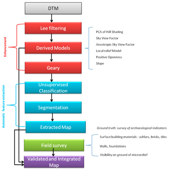
Figure 5.
Flowchart of the methodological approach.
2.5.1. Enhancement
The enhancement procedure is composed of two steps: (i) noise reduction applied to DTM; and (ii) derived models obtained from the diverse visualization techniques.
(i) The noise reduction has been performed because some LDMs with particular reference to SVF, ASVF, and Openness are generally noisy (with this respect see Mayoral et al. [45]). For this reason, it is necessary to use filtering. For the LDMs of Cisterna, Lee filtering [49] has been adopted. It replaces each given pixel value with the average (or weighted average) computed over a given window ad hoc sized to suppress noise preserving image sharpness and detail. As expected, the smaller the window size, the greater the improvement in the visualization of the micro-topographical reliefs. For this reason, we adopted a window size of 3 × 3. Figure 6a–f shows the result of Lee filtering observed on the diverse products of SVF. In particular, the filtering out of high frequencies produces a smoothing effect which makes the reconnaissance and mapping of edges of micro-topographic relief easier. Figure 6e,f evidences the added value of the Lee filter for the visualization of two different micro-topographical features (x and y in Figure 6g) that are attributable to the tower castle and (probably) a building, respectively. The first (x) is characterized by a bigger height difference compared to the second one (y), as evidenced by the profiles (X-X and Y-Y, respectively).
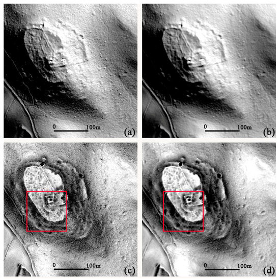
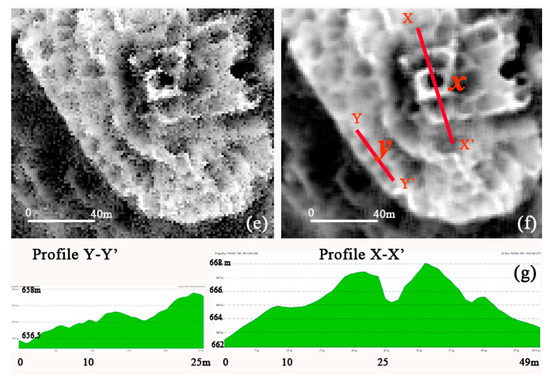
Figure 6.
Noise reduction of DTM using an enhanced Lee filter. In particular: (a) is the DTM; (b) is the DTM filtered using Lee algorithm; (c) is the result of SVF applied to DTM; (d) is the result of SVF applied to filtered DTM; (e,f) are zooms of (c,d), respectively, in the surrounding of the quadrangular landform related to the castle; (g) profiles X-X′ and Y-Y′ (see image f): the first profile crosses microrelief attributable to two buried buildings, the second one crosses the landforms attributable to the castle of Cisterna, including a square tower.
(ii) For the purpose of this study, the following visualization techniques have been adopted: PCA of Hill Shading (PCA_HD), Local relief Model (LRM), Sky View Factor (SVF), Anisotropic Sky View Factor (ASVF), Positive Openness, and Slope (for additional details see the short overview of the state of the art in Section 2.4). The efficacy of the visualization techniques depends on a number of parameters. In particular, the computation of SVF, ASVF, and Openness is influenced by the search radius of the horizon: the larger the search radius, the more generalized the results. In contrast, a small search radius can be used to visualize and classify local morphological forms. For Cisterna, considering both (i) the size of the expected micro-relief, ranging from 1.5 to 4 m (see Figure 6g, profile Y-Y′), and (ii) the geometrical resolution of the data set about 50 cm, the search radius has been set at 5 pixels for SVF, ASVF, and Openness. Another crucial parameter to set is the number of search directions. Following similar considerations as above, for Cisterna, the value of 16 search directions was set to obtain the most effective visualization in terms of visibility of archaeological micro-topographical relief. Finally, for the computation of LRM, the parameter to be set is the radius for trend assessment, in this case the value of 10 pixels was selected to obtain the best result in terms of edge enhancement of archaeological features.
A further edge enhancement has been performed using a spatial autocorrelation (SA) analysis expected to improve the following unsupervised classification process (see Section 2.5.2), as applied for looting feature extraction [50]. To assess its impact on the data processing, two parallel processing chains were adopted: one using SA and the second without SA (see Figure 5).
There are many SA indicators generally denoted as Global and Local indicators. Herein, we adopted the autocorrelation Geary’s C [51] (expressed by Formulas (1) and (2) as global or local indicator, respectively).
where N is the total pixel number, Xi and Xj are intensity in points i and j (with i ≠ j), is the average value, wij is an element of the weight matrix.
The Local Geary statistic elaborated by Anselin [51], is in Formula (2),
where the symbols have the same meaning as in Equation (1).
For digital images, global indicators provide one value which indicates the magnitude of spatial association, whereas the local indicators provide a new image that provides a measure of autocorrelation around a given pixel. Local indicators are able to identify discrete spatial patterns that may not otherwise be apparent by global statistics. For the purpose of our investigations, we used local Geary’s C indicator because is able to identify edges and areas characterized by a high variability and it is suitable to capture and uncover hidden, local patterns.
2.5.2. Automatic Feature Extraction
Automatic feature extraction (AFE) has been applied to LDMs, filtered with Lee algorithm, with and without SA based on Geary index. It is based on an object-oriented approach, suitable for the identification and extraction of subtle signals linked to presence of buried and shallow archaeological remains [48].
Object-oriented approaches are usually based on two main steps: (i) first the segmentation, (ii) then the classification. Herein, as in Lasaponara et al., 2016 [48], we firstly performed the unsupervised classification step and then the segmentation. The choice is given by the specificity of archaeological issue. In particular, the subtle features/targets to be identified are partially or totally unknown. Therefore, to cope with this issue, the first step is based on unsupervised classification, which provides a first ‘rough’ categorization of pixels, followed by the segmentation to extract the geometric shape of the previously clustered pixels. Unsupervised classification requires limited human intervention in setting up the algorithm parameters. The importance of applying unsupervised classification in archaeological applications is that: (i) it is an automatic process, namely, it usually requires only a minimal amount of initial input compared with a supervised data set; (ii) classes do not have to be defined a priori; (iii) unknown feature classes may be discovered.
A number of unsupervised classification algorithms are commonly used in remote sensing, including (i) K-means clustering, and (ii) ISODATA (Iterative Self-Organizing Data Analysis Technique) [52] which are quite similar, but ISODATA is considered more flexible compared to the K-means method and, therefore, was selected for this study.
The result of the classification is a map with a number of classes, among which one better represents the features to be extracted. They were selected for the following segmentation step to obtain meaningful feature classes. To this aim, it is also fundamental to set some parameters in order to optimize the ratio between target (features) and false alarms. The most important parameters to set are (i) the minimum population (i.e., the minimum number of pixels that must be contained in a segment) and (ii) the number of neighbors. These parameters were set as 40 and 4, respectively.
2.5.3. Reconnaissance of Archaeological Features and Validation
After the automatic identification and mapping of the features, field surveys were conducted in order to verify the archaeological interest of the identified features. Three conditions were set and considered the: (i) presence of walls and foundation remains; (ii) presence of concentrations of surface building materials, such as ashlars, bricks, tiles, pottery; (iii) visibility on ground of micro-relief along with the presence (even scattered) of surface building materials.
At least one of the three conditions had to be met to confirm the archaeological interest of features detected using LiDAR DTM and relative elaborations.
3. Results and Discussion
For the purpose of our investigations in Torre di Cisterna, all the LDMs mentioned in Section 2.5.2 have been applied to enhance the topographical relief of archaeological interest. The detected features are related to micro-relief and earthworks located on the hilly plateau at a height ranging from 656 m to 668 m asl. The plateau has an elongated oval shape, oriented in the NW–SE direction, with an area around 2.3 hectares, completely covered by oak trees and a thick undergrowth made of small trees and bushes (see orthophoto in Figure 4a).
3.1. Visual Inspections of LDMs: Results and Discussion
Figure 7 shows the results from PCA of Hill Shading, LRM, SVF, ASVF, Positive Openness, and Slope.
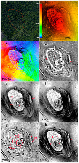
Figure 7.
Archaeological feature enhancement from LiDAR and derived Models. (a) Orthophoto: the red line indicates the investigated area; (b) DTM Lee filtered; (c) RGB of PCA of Hill Shading; (d) Simple Local relief Model; (e) Sky View Factor; (f) Anisotropic Sky View Factor; (g) Positive Openness; (h) Slope. The lettering is referred to some topographical relief discussed in the text, in particular, w1 and w2 (in d) are related to potential city walls and extramural walls, c is the castle, b refers to potential buried buildings, l refers to potential streets of the village.
At a quick comparative glance, a microtopography attributable to shallow remains of a village including fortified structures emerges. Furthermore, the LDMs show different results in terms of feature visibility from both the quantitative (number of identifiable features) and qualitative (feature discrimination) point of view.
Some of these features are easily recognizable from all the LDMs, as in the case of the quadrangular landform at south east of the hilly plateau (see c in Figure 7d,e,g,h) which is reasonably attributable to a tower-castle as expected on the basis of the information recorded by the historical topographic maps reported in Figure 2a–c. Moreover, all the LDMs clearly show microrelief bordering the edges of the plateau (see w1 in Figure 7d,e,g,h) and some linear features North east of the hill (see l in Figure 7d,g,h). The first are probably city walls, whereas the second may refer to possible urban streets.
Finally, all the other features, representing the greatest amount of microrelief, refer to potential shallow structures of buildings (see b in Figure 7e,g), which are less visible and more difficult to recognize and interpret compared to the bigger features of the castle and the potential city walls.
For these subtle features, a significant enhancement in terms of feature visibility has been obtained in particular by SVF, Openness, and ASFV (see Figure 7e–g, respectively)
However, all the LDMs are complementary for their diverse capability to emphasize the micro-topographical features. For example, the slope map shows, in an effective way, the quadrangular landform, bringing out the fortified structure (see c in Figure 7h). Also, the linear features l (showed in Figure 7h) are very well imaged by the slope map, thus suggesting that they would be urban streets. Both the LRM and PCA_HD (see Figure 7c,d), even if quite limited in imaging small features, display the quadrangular feature w2 at the east of the potential city well, thus suggesting the presence of extramural walls (see also w2 in Figure 7e,g,h).
As a whole, the best results are obtained from SVF, ASVF, and Openness especially for the smaller features (see b in Figure 7e,g and bi in the map of Figure 8) of shallow buildings and urban blocks. Moreover, compared to LRM and Slope, they provide additional details of earthworks and landforms attributed to the tower castle and walls.
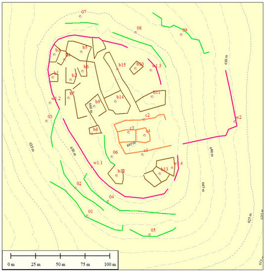
Figure 8.
Reconnaissance and mapping of archaeological features on the basis of the integration of the features obtained from all the considered LDMs.
The integration of the features observed from all the LDMs (showed in Figure 7c–h) allowed the identification and mapping of all the potential microrelief of archaeological interest (see map in Figure 8). Four types of features have been identified. They are: (i) earthworks of possible city walls (w1.i) and an extramural wall (w2), (ii) landform and microrelief of the castle, (iii) micro-topographical relief probably related to buried buildings and streets of the new discovered village (indicated with bi in Figure 7), and finally, (iv) other features of potential anthropogenic origin (denoted with oi)
A qualitative assessment of the feature visibility of LDMs (see Figure 8) has been performed by visual inspection. The reconnaissance of the features has been facilitated by the field survey (see Figure 9) conducted to verify the cultural interest of landforms. The forest of oaks with dense undergrowth made the survey very difficult and, in many cases, the areas to be surveyed were inaccessible. Furthermore, most of the potential microrelief identifiable from the LDMs is not easily visible on the ground. However, the in situ observation allowed us to map the presence of materials, such as brick roof tiles, fragments of bricks, and worked stones, which helped us in the interpretation of the remotely-sensed archaeological features. The following two criteria were adopted for selecting the areas for the in-situ inspections: (a) the presence of microtopographical variations visible from LiDAR-based maps and profiles; and (b) the accessibility. As a whole, 15 areas (showed in Figure 4) representative of the diverse types of archaeological features, such as microrelief attributable to shallow buildings and landforms related to the castle and city walls, were inspected and measured by GPS.
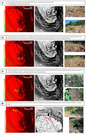
Figure 9.
In situ inspections of microtopographical variations observed from LiDAR DTM and derived models. The image shows DTM, Sky View factor results, and some photos of the four plots named 1, 3, 5, and 8.
The field survey was conducted in order to identify the following archaeological indicators: (i) walls, wall foundations, and stone material of collapsed masonry structures; (ii) building surface materials, such as worked stones, bricks, and roof tiles; (iii) visible and surveyable microrelief (including earth works) along with surface building materials.
The existence of one of the three above said indicators has been considered enough for the ‘archaeological validation’ of the features identified from LDMs. Figure 9 shows four areas surveyed, named 1, 3, 5, and 8. They are related respectively to city walls (1), the castle (3), the tower (5), and an area including a road and a urban block (8). In (1), the archaeological indicators were earthworks and sparse building materials, including worked stones, bricks, and tiles. In (3), sparse building materials and remains of collapsed walls were observed. In (5), remains of walls of height ranging from 40 to 120 cm were measured. The masonry is composed of slightly carved stone blocks, complemented with small ashlars and fragments of bricks laid in place on more or less regular horizontal rows. Finally, in (8), sparse building materials including bricks and tiles were observed.
As previously said, the assessment of archaeological feature visibility from the diverse LDMs has been conducted by six of the coauthors: two experts in remote sensing archaeology (N.M. and R.L.), one archaeologist (A.P.), one historian, an expert in conservation (M.B.), and two geologists (F.T.G. and M.S.).
The assessment has been performed comparing features xi (w1.1, w1.2...b1, b2, b3..., o1, o2, o3 see Table 2) mapped (xiFM) in Figure 8 with the features visible from the single derived model (xiFDM).
Table 2.
Assessment of archaeological feature visibility from the diverse derived models (PCA_HD, LRM, SVF, ASVF, Openness, Slope). Legend. xi archaeological features; LDM: LiDAR Derived Models (PCA_HD, LRM, SVF, ASVF, Openness, Slope); w1.1, w1.2...b1, b2, b3..., o1, o2, o3... are the features of potential archaeological interest identified and mapped (see Figure 7) on the basis of the diverse LDMs; LFM: length of features (w.1.1...b1...o1...etc.) mapped (see Figure 7); LFDM length of features from the LDMs; µxi (µPCA, µLRM, µSVF, µASVF, µOpen, µslope) are the normalized visibility indices of features from the diverse LDMs expressed by LxiFDM/LxiFM; Lw, Lb, Lc, Lo: total length of archaeological features attributed to city walls, buildings, castle, and other, respectively (Lw′, Lb′, Lc′, Lo′): total length of archaeological features validated by ground truth; µLDM is the weighted average of µxi for a given LDM expressed by the following formula ΣLxFDMi*µxi/ΣLxFMi; µLDM′ is the same of µLDM but computed considering only the features xi which have been validated (GDV = y); GDV: ground-truth validation (Y: yes; N: no); GDR: Ground truth result (w: walls, remains of walls, and foundations; sb: surface building materials (stones, bricks, tiles); m: microrelief and earthworks visible on ground, No: no result from Ground truth validation).
Furthermore, the normalized visibility index shown in Formula (3) has been computed for the diverse LDMs.
where µxi is normalized visibility index for the given LDMs reported in Table 2 (µiPCA, µiLRM, µiSVF etc.); LxiFDM is the length of the feature xi visible from a given LDM; LxiFM is the length of xi as mapped in Figure 8.
µxi = LxiFDM/LxiFM
Table 2 lists the features xi grouped for 4 classes related to city walls (wi), the castle (ci), small microrelief attributed to potential buried buildings or streets of the urban fabric (bi), and other features of potential archaeological interest (oi). For each class and each derived model, the weighted average of normalized visibility index µLDM has been computed according to Formula (4).
where the parameters are the same as in Formula (3). This index has been also computed for the features validated in situ: in this case the index is named µLDM′.
µLDM = ΣLxiFDM*µxi/ΣLxiFM.
As whole, Table 2 lists 33 features, also drawn in the map of Figure 8, attributable to city walls (wi), the castle (ci), the urban blocks and buildings (bi), and other features (oi) of the medieval village. In Table 2, column GDV indicates the LDMs-based features xi inspected in situ and the GDR column reports the results of the in situ survey (presence of walls, surface building materials etc.).
In particular, with respect to city walls, n.5 features were recognized from the LDMs for a total length of 469 m, among which n.3 features were observed and validated on the ground for a total length of 413 m. They were characterized by microrelief, building surface materials (w1.1, w1.2), and remains of walls (w2). The other features (wi.3 and w1.4) were not inspected due to the dense vegetation.
For all the LDMs, the normalized visibility index (µLDM′) exhibits values ranging from 0.85 to 0.98. In particular, higher values (0.95 to 0.98) were obtained for LRM, SVF, ASVF, and Openness, and slightly lower values for PCA_HD and Slope (0.85 and 0.91, respectively).
Similar values have been obtained also considering the features inspected on the ground (see µLDM and compare with µLDM′ in Table 2).
In the area of the castle, n.5 features visible from the LDMs have been all inspected. The inspection revealed some walls, microrelief, and a great amount of building materials, such as ashlars, bricks, tiles, and pottery (see column GDV and GDR of Table 2). Moreover, the comparative assessment put in evidence higher values of µLDM for SVF, ASVF, and Openness (µLD = 1) with respect to PCA_HD, LRM, and Slope (equal to 0.54, 0.72 and 0.74, respectively).
For small features (bi), the µLDM values obtained from SVF, ASVF, and Openness were much higher than those PCA_HD, LRM and Slope: 0.97 to 1 versus 0.40 to 0.66, respectively (see also Figure 9). This difference is significantly reduced considering only the features inspected (0.98 to 1 for SVF, ASVF, and Openness, versus 0.73 to 0.89 for PCA_HD, LRM and Slope). In this case, the vegetation cover density played a fundamental role; in fact, where it was possible to inspect the microtopographical features, the vegetation cover was less dense and, consequently, was characterized by a higher ground return density with a better visibility of microtopographical changes. A similar behavior has been found for the class of other archaeological features (see histograms in Figure 10).
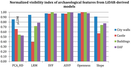
Figure 10.
Histogram: normalized archaeological feature visibility from the diverse LiDAR-derived models.
As a whole, the different performance of the LDMs is due to the fact that the diffuse illumination-based models (SVF, ASVF, and Openness) enhance the edges better than the other methods (PCA of Hill Shading, Slope, LRM). This is particularly evident for small features. The histograms in Figure 10 show that, considering the entire set of LDMs, the best results in terms of feature visibility have been obtained for the city walls and the castle because they were characterized by greater dimensions, more durable construction materials, and were abandoned later compared to buildings of the village.
3.2. Automatic Feature Extraction: Results and Discussion
Automatic feature extraction (AFE) was performed using ISODATA and segmentation, described in Section 2.5.2 (see also flowchart in Figure 5), applied with and without Local Geary index, to assess its impact on the data processing chain. The use of Local Geary index has been successfully used for extracting archaeological looted areas in Syria and in Peru [44]. Results from AFE performed for all the LDMs, with and without of the use of Geary index, generally provided only bigger features related to castle and city walls. In order to compare the performance obtained from the diverse LDMs, the outputs from the automatic feature extraction have been compared with the map in Figure 8 and field surveys.
For sake of brevity, we only show and discuss the results of AFE obtained from SVF, Positive Openness, and the Local Relief Model. Figure 11 depicts the partial and final results of AFE.
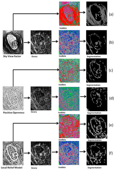
Figure 11.
Results of automatic feature extraction without and with Geary index applied to SVF (a,b, respectively), Positive Openness (c,d, respectively), and Local relief Model (e,f, respectively).
The AFE method without Geary presents a very good result from Positive Openness; whereas LRM extracts a large part of the ‘big’ features but with a high number of commission errors. Finally, for SVF, AFE extracts only some structures of the castle and sloping surface of the hill.
The use of Geary before ISODATA allowed significant improvement in the extraction of archaeological features, with a result comparable with that obtained from Openness without Geary. On the other side, with respect to Openness, the use of Geary does not provide any improvement but tends to add commission errors. Similarly, Geary, when applied to LRM, reduces the number of pixels extracted, thus losing the spatial continuity of archaeological features.
The difference in the results with and without Geary for the diverse LDMs can be explained on the basis of their different enhancement behaviors. In particular, positive openness is devised to identify and thin edges that tend to be degraded after Geary because it detects areas of dissimilarity and areas characterized by a high variability compared to the values of its neighboring pixels, thus: (i) ‘loosing pixels’ along the archaeological features of walls and castle already highlighted by Openness, and (ii) adding commission errors, particularly North and Northeast of the plateau.
While SVF mainly delineates concave features and maintains the visibility of the slope, it offers more margins of improvement in the enhancement of local microtopography; for this reason, the use of Geary, detecting dissimilarity and high variability, enabled us to sharpen microtopographical changes. AFE takes advantage of this, providing suitable extraction of archaeological features.
Figure 12 resumes the results of AFE obtained from SVF and Openness, with and without Geary, respectively, which have been compared by overlaying both of them with the map in Figure 8. The comparison (see Table 3) shows a rate of success (RS) ranging from 81 to 97% for the castle and city walls, with no significant difference between Openness (RS equal to 86% and 93% for the castle and city walls, respectively) and SVF (RS equal to 83% and 97%, for the castle and city walls, respectively).
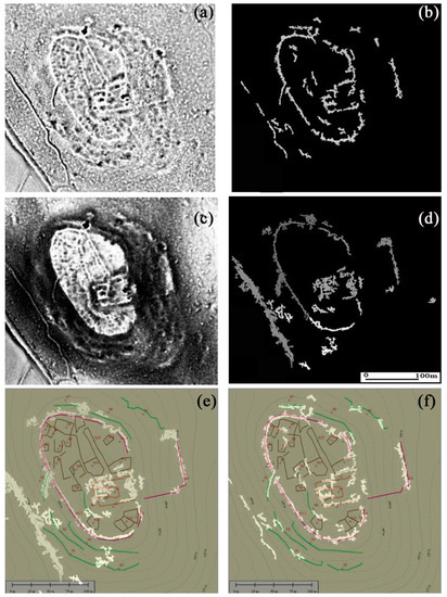
Figure 12.
Automatic feature extraction (AFE): comparison of the results obtained by applying AFE to Openness and SVF. In particular: (a,b) are positive openness map and the result of AFE, respectively; (c,d) are SVF map and the result of AFE, respectively; (e,f) depict the image (b,d) on the map in Figure 8.
Table 3.
Assessment of AFE applied to Sky View Factor and Positive Openness (see Figure 11e,f, respectively).
The main difference in the performance from AFE applied to Openness and SVF is evident for the smaller features, such as buildings and other archaeological features: the values of RS obtained for Openness are 14% and 34%, respectively, compared to 4% and 20%, respectively, for SVF.
3.3. Archaeological Result: Brief Considerations
From the archaeological point of view, the main LiDAR-based result, validated by field surveys, has been the re-discovery of the remains of a medieval castle under a dense canopy, documented by a few historical sources and some historical maps (see Section 2.1) and the discovery of other structures completely unknown before our investigations, such as the walls bordering the hill and buildings of the habitation area.
The main architectural characteristics for both the castle and the village (see Figure 13) are known thanks to the use of LiDAR and, in particular, to LiDAR-derived models based on diverse visualization techniques.
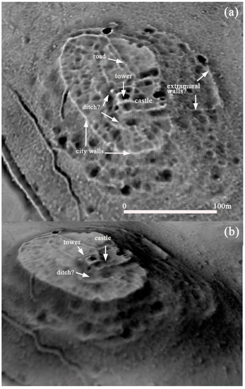
Figure 13.
SVF map (a) and 3D visualization (b) with archaeological interpretation.
The castle is a 13-m-high square tower surrounded by a square fence and was probably protected by a ditch. This structure is very similar to other coeval castles, such as Monte Serico in Basilicata [53,54], Tertiveri and Castel Fiorentino in Apulia [24], Termoli in Molise [55], located quite close to Cisterna, all of which were founded in the Norman age (12th century) and later (13th century) enlarged and restored during the age of Emperor Frederick II. They are all characterized by a typology named ‘pyramidenturm’ by the German archaeologist Haseloff [55] which was one of the constructive types of fortified architecture in Southern Italy between the 12th and 13th centuries.
The obtained maps depict the presence of extramural walls which denote the importance of this settlement built at the beginning of the 11th century to play an important role in the control of the territory, being a strategic position close to a lime (i.e., frontier) separating and protecting the frontiers between Byzantine and Longobard territories. For this reason, it was conceived to be a ‘civitas’, an episcopal seat and, consequently, was inhabited by a significant number of people for the time. This would explain the several microtopographical relief features attributable to shallow buildings identified by means of Openness, SVF, and ASVF.
Historical sources do not allow us to add anything else. Starting from the results of these LiDAR-based investigations, future archaeological research will shed light on the events of this fortified settlement and its castle from its foundation to abandonment
4. Conclusions
This study brings to light a medieval fortified site completely covered by dense vegetation and little documented, using LiDAR surveying and diverse derived models which have been integrated and compared to obtain maximum information. The site is Torre di Cisterna, located at North of Melfi (Southern Italy), in a strategic position between the Longobard and Byzantine frontiers at the beginning of the 11th century.
The paper enables us to advance in both technological and archaeological domains. From the technological point of view, by using subjective and objective approaches, the diverse derived models have been tested to assess their capability in surveying the microtopography of a site of archaeological interest covered by a dense canopy and understory vegetation. For the first time, an object-oriented approach based on spatial autocorrelation, unsupervised classification, and segmentation, has been used limit the human intervention in LiDAR data processing. The use of automatic feature extraction procedures is very attractive when using a large LiDAR dataset (as today available from several institutions) for a high number of potential hilly medieval sites under canopy.
The results observed from the archaeological perspective are very exciting. The LiDAR-based approach allowed us (i) to discover a medieval village for which very little information is available from historical sources, and (ii) to cast new light on a fortified complex, dated to Emperor Frederick II, for which only the existence of a tower was known.
The results were validated by in situ analyses, which demonstrated that the automatic procedure can detect and extract the main distinctive features of medieval settlements, such as castle and city walls. Smaller features, attributable to buried structures of habitation area, are better identifiable by visual inspection of LiDAR-derived models based on Sky View Factor, Anisotropic Sky View Factor, and Openness.
This paper opens new perspectives for the study of lost medieval villages, a topic of great interest for several reasons, among which are investigating (i) the role of climatic and environmental changes or natural disasters in their decline; (ii) the study of diverse resilience strategies in crisis periods such the Late Middle Ages; (iii) the importance of enhancing this rich cultural heritage still preserved in the subsoil and in many cases under canopy; (iv) the exciting challenge from the scientific and archaeological point of view which impose ad hoc approaches by using remote sensing technologies based on LiDAR and automatic classification of archaeological features as in Ref. [56].
Author Contributions
N.M. conceived and directed the investigations, coordinated the drafting of the paper, conducted LiDAR data processing, developed remote sensing-based methodology with R.L., wrote along with R.L. Section 1, Section 2.2, Section 2.3, Section 2.4, Section 2.5, Section 3 and Section 4. F.T.G. co-directed the investigations, coordinated in-situ-analyses, contributed to Section 2.1 and Section 3.1. M.B., Mi.S. (Michele Sedile), V.F. contributed to the historical research and Section 2.1. Ma.S. contributed to in-situ analyses, conducted GPS measurements and Section 2.1. A.P. contributed to in-situ analyses. B.L. conducted LiDAR data classification and coordinated LiDAR data acquisition. R.L. revised the whole paper, developed with N.M. remote sensing based methodology, wrote along with N.M. Section 1, Section 2.2, Section 2.3, Section 2.5, Section 3 and Section 4.
Funding
This research received no external funding.
Conflicts of Interest
The authors declare no conflicts of interest.
References
- Chase, A.S.Z.; Chase, D.Z.; Chase, A.F. LiDAR for Archaeological Research and the Study of Historical Landscapes. In Sensing the Past: From Artifact to Historical Site; Masini, N., Soldovieri, F., Eds.; Springer: New York, NY, USA, 2017; pp. 89–100. [Google Scholar]
- Chase, A.F.; Chase, D.Z.; Weishampel, J.F.; Drake, J.B.; Shrestha, R.L.; Slatton, K.C.; Awe, J.; Carter, W.E. Airborne LiDAR, archaeology, and the ancient Maya landscape at Caracol, Belize. J. Archaeol. Sci. 2011, 38, 387–398. [Google Scholar] [CrossRef]
- Evans, D.H.; Fletcher, R.J.; Pottier, C.; Chevance, J.B.; Soutif, D.; Tan, B.S.; Im, S.; Ea, D.; Tin, T.; Kim, S.; et al. Uncovering archaeological landscapes at angkor using LiDAR. Proc. Natl. Acad. Sci. USA 2013, 110, 12595–12600. [Google Scholar] [CrossRef] [PubMed]
- Doneus, M.; Briese, C.; Fera, M.; Janner, M. Archaeological prospection of forested areas using full-waveform airborne laser scanning. J. Archaeol. Sci. 2008, 35, 882–893. [Google Scholar] [CrossRef]
- Fernández-Lozano, J.; Gutiérrez-Alonso, G. Improving archaeological prospection using localized UAVs assisted photogrammetry: An example from the Roman Gold District of the Eria River Valley (NW Spain). J. Archaeol. Sci. 2016, 5, 509–520. [Google Scholar] [CrossRef]
- Fernández-Lozano, J.; Gutiérrez-Alonso, G.; Fernández-Morán, M. Using airborne LiDAR sensing technology and aerial orthoimages to unravel roman water supply systems and gold works in NW Spain (Eria valley, León). J. Archaeol. Sci. 2015, 53, 356–373. [Google Scholar] [CrossRef]
- Lasaponara, R.; Masini, N.; Holmgren, R.; Backe Forsberg, Y. Integration of aerial and satellite remote sensing for archaeological investigations: A case study of the Etruscan site San Giovenale. J. Geophys. Eng. 2012, 9, S26–S39. [Google Scholar] [CrossRef]
- Hutson, S.R. Adapting LiDAR data for regional variation in the tropics: A case study from the Northern Maya Lowlands. J. Archaeol. Sci. 2015, 4, 252–263. [Google Scholar] [CrossRef]
- Prufer, K.M.; Thompson, A.E.; Kennett, D.J. Evaluating airborne LiDAR for detecting settlements and modified landscapes in disturbed tropical environments at Uxbenká, Belize. J. Archaeol. Sci. 2015, 57, 1–13. [Google Scholar] [CrossRef]
- Masini, N.; Coluzzi, R.; Lasaponara, R. On the Airborne Lidar Contribution in Archaeology: From Site Identification to Landscape Investigation. In Laser Scanning, Theory and Applications; Wang, C.-C., Ed.; Intech: London, UK, 2011; pp. 263–290. ISBN 978-953-307-205-0. [Google Scholar]
- Hesse, R. LiDAR-derived Local Relief Models a new tool for archaeological prospection. Archaeol. Prospect. 2010, 17, 67–72. [Google Scholar] [CrossRef]
- Zakšek, K.; Oštir, K.; Kokalj, Ž. Sky-view factor as a relief visualization technique. Remote Sens. 2011, 3, 398–415. [Google Scholar] [CrossRef]
- Doneus, M. Openness as visualization technique for interpretative mapping of airborne LiDAR derived digital terrain models. Remote Sens. 2013, 5, 6427–6442. [Google Scholar] [CrossRef]
- D’Archimbaud, D. Rougiers, Castrum médiéval déserté. Pays Sainte-Baume 2001, 9, 6–8. [Google Scholar]
- Simms, A. Deserted medieval villages and fields in Germany, a survey of the literature with a select bibliography. J. Hist. Geogr. 1976, 2, 223–238. [Google Scholar] [CrossRef]
- Corns, A.; Shaw, R. High resolution 3-dimensional documentation of archaeological monuments & landscapes using airborne LiDAR. J. Cult. Herit. 2009, 10 (Suppl. 1), e72–e77. [Google Scholar]
- Heine, H.W. Innovative methods for surveying castles located in forests or shallow water in Lower Saxony. [Innovative methoden zur erfassung und vermessung von burgen in wäldern und flachgewässern (Niedersachsen) CG]. Chateau Gaillard 2012, 25, 197–202. [Google Scholar]
- Lasaponara, R.; Masini, N. Full-waveform Airborne Laser Scanning for the detection of medieval archaeological microtopographic relief. J. Cult. Herit. 2009, 10, e78–e82. [Google Scholar] [CrossRef]
- Lasaponara, R.; Coluzzi, R.; Gizzi, F.T.; Masini, N. On the LiDAR contribution for the archaeological and geomorphological study of a deserted medieval village in Southern Italy. J. Geophys. Eng. 2010, 7, 155–163. [Google Scholar] [CrossRef]
- Krivanek, R. Comparison Study to the Use of Geophysical Methods at Archaeological Sites Observed by Various Remote Sensing Techniques in the Czech Republic. Geosciences 2017, 7, 81. [Google Scholar] [CrossRef]
- Simmons, I.G. Rural landscapes between the East Fen and the Tofts in south-east Lincolnshire 1100–1550. Landsc. Hist. 2013, 34, 81–90. [Google Scholar] [CrossRef]
- Baubiniene, A.; Morkunaite, R.; Bauža, D.; Vaitkevicius, G.; Petrošius, R. Aspects and methods in reconstructing the medieval terrain and deposits in Vilnius. Quat. Int. 2015, 386, 83–88. [Google Scholar] [CrossRef]
- Pedio, T. Centri Scomparsi in Basilicata; Edizioni Osanna: Venosa, Italy, 1990. [Google Scholar]
- Malatesta, A.; Perno, U.; Stampanoni, G. (Eds.) Note Illustrative Della Carta Geologica d’Italia Alla Scala 1:100,000. Foglio 175 (Cerignola); Istituto Poligrafico e Zecca dello Stato-Archivi di Stato: Roma, Italy, 1967. (In Italian) [Google Scholar]
- Calò Maria, M.S.I. “villages désertés” della Capitanata. Fiorentino e Montecorvino. In Proceedings of the XXVII National Conference on “Preistoria—Protostoria—Storia della Daunia, San Severo, Italy, 25–26 Novembre 2005; pp. 43–90. [Google Scholar]
- Sthamer, E. Die Verwaltung der Kastelle im Königreich Sizilien unter Kaiser Friedrich II. Und Karl I. von Anjou; Walter de Gruyter: Leipzig, Germany, 1914. [Google Scholar]
- Sciara, F. Ritrovate le Residenze di Caccia di Federico II Imperatore a Cisterna (Melfi) e Presso Apice; Arte Medievale Serise 2; Silvana Editoriale: Cinisello Balsamo (Milano), Italy, 1997; Volume 11, pp. 125–131. [Google Scholar]
- Fortunato, G. Badie, Feudi e Baroni Della Valle di Vitalba; Note a Fortunato, Per la Storia del Mezzogiorno d’Italia nell’età medievale Montemurro, Matera s.a. Edizione definitiva in G. Fortunato Badie feudali e baroni; Pedio, T., Ed.; Lacaita Editore: Manduria, Italy, 1968; Volume III, pp. 7–627. [Google Scholar]
- Angelini, G. Venosa e la media Valle dell’Ofanto nella cartografia antica in Formez. In La Natura e il Paesaggio in Orazio; Centro Universitario Europeo per i Beni Culturali: Ravello, Italy, 1995; pp. 37–48. [Google Scholar]
- Ardoini, P.B. Descrizione dello Stato di Melfi (1674), Introduzione e Note di Enzo Navazio, s.l.; Casa Editrice Tre Taverne: Melfi, Italy, 1980. [Google Scholar]
- Liaci Marcianese, A. Melfi nella storia e nell’economia (II). In La Zagaglia: Rassegna di Scienze, Lettere ed Arti, A. X, n. 38; Emeroteca Digitale Salentina Lecce 1968; pp. 189–202.
- Mallet, C.; Bretar, F. Full-waveform topographic LiDAR: State-of-the-art. ISPRS J. Photogramm. Remote Sens. 2009, 64, 1–16. [Google Scholar] [CrossRef]
- Hu, B.; Gumerov, D.; Wang, J.; Zhang, W. An Integrated Approach to Generating Accurate DTM from Airborne Full-Waveform LiDAR Data. Remote Sens. 2017, 9, 871. [Google Scholar] [CrossRef]
- Sithole, G.; Vosselman, G. Experimental comparison of filtering algorithms for bare-earth extraction from airborne laser scanning point clouds. ISPRS J. Photogramm. Remote Sens. 2004, 59, 85–101. [Google Scholar] [CrossRef]
- Axelsson, P. DEM generation from laser scanner data using adaptive TIN models. Int. Arch. Photogramm. Remote Sens. 2000, 33, 110–117. [Google Scholar]
- Briese, C.; Pfeifer, N. Airborne laser scanning and derivation of digital terrain models. In Optical 3D Measurement Techniques; Gruen, A., Kahmen, H., Eds.; Technical University: Vienna, Austria, 2001; pp. 80–87. [Google Scholar]
- Elmqvist, M. Ground estimation of laser radar data using active shape models. In Proceedings of the OEEPE Workshop on Airborne Laserscanning and Interferometric SAR for Detailed Digital Elevation Models, Stockholm, Sweden, 1–3 March 2001; Volume 40, p. 8. [Google Scholar]
- Soininen, A. Terrascan User’s Guide. Terrasolid: Helsinki, Finland. Available online: http://www.terrasolid.com/download/user_guides.php (accessed on 30 May 2017).
- Lasaponara, R.; Coluzzi, R.; Masini, N. Flights into the past: Full-Waveform airborne laser scanning data for archaeological investigation. J. Archaeol. Sci. 2011, 38, 2061–2070. [Google Scholar] [CrossRef]
- Devereux, B.J.; Amable, G.S.; Crow, P. Visualisation of LiDAR terrain models for archaeological feature detection. Antiquity 2008, 82, 470–479. [Google Scholar] [CrossRef]
- Yokoyama, R.; Shlrasawa, M.; Pike, R.J. Visualizing Topography by Openness: A New Application of Image Processing to Digital Elevation Models. Photogramm. Eng. Remote Sens. 2002, 68, 251–266. [Google Scholar]
- Kokalj, Ž.; Hesse, R. Airborne Laser Scanning Raster Data Visualization. A Guide to Good Practice; Založba ZRC: Ljubljana, Republika Slovenija, 2017. [Google Scholar]
- Bennett, R.; Welham, K.; Hill, R.A.; Ford, A. A comparison of visualization techniques for models created from airborne laser scanned data. Archaeol. Prospect. 2012, 19, 41–48. [Google Scholar] [CrossRef]
- Challis, K.; Forlin, P.; Kincey, M. A Generic Toolkit for the Visualization of Archaeological Features on Airborne LiDAR Elevation Data. Archaeol. Prospect. 2011. [Google Scholar] [CrossRef]
- Mayoral, A.; Toumazet, J.-P.; Simon, F.-X.; Vautier, F.; Peiry, J.-L. The Highest Gradient Model: A New Method for Analytical Assessment of the Efficiency of LiDAR-Derived Visualization Techniques for Landform Detection and Mapping. Remote Sens. 2017, 9, 120. [Google Scholar] [CrossRef]
- Relief Visualization Toolbox (RVT). Available online: https://iaps.zrc-sazu.si/en/rvt#v (accessed on 13 August 2018).
- LiDAR-Visualisation Toolbox (LiVT). Available online: http://www.arcland.eu/outreach/software-tools/1806-lidar-visualisation-toolbox-livt (accessed on 13 August 2018).
- Lasaponara, R.; Leucci, G.; Masini, N.; Persico, R.; Scardozzi, G. Towards an operative use of remote sensing for exploring the past using satellite data: The case study of Hierapolis (Turkey). Remote Sens. Environ. 2016, 174, 148–164. [Google Scholar] [CrossRef]
- Lee, J.-S. Digital Image Enhancement and Noise Filtering by Use of Local Statistics. IEEE Trans. Pattern Anal. Mach. Intell. 1980, 2, 165–168. [Google Scholar] [CrossRef] [PubMed]
- Lasaponara, R.; Masini, N. Space-Based Identification of Archaeological Illegal Excavations and a New Automatic Method for Looting Feature Extraction in Desert Areas. Surv. Geophys. 2018. [Google Scholar] [CrossRef]
- Anselin, L. Local Indicators of Spatial Association LISA. Geogr. Anal. 1995, 27, 93–115. [Google Scholar] [CrossRef]
- Ball, G.H.; Hall, D.J. ISODATA, a Novel Method of Data Analysis and Pattern Classification; Stanford Research Institute: Menlo Park, CA, USA, 1965. [Google Scholar]
- Masini, N. Dai Normanni agli Angioini: Castelli e Fortificazioni della Basilicata; Storia della Basilicata. Il Medioevo; Fonseca, C.D., Ed.; Editori Laterza: Roma, Italy, 2006; pp. 689–753. ISBN 8842075094. [Google Scholar]
- Lasaponara, R.; Masini, N. QuickBird-based analysis for the spatial characterization of archaeological sites: Case study of the Monte Serico Medioeval village. Geophys. Res. Lett. 2005, 32, L12313. [Google Scholar] [CrossRef]
- Haseloff, A. Die Bauten der Hohenstaufen in Unteritalien; KW Hiersemann: Leipzig, Germany, 1920. [Google Scholar]
- Lipo, C.P.; Sanger, M.; Davis, D. Automated mound detection using LiDAR and object-based image analysis in Beaufort County, SC. Southeast. Archaeol. 2018, 37. [Google Scholar] [CrossRef]
© 2018 by the authors. Licensee MDPI, Basel, Switzerland. This article is an open access article distributed under the terms and conditions of the Creative Commons Attribution (CC BY) license (http://creativecommons.org/licenses/by/4.0/).