Article

AMSR2 Soil Moisture Downscaling Using Temperature and Vegetation Data

1
School of Earth Ocean and Environment, University of South Carolina, Columbia, SC 29208, USA
2
Hydrological Sciences Branch, NASA Goddard Space Flight Center, Greenbelt, MD 20771, USA
3
Hydrology and Remote Sensing Laboratory, Beltsville Agricultural Research Center, United States Department of Agriculture, Beltsville, MD 20705, USA
*
Author to whom correspondence should be addressed.
Remote Sens. 2018, 10(10), 1575; https://doi.org/10.3390/rs10101575
Submission received: 16 July 2018 / Revised: 11 September 2018 / Accepted: 20 September 2018 / Published: 1 October 2018

Abstract

:
Soil moisture (SM) applications in terrestrial hydrology require higher spatial resolution soil moisture products than those provided by passive microwave remote sensing instruments (grid resolution of 9 km or larger). In this investigation, an innovative algorithm that uses visible/infrared remote sensing observations to downscale Advanced Microwave Scanning Radiometer 2 (AMSR2) coarse spatial resolution SM products was developed and implemented for use with data provided by the Advanced Microwave Scanning Radiometer 2 (AMSR2). The method is based on using the Normalized Difference Vegetation Index (NDVI) modulated relationships between day/night SM and temperature change at corresponding times. Land surface model output variables from the North America Land Data Assimilation System (NLDAS), remote sensing data from the Moderate-Resolution Imaging Spectroradiometer (MODIS), and Advanced Very High Resolution Radiometer (AVHRR) were used in this methodology. The functional relationships developed using NLDAS data at a grid resolution of 12.5 km were applied to downscale AMSR2 JAXA (Japan Aerospace Exploration Agency) SM product (25 km) using MODIS land surface temperature (LST) and NDVI observations (1 km) to produce the 1 km SM estimates. The downscaled SM estimates were validated by comparing them with ISMN (International Soil Moisture Network) in situ SM in the Black Bear–Red Rock watershed, central Oklahoma between 2015–2017. The overall statistical variables of the downscaled AMSR2 SM validation R2, slope, RMSE and bias, demonstrate good accuracy. The downscaled SM better characterized the spatial and temporal variability of SM at watershed scales than the original SM product.

1. Introduction

Satellite technology is a practical approach to monitoring Earth surface hydrological characteristics especially in regions with limited ground measurements [1,2,3,4,5,6,7,8]. Studies have shown that passive microwave satellite sensors can provide reliable estimates of surface SM [9,10,11,12]. Current low frequency (L-band to X-band) passive radiometers in space provide SM with intrinsic spatial resolutions of ~25–40 km. Data are often interpolated or resampled to grids with higher resolutions (9 km for the Soil Moisture Active Passive (SMAP) mission). These products are valuable for some applications but cannot satisfy all hydrological, agricultural, and weather applications. In contrast, satellite-based radars have much higher spatial resolutions but have limited spatial coverage and infrequent temporal revisit. In addition, SM retrievals from radars are more complex than from radiometers. The spatial variability and sensitivity of active and passive microwave remote sensing SM at different resolutions has been reported in [13,14,15,16].
Passive SM products are available from several sources and satellites that include the AMSR-E (Advanced Microwave Scanning Radiometer for the Earth Observing System) and its successor AMSR2, as well as SMOS (Soil Moisture and Ocean Salinity), Aquarius, and SMAP (Soil Moisture Active Passive). Here we focus on SM retrieved from the AMSR2 instrument. The AMSR2 instrument on board GCOM-W [17,18,19] was launched on 18 May 2012 by JAXA. It has six different frequency microwave bands ranging from 6.925 to 89 GHz (C, X, Ku, and Ka bands), recording the emitted microwave energy from the Earth surface at an altitude of 700 km every 1–2 days [20]. Several research groups produce AMSR2 SM products using different algorithms [21], including the JAXA soil moisture algorithm [22], Single Channel Algorithm (SCA) [23], and Land Parameter Retrieval Model (LPRM) [24].
SM downscaling algorithms attempt to produce higher spatial resolution SM data by integrating coarse-resolution passive microwave SM (or brightness temperature) with high-resolution data from other sources. Several different types of methods have been proposed and evaluated. One type of method utilized high spatial resolution radar backscatter data to downscale coarse resolution radiometer observations [25,26,27,28]. The downscaling algorithm of [29,30] used a functional relationship between brightness temperature and backscatter for each pixel based on a time series of observations. In addition to the type of methods mentioned above, other techniques, including data assimilation and machine learning, have been used to develop SM downscaling algorithms [31,32,33,34,35,36].
Besides the above two types of methods, a number of SM downscaling approaches using high spatial resolution visible/infrared band remotely sensed products have been explored in previous studies. In these approaches, the relationship between SM and soil evaporation efficiency was used to downscale SMOS SM [37,38,39] using two SM indices: Evaporative Fraction (EF) and Actual Evaporative Fraction (AEF) [40]. Fang et al. [41] developed a variant of this approach and downscaled AMSR-E SM using NLDAS model outputs. Other methods proposed include a downscaling algorithm derived from MODIS NDVI, LST, and brightness temperature, which has been applied to SMOS SM [42], a downscaling model based on vegetation temperature index [43], synergistic approaches using MODIS NDVI and LST to downscale AMSR-E and SMOS SM [44,45], and, using the thermal inertia relationship between daily average SM, temperature variation and NDVI to downscale passive microwave SM from AMSR-E and SMOS in Oklahoma [46,47,48].
The downscaling algorithm applied in the current investigation has been described in [46] and is based on the assumption/stipulation that SM is related to land surface temperature, vegetation cover, and evapotranspiration (ET) and only requires data that are routinely available. After establishing the necessary relationships between these variables through modeling, downscaling algorithms can be developed to obtain SM at higher spatial resolutions. In this study, we implemented the SM downscaling algorithm from [46] to AMSR2 radiometer-based SM products retrieved from JAXA Version 3 SM [49,50] over the Continental United States (CONUS) region and examined the performance of this algorithm over regions with different SM conditions. This SM downscaling algorithm is based on the relationships between SM, temperature change derived from MODIS Aqua/Terra data, and vegetation index. The vegetation modulated relationships between temperature variation and the SM of AMSR2 ascending/descending overpasses were modeled based on thermal inertia. This method follows prior research from several well-established groups, including the authors of [51,52].
The AMSR2 and other passive microwave satellite instruments can estimate surface SM using the physical relationship between soil dielectric constant and water content [49,50]. As opposed to this, the NLDAS SM is the model output derived from land surface models by different data sources including rain gauge observations, remotely sensed shortwave radiation, and surface meteorology reanalyses. The spatial and temporal data availability of the ground measurements as well as the inconsistency between different data sources may contribute to the uncertainties of NLDAS variables [53,54,55,56]. Therefore, it is necessary to develop downscaling algorithms to enhance the spatial resolution of passive microwave SM products instead of using NLDAS SM outputs for various applications.

2. Data and Methodology

2.1. Data Sets

The NLDAS provides near real-time land surface model data at a 1/8° (12.5 km) resolution (http://ldas.gsfc.nasa.gov/nldas/) from available remote sensing observations and land surface model outputs [53,54] covering North America since 1979. In this study, the NLDAS Phase-2 model variables for building the downscaling model include surface skin temperature (K) and SM in the 0–10 cm soil layer, which are coincident to the overpass times of AMSR2. We selected the NLDAS variables derived from the NOAA (National Oceanic and Atmospheric Administration) Noah Land Surface Model Level 4, which was developed for the NCEP (National Centers for Environmental Prediction) meso-scale Eta model [54]. Previous studies have evaluated the NLDAS output data accuracy and uncertainties [55,56].
The NASA LTDR (Long Term Data Record) project produces and publishes global land surface climate data record from the 1980s to the present. The LTDR Version 5 NDVI data comprise a merged collection from AVHRR instruments on NOAA satellites N07~N19 (AVH13C1, 1981–present). In this paper, the 0.05° (5 km) spatial resolution LTDR NDVI daily data produced on the Climate Modeling Grid (CMG) was downloaded from the LTDR website (https://ltdr.nascom.nasa.gov/) and upscaled to be consistent with the NLDAS 12.5 km pixel size 1 using a bilinear interpolation method.
The MODIS sensors are mounted on the NASA satellites Terra/Aqua, which were launched in 1999 and 2002, respectively, providing Earth surface measurements that include temperature and vegetation indices on a daily and global basis [57,58]. The sensors have a total of 36 visible/infrared bands ranging from 0.4 to 14.4 μm at different spatial resolutions 250 m, 500 m and 1 km. The 1 km daily Aqua and Terra MODIS LST (MYD11A1, MOD11A1) and 1 km biweekly Aqua MODIS NDVI (MYD13A2) were downloaded from the online data pool Land Processes Distributed Active Archive Center (LP DAAC) at https://lpdaac.usgs.gov/ as inputs to the downscaling model. The Quality Control layers (QC) were used for removing the cloud contaminated and low quality Day/Night LST estimate pixels. The MODIS products were mosaicked and reprojected using MODIS Reprojection Tool for calculating 1 km LST Day/Night difference and NDVI at the CONUS region.
The AMSR2 instrument is onboard the Global Change Observation Mission–Water 1 (GCOM-W1) mission that was launched by JAXA in 2012. It provides near real-time passive microwave observations for monitoring land, ocean, and atmosphere processes and interactions at global scale from about 700 km altitude above the Earth surface with equatorial overpass times of 1:30 a.m./p.m. [17]. The AMSR2 surface SM products are retrieved using C- and X-band brightness temperature (Tb). As noted above, we used the JAXA Level-3 product which was retrieved using JAXA algorithm and gridded at 25 km spatial resolution. The AMSR2 data were downloaded from JAXA's G-COM website http://suzaku.eorc.jaxa.jp/. The SM used in this study covers various land types including cold and arid areas and excluded vegetated areas over 2 kg/m2 vegetation water content [50].
The validation of downscaled SM products can be challenging. The most robust evaluation would utilize reliable in situ data over the entire downscaled passive SM product. In this investigation, we utilized unique SM observation data sets available from ISMN for validating the downscaled SM results. The ISMN is a repository collecting in situ SM data at different layers from 0.01 to 1 m which are contributed by 19 international SM networks including more than 500 stations for evaluating and improving SM measurements from satellite and land surface models since 1952 [59,60,61,62,63]. In this study, the in situ SM measurements at a 0–0.05 m soil layer were downloaded from https://ismn.geo.tuwien.ac.at/, from 5 SM monitoring network stations, which have complete daily SM measurements between 2015 and 2017 located in two watersheds: the Black Bear–Red Rock watershed and the Lower Cimarron Watershed, as shown in Figure 1.

2.2. Soil Moisture Downscaling Algorithm

The JAXA SM algorithm uses X-band observations due to the presence of RFI in C-band observations. The algorithm [22] considers the effects of vegetation cover on SM retrieval and introduces the vegetation fractional parameter into the algorithm. Therefore, the SM downscaling algorithm uses a vegetation-based lookup table to relate microwave polarization index to SM estimates.
Thermal inertia theory as utilized here refers to the time-dependent response of an object to the variation of temperature. The volumetric heat capacity of soil increases when the soil layer becomes wetter, and the greater water content should correspond to a smaller temperature variation. In this study, we assumed that the SM at a particular time (e.g., morning) is inversely proportional to the temperature change 12 h prior to, correspondingly, either the AMSR2 morning or afternoon overpass time. Additionally, it is expected that the SM–temperature change relationship will be modulated by the presence of vegetation. The triangular shape of the SM and temperature relationship changes into a polygonal shape when the vegetation is under water stress [63,64,65,66,67,68,69], which indicates that the influence of vegetation on the SM–temperature change relationship is another important factor that must be considered.
Based upon previous studies, the daily average SM is negatively related to the daily temperature difference under various vegetation conditions [46,47]. This is also the research background that models the triangular relationship to downscale the passive microwave SM by using NLDAS derived variables [46,47,48]. NLDAS provides operational long-term land surface variable outputs at hourly temporal frequency and is able to characterize the soil hydrological properties represented by the θ Δ T s relationship. Therefore, for a single month, the relationship between SM and temperature difference for a given NDVI class can be expressed by the following linear regression model:
  θ ( i , j ) = a 0 + a 1 Δ T s ( i , j )  
where θ ( i , j ) is the NLDAS gridded SM for the AMSR2 morning/afternoon overpasses, and Δ T s ( i , j ) is the NLDAS gridded 12-h temperature difference closest to and before the AMSR2 overpasses. This relationship was built at the scale of the NLDAS pixel using the NLDAS SM and surface skin temperature from all single months between 1981 and 2016. The daily NDVI derived from AVHRR, MODIS data were aggregated and matched-up to the NLDAS pixels by using the nearest neighbor method. The NDVI were binned into different classes from 0 and 1 with an increment of 0.1 (the classes containing fewer than 8 points were not used), which results in the regression lines for the θ Δ T s scatterplots. The regression equations at the specific NLDAS spatial resolution were applied on a daily basis to the 1 km MODIS pixels within that NLDAS pixel. The 1 km SM was then calculated from the 1 km MODIS LST difference Δ T s and corresponding NDVI interval.
The AMSR2 SM observations are retrieved from the microwave radiometer, which senses SM at a few centimeters depth and is different from the optical imaging sensor MODIS observations for calculating SM sensed at a few millimeters [70,71]. In order to solve this discrepancy, the 1 km SM θ calculated from the MODIS LST products should be corrected by removing the difference between AMSR2 SM and MODIS LST derived SM using the following relationship:
  θ c ( i , j ) = θ ( i , j ) + [ Θ 1 n θ n ]  
where θ c ( i , j ) stands for a corrected 1 km AMSR2 SM using θ calculated from Equation (1), and n is the number of 1 km SM pixels that fall in each AMSR2 pixel. Θ is the 25 km resolution AMSR2 SM.
The θ c has the following characteristics: (a) the SM at 1 km can be characterized by the relationship between SM and daily temperature variation, (b) the bias between AMSR2 and MODIS-derived SM can be eliminated at the low resolution, and (c) the θ Δ T s relationship varies in response to different vegetation conditions.
The SM downscaling algorithm modified the original algorithm from [46] as follows: (1) the new algorithm adopted more NDVI classes from 0 to 1 and with an increment of 0.1 for modeling NDVI corresponding θ Δ T s relationships at regions of different vegetation cover conditions in CONUS; (2) the new algorithm used the IDW (Inverse Distance Weighted) interpolation method for upscaling LTDR NDVI data to coarser spatial resolution; (3) the new algorithm used an averaging method to calculate 1 km SM grids that are overlapped by multiple 12.5 km NLDAS grids; (4) the new algorithm performed a downscaling algorithm on descending/ascending overpasses AMSR2 SM retrievals by building the two models separately, while the original algorithm only downscaled the daily averaged AMSR-E SM retrievals.
Due to a lack of long-term monitoring of very high spatial resolution of land surface variables, the NLDAS outputs as well as AVHRR and MODIS products were normalized to 12.5 km for downscaling the microwave SM to 1 km. The spatial heterogeneity at 1 km within each 12.5 km pixel during the model implementation was also ignored.

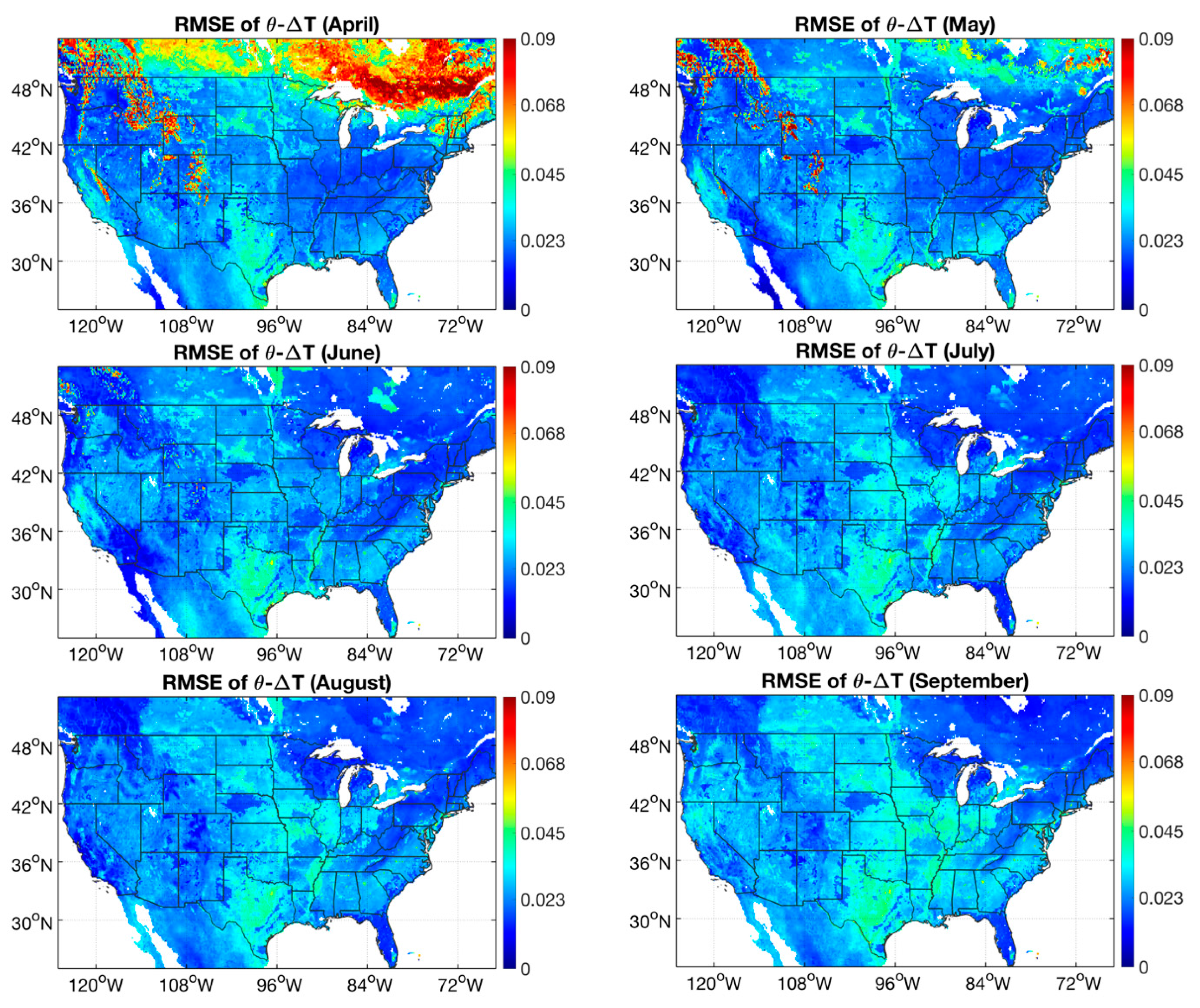
3. Evaluation of the Downscaling Algorithm

For examining performance of the downscaling algorithm at different regions and seasons, the R2 and RMSE (root mean squared error) between θ and corresponding Δ T s of descending overpass times using the NLDAS data between 1981 and 2016 by each month between April and September are mapped in Figure 2 and Figure 3. The other months from October to March were excluded for building the downscaling model, as the NLDAS SM had poor correlations with in situ observations in the northern CONUS region during cold months and was suggested not to be used, due to the biases caused by frozen soil water content [72]. In these maps, the R2 and RMSE are averaged from all the NDVI classes for each NLDAS grid. It is found that the western part of CONUS generally has higher R2 (basically > 0.2 in warm months) than the eastern CONUS. Some possible factors may have an impact on the accuracy of NLDAS variables SM and temperature estimations, such as vegetation type, vegetation structure, and soil texture. This can be referred to the related research on validating NLDAS SM using ground observations over the CONUS region, which found better validation statistical variables in the western region at shallow depth soil layer [72,73]. Low R2 values are also noted in the Rocky Mountain Region, where is usually covered by snow until mid-summer. The R2 shows an increasing trend from April to July for both the western/eastern regions and it reaches the peak in July. The southwestern states have overall strong R2 (0.6–0.8) associated with sparse vegetation coverage and low amounts of precipitation through the entire year. The R2 slowly decreases from July to September. The western part has greater changes of R2 than the eastern part through all six months. The above facts may also be determined by the data quality of NLDAS SM estimates: the research [72] found the seasonal variability of validation statistical variables for the NLDAS SM, of which the hottest months (July and August) tend to be more accurate than the other months. These could be explained by the influence of frozen water content in the soil layer or the slow response of the increase in SM in wet seasons (spring and fall).
The RMSE maps for SM prediction do not show clear regional distribution patterns, the only exception being a high RMSE in the north of U.S. and Rocky Mountain region in April–May, where could be covered by snow. Similarly, we do not observe clear seasonal trends of RMSE’s variation from cool to warm months. The RMSE values are mostly <0.03 m3/m3 throughout the entire CONUS region, except the aforementioned northern and mountainous regions with high RMSEs in cool months.
Figure 4 and Table 1 show four NLDAS grids of modeled θ Δ T s relationships of different NDVI classes in July between 1981 and 2016. These represent regions of different vegetation coverage and SM conditions. The locations include (1) Walnut Gulch, Arizona, (2) Stillwater, Oklahoma, (3) Reynolds Creek, Idaho, and (4) Ames, Iowa, all of which have permanent long-term SM monitoring stations. Overall, it can be summarized that θ and Δ T s are negatively correlated, and the fit lines for all NDVI classes have similar slope values. In general, θ Δ T s correlations have higher R2 for descending overpasses than ascending overpasses. This fact is also reflected on θ Δ T s scatterplots, where the descending overpass scatterplots are more concentrated. The R2 of descending θ Δ T s relationships range from 0.493 to 0.784 in Walnut Gulch—clearly higher than the other three locations. This is probably attributed to the Walnut Gulch having the overall narrowest NDVI range (0–0.4), so the θ Δ T s relationship is less complicated by vegetation. In contrast, Ames has the worst overall R2 (0.092–0.275) and has the widest NDVI range between 0–0.8. On another hand, R2 values do not show clear decreasing trends as NDVI class increases for all four locations for either descending/ascending overpasses. The outliers are noted for all NDVI classes from the scatterplots in Figure 4, indicating the impact of vegetation on θ Δ T s relationships. However, such impact does not strengthen when NDVI increases either. In addition, according to the sample numbers shown in Table 1, the NDVI classes with few points may contain more uncertainties with respect to the regression analysis, and the R2 may be relatively higher or lower than the other classes, such as NDVI class 0.3–0.4 for Walnut Gulch, 0–0.1 for Stillwater, and 0.4–0.5 for Reynolds Creek.

4. Downscaled AMSR2 Soil Moisture Results

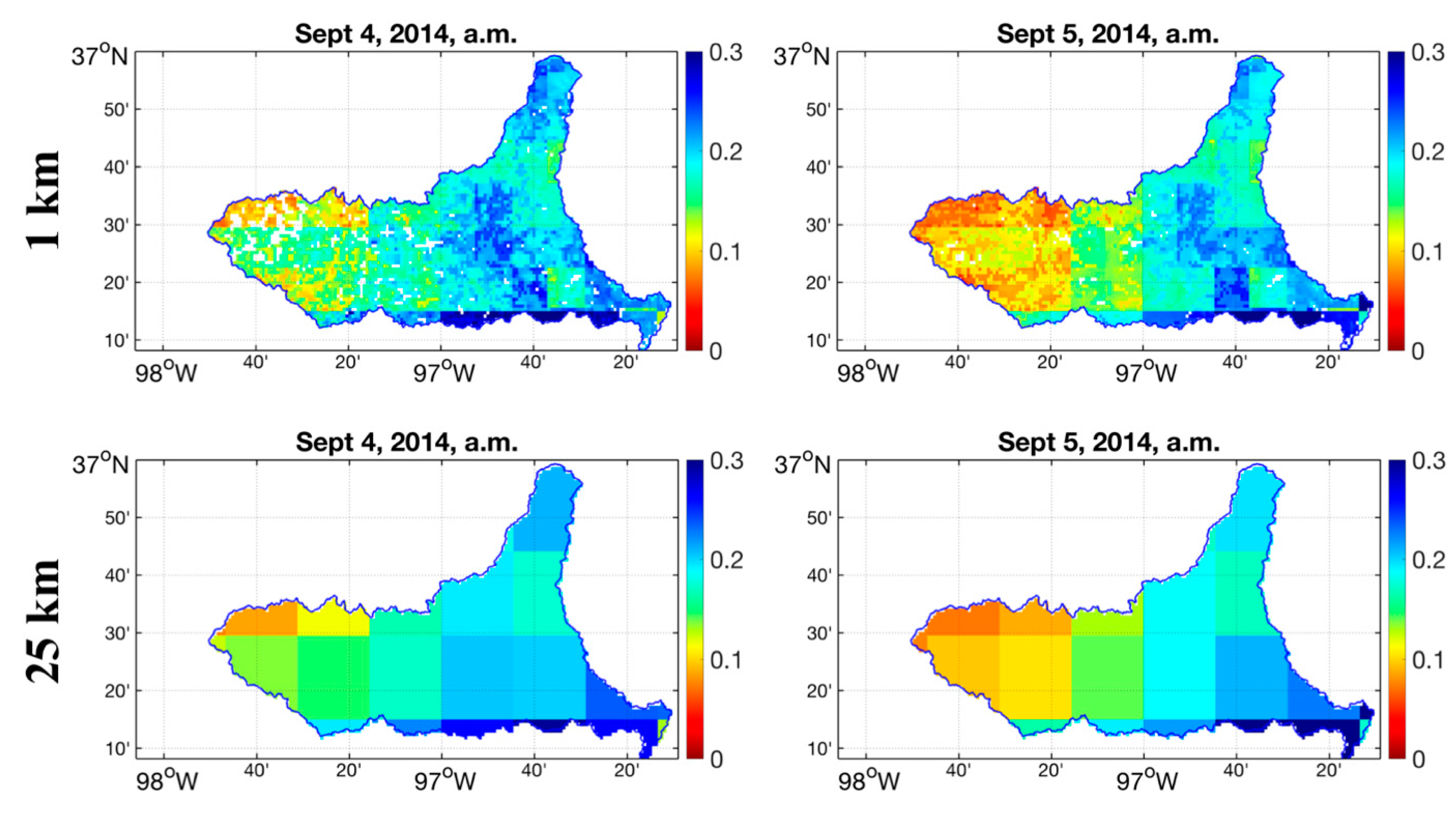
4.1. Interpretation of Soil Moisture Maps
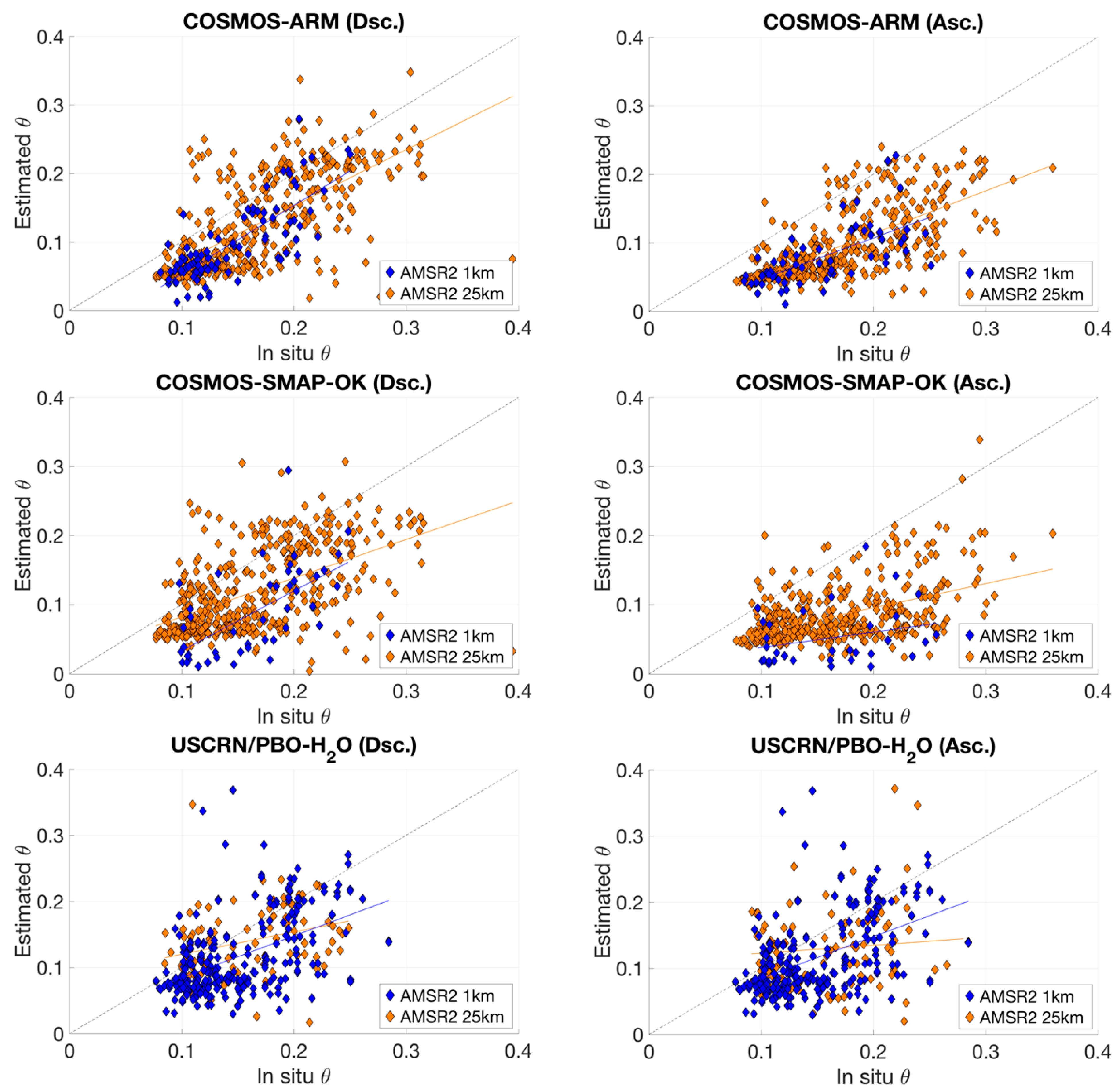
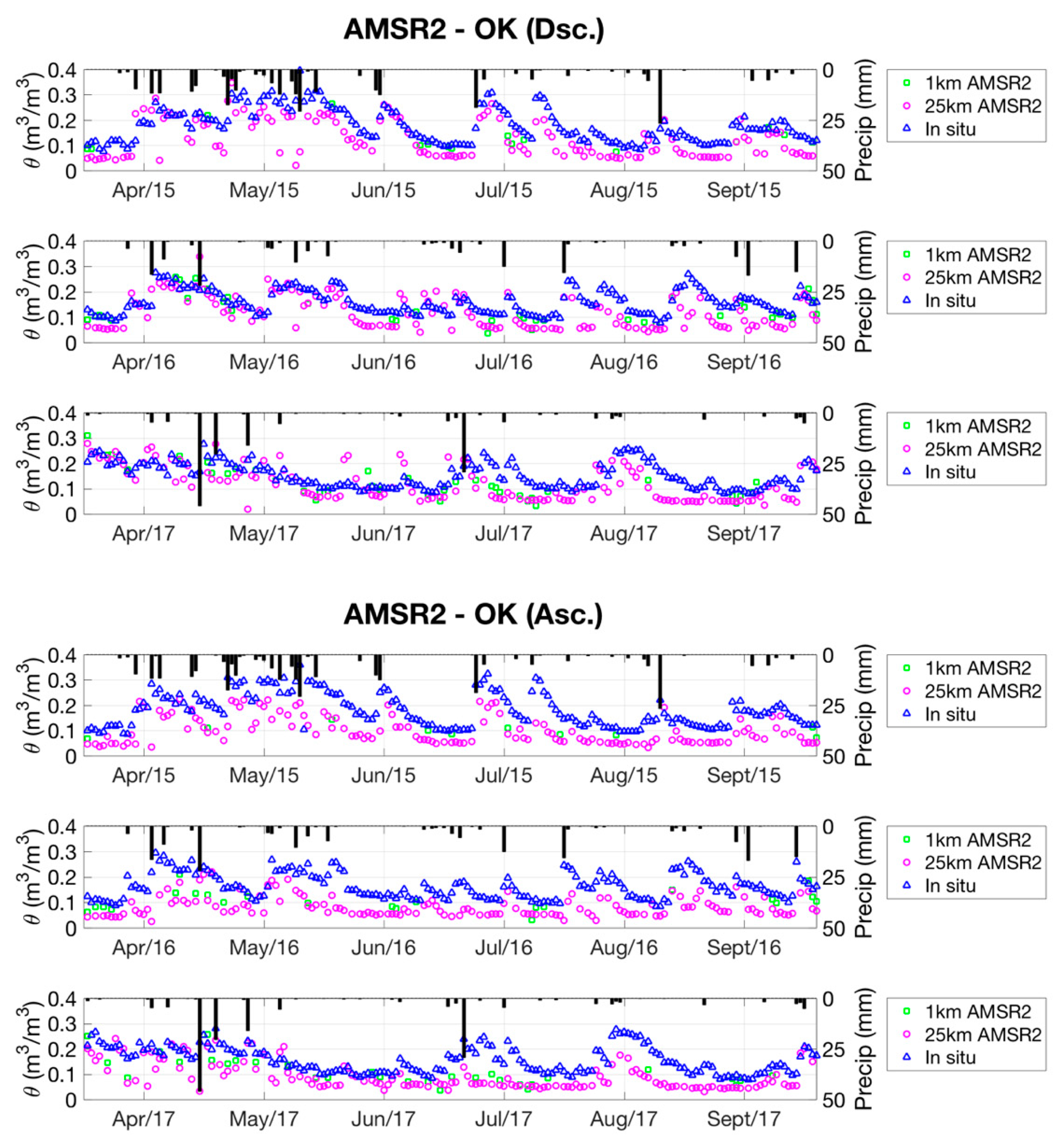
In Figure 5, the 1 km downscaled AMSR2 SM are mapped to compare with the original 25 km AMSR2 SM at the CONUS region scale as well as the watershed scale. The 1 km AMSR2 SM from June of morning overpasses (descending overpasses) have very similar spatial distribution patterns as the 25 km SM. However, they show spatial variabilities at a finer spatial scale, especially in the regions with heterogeneous SM conditions, such as the mid-west region in the Mississippi river basin.
When one focuses on the watershed scale, as Figure 6 shown the 1 km/25 km AMSR2 SM of morning overpasses in the Black Bear–Red Rock watershed, central Oklahoma from 4–5 September 2014, we can observe the different SM spatial distribution patterns in the west/east side of Arkansas River (The river path is shown in Figure 1) in 1 km SM maps, which are not observed in 25 km maps. The SM dry-down trends are also better captured in 1 km SM maps. The western bank of the Arkansas River demonstrates greater heterogeneity than the eastern bank. This is probably due to the land cover type: the eastern part of the watershed is dominated by grassland, while the agricultural land composes the western part. In addition, wetter regions in the center of the watershed can be noted, which are not captured in the 25 km SM maps. These regions are close to the Sooner Lake and a big bend of Arkansas River. Similarly, another good example in Western U.S. of Figure 7 shows contrast between 1 and 25 km SM of ascending overpasses in the San Pedro River watershed, Arizona, from 3–10 May 2016. The 25 km SM maps show nearly no spatial or temporal variation throughout the entire watershed during this period. In contrast to this, the downscaled 1 km SM clearly demonstrates several wetter regions along the west and east sides of the watershed boundaries, which are parts of the Coronado national forest. Besides this, we can also observe a wetter region across the middle of the watershed which corresponds to the river and alluvial plain. This feature agrees to the topography shown in Figure 1. Another issue about the performance of the downscaling algorithm is worth noticing: the downscaled 1 km SM maps show sharp edges in both Figure 6 and Figure 7.
Particularly, in Figure 6, the sharp-edge issue is more clearly observed once great difference between adjacent 25 km grids. And, the sharp edges exactly correspond to the spatial pattern of 25 km SM maps. In Figure 7, the shape edges are also found at the center of the watershed of the 1 km SM maps, while there is little spatial variability in the 25 km SM maps. The sharp-edge issue can be concluded for two reasons: Firstly, the downscaling algorithm corrects the 25 km resolution AMSR2 SM by using the 1 km SM estimates derived from MODIS LST within the 25 km grid boundaries. However, there is no smoothing step performed on adjacent 25 km grids. The second reason is the discontinuity of the spatial pattern in the 1 km estimated SM grids, which is mainly caused by adjacent 12.5 km NLDAS grids. The downscaling algorithm was built at the 12.5 km NLDAS scale, and adjacent NLDAS grids may have quite different θ Δ T s relationships.

4.2. Validation

The 1 km downscaled and 25 km AMSR2 SM were validated using ISMN in situ SM measurements in the Black Bear-Red Rock watershed, Oklahoma, between 2015 and 2017, as Figure 8 and Figure 9 shown. In this validation, the ISMN in situ measurements within each 1 km/25 km AMSR2 SM grid were averaged for validating. Please note that there are fewer data points for the 1 km than for the 25 km SM validations for all the stations, as the 1 km downscaled SM results usually have less coverage than 25 km due to the cloud contamination and satellite swath gap issues. From Figure 8, it can be seen that the slopes of 1 km SM validation results of descending overpasses are closer to 1 than the 25 km validation plots. The validation metrics improve from the original 25 km to the 1 km SM for descending overpasses, as shown in Table 2. The R2 of 1 km SM validations ranges from 0.284 to 0.608, which is much better than the overall range of 0.094–0.449 for 25 km SM. Improvement is also noted in the unbiased RMSE (ubRMSE), which ranges from 0.036 to 0.079 m3/m3 for the 1 km SM in comparison to the range of 0.036–0.052 m3/m3 for the 25 km SM. Considering the data accuracy of the JAXA algorithm retrieved AMSR2 SM, which has the overall ubRMSE of 0.059 m3/m3 validated by core validation sites [64], the performance of the downscaling algorithm in CONUS is fairly good and the overall bias is also improved. For the ascending overpasses, it can be seen that the R2 and ubRMSE are improved from 25 to 1 km, but degradation for bias is also noted. In addition to this, an overall underestimation trend is observed for the downscaled 1 km SM for both descending/ascending overpasses. From Figure 8 and the bias values of Table 2, it appears that the 1 km SM for the ascending overpasses are underestimated by a larger amount than for the descending overpasses. Additionally, for the 25 km SM validation, descending overpasses generally have better R2 and ubRMSE than ascending overpasses, but worse bias. By studying Figure 8, the reasons could be that the 25 km SM validation results for ascending are better correlated and the scatter points are more concentrated, but also show stronger dry-biased tendency. By studying the validation results between stations, we found that the COSMOS stations: COSMOS-ARM (Atmospheric Radiation Measurement) and COSMOS-SMAP-OK have improved overall R2 but worse overall ubRMSE compared with other stations. On the contrary, the stations of USCRN-Stillwater and PBO-H2O-OK have lower overall ubRMSE and the points on the scatterplots are closer to the 1-1 line, but worse R2. Referring to the previous research on validating in situ SM measurements, the COSMOS SM measurements are recorded by cosmic-ray probes from the wireless sensor network (SoilNET) and the overall accuracy is within 0.04 m3/m3 at heterogeneous farmland. Research also found that the vegetation water content, biomass, air pressure, and other factors may have an impact on the accuracy of COSMOS SM [74,75,76]. On the other hand, USCRN is with an average random error of ~0.012 m3/m3 by triple collocation validation method in the CONUS region, and the largest error was noted at shallower depths [77,78,79]. The USCRN provides more reliable SM measurements than COSMOS, so the downscaled results validated by USCRN show better agreements and smaller overall ubRMSE.
Figure 9 shows time series plots of daily averaged 1 km/25 km AMSR2 SM estimates along with ISMN in situ SM measurements, as well as the corresponding GPM daily precipitation at the COSMOS-SMAP-Oklahoma station between 2015 and 2017. It can be observed that both the 1 km/25 km AMSR SM estimates for the descending/ascending overpasses have similar dry-down and wetting trends when compared to the in situ measurements. In addition to this, the underestimation tendencies are observed for both 1 km and 25 km AMSR2 SM estimates, which correspond to the Figure 8 scatterplots. All three SM data sets show less discrepancy for the descending overpasses than ascending overpasses. Possible reasons for this behavior could be: (1) a remote sensing SM estimate represents the average SM value within the grid domain, while in situ measurements represent point locations, and (2) AMSR2 SM estimates of descending overpasses have better overall accuracy in the validation sites, due to the uniform surface temperature and soil profiles during night time [5,20]. In addition, the precipitation may have an impact on the accuracy of the estimated 1 km/25 km AMSR2 SM. The impact includes contamination on microwave signals, as well as the slow response of soil moisture retrievals to precipitation events [80]. In Figure 9, there are large discrepancies between the AMSR2 SM estimates and the in situ SM for ascending overpasses during rainy seasons, such as mid-April to mid-June of 2015 and mid-April to late-May of 2016.

5. Summary

A SM downscaling algorithm for use with passive microwave satellite estimates was modified, applied as well as validated using in situ ground measurements from an in situ SM database ISMN. The algorithm is based on vegetation modulated relationships between the surface layer SM for descending/ascending overpasses and the corresponding surface temperature difference. The modified algorithm was developed based on only three variables land surface temperature, SM, and NDVI. The use of other related land surface variables, such as precipitation and soil properties, was avoided in the current approach. The algorithm was evaluated in the CONUS region for the months between April and September, and was found generally performed better over the western US than eastern US. The algorithm also demonstrated seasonal variability of performance and the hottest months, July and August, have stronger θ Δ T s correlations than the other months. The modeled relationships were applied to 1 km MODIS Aqua LST data to downscale coarse resolution 25 km AMSR2 microwave radiometer SM retrieved using the JAXA algorithm. The AMSR2 SM data for the CONUS region between 2013 and 2017 were implemented for producing the 1 km downscaled SM products. SM spatial variability as well as dry-down and wetting trends for selected watersheds in Arizona and Oklahoma were found to be better characterized by the downscaled SM than the coarse SM product. The downscaled SM product was validated using ISMN in situ SM observations in Oklahoma and the assessment results show better overall consistency for the downscaled SM product as compared to the coarser resolution 25 km AMSE2 SM estimates (R2 increased by 0.141 for descending overpass and increased by 0.215 for ascending overpass). For the downscaled AMSR2 SM, the overall R2 shows a good correlation with the in situ SM. The precipitation events had an impact on the performance of SM downscaling algorithm due to the reduction in the sensing depth of the microwave signals [11]. The underestimation is noted for both the 1 km downscaled and 25 km AMSR2 SM estimates when compared with in situ data.
In interpreting the validation reported here, there are several issues concerning remotely sensed SM and in situ observations that should be considered [81,82]. First, the passive microwave remotely sensed data originate from an ellipsoidal region at a scale of tens of kilometers, as opposed to the ground observations that record the SM at the point scale. Second, there are potential mismatches in the sensing depths among all the SM data sets. The brightness temperatures sensed by passive microwave sensors (AMSR2) and MODIS, SM outputs from NLDAS, and the in situ SM measured by ground stations are all at different depths. A previous study found that satellite-based SM is noisier than land surface model data [83]. Furthermore, the passive microwave sensors can penetrate a few centimeters, while the MODIS penetrates only a few millimeters, which are compared with the NLDAS SM outputs at a 0–10 cm depth and the ground measurements at a 5 cm depth.

Author Contributions

V.L. coordinated this study and designed the original algorithms for the downscaling of the soil moisture for AMSR-E. B.F. modified the algorithm for AMSR2 and carried out the implementation. R.B. advised the team on the proper implementation of the algorithm and on the validation. T.J.J. was responsible for the validation and the data quality control.

Funding

The work was funded by the NASA Terrestrial Hydrology Program (Program Manager: Jared Entin) and the NASA's Western Water Applications Office (WWAO) Program (Program Manager: Bradley Doorn).

Conflicts of Interest

The authors declare no conflict of interest.

References

  1. Njoku, E.G.; Entekhabi, D. Passive microwave remote sensing of soil moisture. J. Hydrol. 1996, 184, 101–129. [Google Scholar] [CrossRef] [Green Version]
  2. Jackson, T.J.; Schmugge, T.J. Passive microwave remote sensing system for soil moisture: Some supporting research. IEEE Trans. Geosci. Remote Sens. 1989, 27, 225–235. [Google Scholar] [CrossRef]
  3. Schmugge, T.; Jackson, T.J. Mapping surface soil moisture with microwave radiometers. Meteorol. Atmos. Phys. 1994, 54, 213–223. [Google Scholar] [CrossRef]
  4. Jackson, T.J.; Le Vine, D.M.; Hsu, A.Y.; Oldak, A.; Starks, P.J.; Swift, C.T.; Isham, J.D.; Haken, M. Soil moisture mapping at regional scales using microwave radiometry: The Southern Great Plains Hydrology Experiment. IEEE Trans. Geosci. Remote Sens. 1999, 37, 2136–2151. [Google Scholar] [CrossRef]
  5. Jackson, T.J.; Cosh, M.H.; Bindlish, R.; Starks, P.J.; Bosch, D.D.; Seyfried, M.; Goodrich, D.C.; Moran, M.S.; Du, J. Validation of advanced microwave scanning radiometer soil moisture products. IEEE Trans. Geosci. Remote Sens. 2010, 48, 4256–4272. [Google Scholar] [CrossRef]
  6. Lakshmi, V.; Susskind, J. Comparison of TOVS—Derived land surface variables with ground observations. J. Geophys. Res. Atmos. 2000, 105, 2179–2190. [Google Scholar] [CrossRef]
  7. Lakshmi, V. The role of satellite remote sensing in the prediction of ungauged basins. Hydrol. Proc. 2004, 18, 1029–1034. [Google Scholar] [CrossRef]
  8. Lakshmi, V. Remote sensing of soil moisture. ISRN Soil Sci. 2013, 2013. [Google Scholar] [CrossRef]
  9. Njoku, E.G.; Jackson, T.J.; Lakshmi, V.; Chan, T.K.; Nghiem, S.V. Soil moisture retrieval from AMSR–E. IEEE Trans. Geosci. Remote Sens. 2003, 41, 215–229. [Google Scholar] [CrossRef]
  10. Chan, S.K.; Bindlish, R.; O’Neill, P.E.; Njoku, E.; Jackson, T.; Colliander, A.; Chen, F.; Burgin, M.; Dunbar, S.; Piepmeier, J.; et al. Assessment of the SMAP passive soil moisture product. IEEE Trans. Geosci. Remote Sens. 2016, 54, 4994–5007. [Google Scholar] [CrossRef]
  11. Jackson, T.J.; Bindlish, R.; Cosh, M.H.; Zhao, T.; Starks, P.J.; Bosch, D.D.; Seyfried, M.; Moran, M.S.; Goodrich, D.C.; Kerr, Y.H.; et al. Validation of Soil Moisture and Ocean Salinity (SMOS) soil moisture over watershed networks in the US. IEEE Trans. Geosci. Remote Sens. 2012, 50, 1530–1543. [Google Scholar] [CrossRef] [Green Version]
  12. Bindlish, R.; Jackson, T.; Cosh, M.; Zhao, T.; O’neill, P. Global soil moisture from the Aquarius/SAC–D satellite: Description and initial assessment. IEEE Geosci. Remote Sens. Lett. 2015, 12, 923–927. [Google Scholar] [CrossRef]
  13. Bindlish, R.; Barros, A.P. Subpixel variability of remotely sensed soil moisture: An inter–comparison study of SAR and ESTAR. IEEE Trans. Geosci. Remote Sens. 2002, 40, 326–337. [Google Scholar] [CrossRef]
  14. Mladenova, I.; Lakshmi, V.; Walker, J.P.; Panciera, R.; Wagner, W.; Doubkova, M. Validation of the ASAR global monitoring mode soil moisture product using the NAFE’05 data set. IEEE Trans. Geosci. Remote Sens. 2010, 48, 2498–2508. [Google Scholar] [CrossRef]
  15. Minet, J.; Bogaert, P.; Vanclooster, M.; Lambot, S. Validation of ground penetrating radar full–waveform inversion for field scale soil moisture mapping. J. Hydrol. 2012, 424, 112–123. [Google Scholar] [CrossRef]
  16. Sridhar, V.; Jaksa, W.T.A.; Fang, B.; Lakshmi, V.; Hubbard, K.G.; Jin, X. Evaluating bias–corrected AMSR–E soil moisture using in situ observations and model estimates. Vadose Zone J. 2013, 12. [Google Scholar] [CrossRef]
  17. Imaoka, K.; Kachi, M.; Fujii, H.; Murakami, H.; Hori, M.; Ono, A.; Igarashi, T.; Nakagawa, K.; Oki, T.; Honda, Y.; et al. Global Change Observation Mission (GCOM) for monitoring carbon, water cycles, and climate change. Proc. IEEE 2010, 98, 717–734. [Google Scholar] [CrossRef]
  18. Oki, T.; Imaoka, K.; Imaoka, M. AMSR instruments on GCOM–W1/2: Concepts and applications. In Proceedings of the 2010 IEEE International Geoscience and Remote Sensing Symposium (IGARSS), Honolulu, HI, USA, 25–30 July 2010. [Google Scholar]
  19. Maeda, T.; Taniguchi, Y.; Imaoka, K. GCOM-W1 AMSR2 level 1R product: Dataset of brightness temperature modified using the antenna pattern matching technique. IEEE Trans. Geosci. Remote Sens. 2016, 2, 770–782. [Google Scholar] [CrossRef]
  20. Cho, E.; Moon, H.; Choi, M. First assessment of the Advanced Microwave Scanning Radiometer 2 (AMSR2) soil moisture contents in Northeast Asia. J. Meteorol. Soc. Jpn. Ser. II 2015, 93, 117–129. [Google Scholar] [CrossRef]
  21. Bindlish, R.; Cosh, M.H.; Jackson, T.J.; Koike, T.; Fujii, H.; Chan, S.K.; Asanuma, J.; Berg, A.; Bosch, D.D.; Caldwell, T.; et al. GCOM–W AMSR2 soil moisture product validation using core validation sites. IEEE J. Sel. Top. Appl. Earth Obs. Remote Sens. 2018, 11, 209–219. [Google Scholar] [CrossRef]
  22. Koike, T. Soil Moisture Algorithm Descriptions of GCOM–W1 AMSR2 (Rev. A); Earth Observation Research Center, Japan Aerospace Exploration Agency: Ibaraki, Japan, 2013. [Google Scholar]
  23. Jackson, T.J., III. Measuring surface soil moisture using passive microwave remote sensing. Hydrol. Proc. 1993, 7, 139–152. [Google Scholar] [CrossRef]
  24. Owe, M.; de Jeu, R.A.; Walker, J. A methodology for surface soil moisture and vegetation optical depth retrieval using the microwave polarization difference index. IEEE Trans. Geosci. Remote Sens. 2001, 39, 1643–1654. [Google Scholar] [CrossRef] [Green Version]
  25. Lakshmi, V.; Czajkowski, K.; Dubayah, R.; Susskind, J. Land surface air temperature mapping using TOVS and AVHRR. Int. J. Remote Sens. 2001, 22, 643–662. [Google Scholar] [CrossRef]
  26. Bolten, J.D.; Lakshmi, V.; Njoku, E.G. Soil moisture retrieval using the passive/active L–and S–band radar/radiometer. IEEE Trans. Geosci. Remote Sens. 2003, 41, 2792–2801. [Google Scholar] [CrossRef]
  27. Narayan, U.; Lakshmi, V.; Njoku, E.G. Retrieval of soil moisture from passive and active L/S band sensor (PALS) observations during the Soil Moisture Experiment in 2002 (SMEX02). Remote Sens. Environ. 2004, 92, 483–496. [Google Scholar] [CrossRef]
  28. Piles, M.; Entekhabi, D.; Camps, A. A change detection algorithm for retrieving high–resolution soil moisture from SMAP radar and radiometer observations. IEEE Trans. Geosci. Remote Sens. 2009, 47, 4125–4131. [Google Scholar] [CrossRef]
  29. Narayan, U.; Lakshmi, V.; Jackson, T.J. High–resolution change estimation of soil moisture using L–band radiometer and radar observations made during the SMEX02 experiments. IEEE Trans. Geosci. Remote Sens. 2006, 44, 1545–1554. [Google Scholar] [CrossRef]
  30. Narayan, U.; Lakshmi, V. Characterizing subpixel variability of low resolution radiometer derived soil moisture using high resolution radar data. Water Resour. Res. 2008, 44. [Google Scholar] [CrossRef] [Green Version]
  31. Peng, J.; Loew, A.; Merlin, O.; Verhoest, N.E. A review of spatial downscaling of satellite remotely sensed soil moisture. Rev. Geophys. 2017, 55, 341–366. [Google Scholar] [CrossRef] [Green Version]
  32. Parada, L.M.; Liang, X. Optimal multiscale Kalman filter for assimilation of near-surface soil moisture into land surface models. J. Geophys. Res. Atmos. 2004, 109. [Google Scholar] [CrossRef] [Green Version]
  33. Pan, M.; Wood, E.F.; McLaughlin, D.B.; Entekhabi, D.; Luo, L. A multiscale ensemble filtering system for hydrologic data assimilation. Part I: Implementation and synthetic experiment. J. Hydrometeorol. 2009, 10, 794–806. [Google Scholar] [CrossRef]
  34. Sahoo, A.K.; De Lannoy, G.J.; Reichle, R.H.; Houser, P.R. Assimilation and downscaling of satellite observed soil moisture over the Little River Experimental Watershed in Georgia, USA. Adv. Water Resour. 2013, 52, 19–33. [Google Scholar] [CrossRef] [Green Version]
  35. Mallick, K.; Bhattacharya, B.K.; Patel, N.K. Estimating volumetric surface moisture content for cropped soils using a soil wetness index based on surface temperature and NDVI. Agric. For. Meteorol. 2009, 149, 1327–1342. [Google Scholar] [CrossRef]
  36. Ranney, K.J.; Niemann, J.D.; Lehman, B.M.; Green, T.R.; Jones, A.S. A method to downscale soil moisture to fine resolutions using topographic, vegetation, and soil data. Adv. Water Resour. 2015, 76, 81–96. [Google Scholar] [CrossRef] [Green Version]
  37. Merlin, O.; Al Bitar, A.; Walker, J.P.; Kerr, Y. An improved algorithm for disaggregating microwave–derived soil moisture based on red, near–infrared and thermal–infrared data. Remote Sens. Environ. 2010, 114, 2305–2316. [Google Scholar] [CrossRef] [Green Version]
  38. Merlin, O.; Escorihuela, M.J.; Mayoral, M.A.; Hagolle, O.; Al Bitar, A.; Kerr, Y. Self–calibrated evaporation–based disaggregation of SMOS soil moisture: An evaluation study at 3km and 100m resolution in Catalunya, Spain. Remote Sens. Environ. 2013, 130, 25–38. [Google Scholar] [CrossRef] [Green Version]
  39. Merlin, O.; Malbéteau, Y.; Notfi, Y.; Bacon, S.; Khabba, S.E.R.S.; Jarlan, L. Performance metrics for soil moisture downscaling methods: Application to DISPATCH data in central Morocco. Remote Sens. 2015, 7, 3783–3807. [Google Scholar] [CrossRef]
  40. Merlin, O.; Chehbouni, A.; Walker, J.P.; Panciera, R.; Kerr, Y.H. A simple method to disaggregate passive microwave–based soil moisture. IEEE Trans. Geosci. Remote Sens. 2008, 46, 786–796. [Google Scholar] [CrossRef] [Green Version]
  41. Fang, B.; Lakshmi, V. AMSR–E Soil Moisture Disaggregation Using MODIS and NLDAS Data. Remote Sens. Terr. Water Cycle 2014, 206, 277. [Google Scholar]
  42. Piles, M.; Camps, A.; Vall–Llossera, M.; Corbella, I.; Panciera, R.; Rudiger, C.; Kerr, Y.H.; Walker, J. Downscaling SMOS–derived soil moisture using MODIS visible/infrared data. IEEE Trans. Geosci. Remote Sens. 2011, 49, 3156–3166. [Google Scholar] [CrossRef]
  43. Peng, J.; Loew, A.; Zhang, S.; Wang, J.; Niesel, J. Spatial downscaling of satellite soil moisture data using a vegetation temperature condition index. IEEE Trans. Geosci. Remote Sens. 2016, 54, 558–566. [Google Scholar] [CrossRef]
  44. Choi, M.; Hur, Y. A microwave–optical/infrared disaggregation for improving spatial representation of soil moisture using AMSR–E and MODIS products. Remote Sens. Environ. 2012, 124, 259–269. [Google Scholar] [CrossRef]
  45. Sánchez–Ruiz, S.; Piles, M.; Sánchez, N.; Martínez–Fernández, J.; Vall–llossera, M.; Camps, A. Combining SMOS with visible and near/shortwave/thermal infrared satellite data for high resolution soil moisture estimates. J. Hydrol. 2014, 516, 273–283. [Google Scholar] [CrossRef]
  46. Fang, B.; Lakshmi, V.; Bindlish, R.; Jackson, T.J.; Cosh, M.; Basara, J. Passive microwave soil moisture downscaling using vegetation index and skin surface temperature. Vadose Zone J. 2013, 12, 273–283. [Google Scholar] [CrossRef]
  47. Fang, B.; Lakshmi, V. Soil Moisture at Watershed Scale: Remote Sensing Techniques. J. Hydrol. 2014, 516, 258–272. [Google Scholar] [CrossRef]
  48. Fang, B.; Lakshmi, V.; Bindlish, R.; Jackson, T.J. Downscaling of SMAP soil moisture using land surface temperature and vegetation data. Vadose Zone J. 2018. accepted. [Google Scholar] [CrossRef]
  49. Fujii, H.; Koike, T.; Imaoka, K. Improvement of the AMSR–E algorithm for soil moisture estimation by introducing a fractional vegetation coverage dataset derived from MODIS data. J. Remote Sens. Soc. Jpn. 2009, 29, 282–292. [Google Scholar]
  50. Imaoka, K.; Kachi, M.; Kasahara, M.; Ito, N.; Nakagawa, K.; Oki, T. Instrument performance and calibration of AMSR-E and AMSR2. Int. Arch. Photogram. Remote Sens. Spat. Inf. Sci. 2010, 8, 13–18. [Google Scholar]
  51. Minacapilli, M.; Iovino, M.; Blanda, F. High resolution remote estimation of soil surface water content by a thermal inertia approach. J. Hydrol. 2009, 379, 229–238. [Google Scholar] [CrossRef]
  52. Zhao, W.; Li, A. A Downscaling Method for Improving the Spatial Resolution of AMSR–E Derived Soil Moisture Product Based on MSG–SEVIRI Data. Remote Sens. 2013, 5, 6790–6811. [Google Scholar] [CrossRef]
  53. Cosgrove, B.A.; Lohmann, D.; Mitchell, K.E.; Houser, P.R.; Wood, E.F.; Schaake, J.C.; Robock, A.; Marshall, C.; Sheffield, J.; Duan, Q.; et al. Real-time and retrospective forcing in the North American Land Data Assimilation System (NLDAS) project. J. Geophys. Res. Atmos. 2013, 108. [Google Scholar] [CrossRef]
  54. Mitchell, K.E.; Lohmann, D.; Houser, P.R.; Wood, E.F.; Schaake, J.C.; Robock, A.; Cosgrove, B.A.; Sheffield, J.; Duan, Q.; Luo, L.; et al. The multi-institution North American Land Data Assimilation System (NLDAS): Utilizing multiple GCIP products and partners in a continental distributed hydrological modeling system. J. Geophys. Res. Atmos. 2004, 109. [Google Scholar] [CrossRef] [Green Version]
  55. Robock, A.; Luo, L.; Wood, E.F.; Wen, F.; Mitchell, K.E.; Houser, P.R.; Schaake, J.C.; Lohmann, D.; Cosgrove, B.; Sheffield, J.; et al. Evaluation of the North American Land Data Assimilation System over the southern Great Plains during the warm season. J. Geophys. Res. Atmos. 2003, 108. [Google Scholar] [CrossRef] [Green Version]
  56. Schaake, J.C.; Duan, Q.; Koren, V.; Mitchell, K.E.; Houser, P.R.; Wood, E.F.; Robock, A.; Lettenmaier, D.P.; Lohmann, D.; Cosgrove, B.; et al. An intercomparison of soil moisture fields in the North American Land Data Assimilation System (NLDAS). J. Geophys. Res. Atmos. 2004, 109. [Google Scholar] [CrossRef] [Green Version]
  57. Wan, Z.; Li, Z.L. A physics–based algorithm for retrieving land–surface emissivity and temperature from EOS/MODIS data. IEEE Trans. Geosci. Remote Sens. 1997, 35, 980–996. [Google Scholar]
  58. Tucker, C.J. Red and photographic infrared linear combinations for monitoring vegetation. Remote Sens. Environ. 1979, 8, 127–150. [Google Scholar] [CrossRef] [Green Version]
  59. Dorigo, W.A.; Xaver, A.; Vreugdenhil, M.; Gruber, A.; Hegyiova, A.; Sanchis–Dufau, A.D.; Zamojski, D.; Cordes, C.; Wagner, W.; Drusch, M. Global automated quality control of in situ soil moisture data from the International Soil Moisture Network. Vadose Zone J. 2013, 12. [Google Scholar] [CrossRef]
  60. Gruber, A.; Dorigo, W.A.; Zwieback, S.; Xaver, A.; Wagner, W. Characterizing coarse–scale representativeness of in situ soil moisture measurements from the International Soil Moisture Network. Vadose Zone J. 2013, 12. [Google Scholar] [CrossRef]
  61. Larson, K.M.; Small, E.E.; Gutmann, E.D.; Bilich, A.L.; Braun, J.J.; Zavorotny, V.U. Use of GPS receivers as a soil moisture network for water cycle studies. Geophys. Res. Lett. 2008, 35. [Google Scholar] [CrossRef] [Green Version]
  62. Herring, T.A.; Melbourne, T.I.; Murray, M.H.; Floyd, M.A.; Szeliga, W.M.; King, R.W.; Phillips, D.A.; Puskas, C.M.; Santillan, M.; Wang, L. Plate Boundary Observatory and related networks: GPS data analysis methods and geodetic products. Rev. Geophys. 2016, 54, 759–808. [Google Scholar] [CrossRef] [Green Version]
  63. Schmugge, T.; Gloersen, P.; Wilheit, T.; Geiger, F. Remote sensing of soil moisture with microwave radiometers. J. Geophys. Res. 1974, 79, 317–323. [Google Scholar] [CrossRef] [Green Version]
  64. Choudhury, B.J.; Schmugge, T.J.; Chang, A.; Newton, R.W. Effect of surface roughness on the microwave emission from soils. J. Geophys. Res. Ocean. 1979, 84, 5699–5706. [Google Scholar] [CrossRef]
  65. Carlson, T.N.; Gillies, R.R.; Schmugge, T.J. An interpretation of methodologies for indirect measurement of soil water content. Agric. For. Meteorol. 1995, 77, 191–205. [Google Scholar] [CrossRef]
  66. Gillies, R.R.; Kustas, W.P.; Humes, K.S. A verification of the’triangle’method for obtaining surface soil water content and energy fluxes from remote measurements of the Normalized Difference Vegetation Index (NDVI) and surface e. Int. J. Remote Sens. 1997, 18, 3145–3166. [Google Scholar] [CrossRef]
  67. Hong, S.; Lakshmi, V.; Small, E.E.; Chen, F.; Tewari, M.; Manning, K.W. Effects of vegetation and soil moisture on the simulated land surface processes from the coupled WRF/Noah model. J. Geophys. Res. Atmos. 2009, 114. [Google Scholar] [CrossRef] [Green Version]
  68. Lakshmi, V.; Hong, S.; Small, E.E.; Chen, F. The influence of the land surface on hydrometeorology and ecology: New advances from modeling and satellite remote sensing. Hydrol. Res. 2011, 42, 95–112. [Google Scholar] [CrossRef]
  69. Pablos, M.; Piles, M.; Sánchez, N.; Vall–llossera, M.; Martínez–Fernández, J.; Camps, A. Impact of day/night time land surface temperature in soil moisture disaggregation algorithms. Eur. J. Remote Sens. 2016, 49. [Google Scholar] [CrossRef]
  70. Owe, M.; Van de Griend, A.A. Comparison of soil moisture penetration depths for several bare soils at two microwave frequencies and implications for remote sensing. Water Resour. Res. 1998, 34, 2319–2327. [Google Scholar] [CrossRef] [Green Version]
  71. Justice, C.O.; Vermote, E.; Townshend, J.R.; Defries, R.; Roy, D.P.; Hall, D.K.; Salomonson, V.V.; Privette, J.L.; Riggs, G.; Strahler, A. The Moderate Resolution Imaging Spectroradiometer (MODIS): Land remote sensing for global change research. IEEE Trans. Geosci. Remote Sens. 1998, 36, 1228–1249. [Google Scholar] [CrossRef]
  72. Xia, Y.; Ek, M.B.; Wu, Y.; Ford, T.; Quiring, S.M. Comparison of NLDAS–2 simulated and NASMD observed daily soil moisture. Part I: Comparison and analysis. J. Hydrometeorol. 2015, 16, 1962–1980. [Google Scholar] [CrossRef]
  73. Luo, L.; Robock, A.; Mitchell, K.E.; Houser, P.R.; Wood, E.F.; Schaake, J.C.; Lohmann, D.; Cosgrove, B.; Wen, F.; Sheffield, J.; et al. Validation of the North American land data assimilation system (NLDAS) retrospective forcing over the southern Great Plains. J. Geophys. Res. Atmos. 2003, 108. [Google Scholar] [CrossRef]
  74. Han, X.; Jin, R.; Li, X.; Wang, S. Soil moisture estimation using cosmic–ray soil moisture sensing at heterogeneous farmland. IEEE Geosci. Remote Sens. Lett. 2014, 11, 1659–1663. [Google Scholar]
  75. Rosolem, R.; Shuttleworth, W.J.; Zreda, M.; Franz, T.E.; Zeng, X.; Kurc, S.A. The effect of atmospheric water vapor on neutron count in the cosmic–ray soil moisture observing system. J. Hydrometeorol. 2013, 14, 1659–1671. [Google Scholar] [CrossRef]
  76. Zreda, M.; Shuttleworth, W.J.; Zeng, X.; Zweck, C.; Desilets, D.; Franz, T.; Rosolem, R. COSMOS: The cosmic–ray soil moisture observing system. Hydrol. Earth Syst. Sci. 2012, 16, 4079–4099. [Google Scholar] [CrossRef] [Green Version]
  77. Coopersmith, E.J.; Cosh, M.H.; Bell, J.E.; Crow, W.T. Multi–profile analysis of soil moisture within the US Climate Reference Network. Vadose Zone J. 2016, 15. [Google Scholar] [CrossRef]
  78. Bell, J.E.; Palecki, M.A.; Baker, C.B.; Collins, W.G.; Lawrimore, J.H.; Leeper, R.D.; Hall, M.E.; Kochendorfer, J.; Meyers, T.P.; Wilson, T.; et al. US Climate Reference Network soil moisture and temperature observations. J. Hydrometeorol. 2013, 14, 977–988. [Google Scholar] [CrossRef]
  79. Diamond, H.J.; Karl, T.R.; Palecki, M.A.; Baker, C.B.; Bell, J.E.; Leeper, R.D.; Easterling, D.R.; Lawrimore, J.H.; Meyers, T.P.; Helfert, M.R.; et al. US Climate Reference Network after one decade of operations: Status and assessment. Bull. Am. Meteorol. Soc. 2013, 94, 485–498. [Google Scholar] [CrossRef]
  80. Jin, K.-W.; Njoku, E.; Chan, S. Impact of Rainfall on the Retrieval of Soil Moisture using AMSR–E data. In Proceedings of the 2006 IEEE International Symposium on Geoscience and Remote Sensing, Denver, CO, USA, 31 July–4 August 2006. [Google Scholar]
  81. Zhang, X.; Zhang, T.; Zhou, P.; Shao, Y.; Gao, S. Validation analysis of SMAP and AMSR2 soil moisture products over the United States using ground–based measurements. Remote Sens. 2017, 9, 104. [Google Scholar] [CrossRef]
  82. Cosh, M.H.; Jackson, T.J.; Bindlish, R.; Prueger, J.H. Watershed scale temporal and spatial stability of soil moisture and its role in validating satellite estimates. Remote Sens. Environ. 2004, 92, 427–435. [Google Scholar] [CrossRef]
  83. Fang, L.; Hain, C.R.; Zhan, X.; Anderson, M.C. An inter–comparison of soil moisture data products from satellite remote sensing and a land surface model. Int. J. Appl. Earth Obs. Geoinf. 2016, 48, 37–50. [Google Scholar] [CrossRef]
Figure 1. The CONUS region and the sites for mapping and validating the SM downscaling algorithm: Black Bear–Red Watershed/Lower Cimarron Watershed, Oklahoma, and San Pedro River Watershed, Arizona. The ISMN SM monitoring ground stations are denoted in red.
Remotesensing 10 01575 g001
Figure 2. R2 maps in the CONUS region of AMSR2 descending overpasses from April to September at NLDAS grid spatial resolution 12.5 km. The R2 for each grid is computed from averaged R2 values between NLDAS SM and surface skin temperature corresponding to AMSR2 descending overpass times of all NDVI 0–1 classes.
Remotesensing 10 01575 g002
Figure 3. RMSE of SM estimation from the downscaling algorithm (m3/m3) maps in the CONUS region of AMSR2 descending overpasses from April to September at NLDAS grid spatial resolution 12.5 km. The RMSE for each grid is computed from averaged RMSE values between NLDAS SM and surface skin temperature corresponding to AMSR2 descending overpass times of all NDVI 0–1 classes.
Remotesensing 10 01575 g003
Figure 4. Scatterplots showing the relationships between NLDAS SM and surface skin temperature corresponding to different NDVI classes of descending/ascending overpasses from four selected NLDAS grids, which represents the regions of different vegetation coverage and SM condition: (1) Walnut Gulch, Arizona; (2) Stillwater, Oklahoma; (3) Reynolds Creek, Idaho; (4) Ames, Iowa.
Remotesensing 10 01575 g004
Figure 5. 1 km downscaled and 25 km AMSR2 L3 SM of descending overpasses (morning) in the CONUS region from three days in June 2015–2017.
Remotesensing 10 01575 g005
Figure 6. 1 km downscaled AMSR2 L3 SM compared with 25 km original SM estimates of descending overpasses (morning) showing spatial and temporal SM variabilities at the Black Bear–Red Rock watershed, central Oklahoma from 4–5 September 2014.
Remotesensing 10 01575 g006
Figure 7. 1 km downscaled AMSR2 L3 SM compared with 25 km original SM estimates of ascending overpasses (afternoon) showing spatial and temporal variabilities at San Pedro river watershed, southeastern Arizona from 4 days of early May 2016.
Remotesensing 10 01575 g007
Figure 8. Scatterplots of 1 km/25 km AMSR2 L3 SM of descending (Dsc.)/ascending (Asc.) overpasses between 2015 and 2017, validated using ISMN in situ data from the SM stations near Stillwater, Oklahoma, which are located in the lower Cimarron watershed.
Remotesensing 10 01575 g008
Figure 9. Time-series of daily averaged 1 km/25 km AMSR2 SM estimates of descending/ascending overpasses between 2015 and 2017 along with in situ measurements of corresponding times from the COSMOS station in Oklahoma for SMAP validation. The black bars are daily precipitation derived from a 10 km resolution GPM-IMERG L3 precipitation data.
Remotesensing 10 01575 g009
Table 1. R2 and sample numbers between NLDAS surface skin temperature and SM of descending/ascending overpasses in July from four selected NLDAS grids representing different vegetation and SM conditions in the CONUS region, including Walnut Gulch, Arizona; Stillwater, Oklahoma; Reynolds Creek, Idaho; Ames, Iowa.
Descending Overpasses
NDVIWalnut GulchStillwaterReynolds CreekAmes
0–0.10.6050.3410.3490.227
0.1–0.20.6910.4450.320.195
0.2–0.30.7840.4480.4040.154
0.3–0.40.4930.3760.3670.172
0.4–0.5-0.4930.4360.142
0.5–0.6-0.374-0.093
0.6–0.7-0.338-0.275
Ascending Overpasses
0–0.10.5750.2710.2320.07
0.1–0.20.6650.2240.1890.09
0.2–0.30.7790.0750.3230.342
0.3–0.40.2950.4830.2470.148
0.4–0.5-0.4930.1110.237
0.5–0.6-0.378-0.16
0.6–0.7-0.428-0.357
Sample Numbers
0–0.126980120118
0.1–0.259487221101
0.2–0.321810042294
0.3–0.413166291106
0.4–0.5-25543131
0.5–0.6-348-160
0.6–0.7-45-227
Table 2. Statistical variables of 1 km downscaled and 25 km AMSR2 SM of descending/ascending overpasses between 2015 and 2017, validated using ISMN in situ measurements which are located in the Black Bear–Red Rock watershed, Oklahoma.
Station1 km AMSR2 (Dsc.)1 km AMSR2 (Asc.)
R2ubRMSEBiasNumberR2ubRMSEBiasNumber
COSMOS-ARM0.6080.0480.048920.7540.0560.05645
COSMOS-SMAP-OK0.4840.0790.078530.6430.0620.06216
USCRN-Stillwater #10.3310.0360.0331430.3770.0470.04692
USCRN-Stillwater #20.2840.0410.0371230.2390.0480.04674
PBO-H2O-OK #20.3820.0370.037320.2710.0390.03324
25 km AMSR2 (Dsc.)25 km AMSR2 (Asc.)
COSMOS-ARM0.4490.0420.0744280.4900.0770.041430
COSMOS-SMAP-OK0.2870.0520.0834270.2290.0910.045413
USCRN/PBO-H2O0.0940.0360.031970.0080.0530.01891

