Using Imaging Spectrometry to Study Changes in Crop Area in California’s Central Valley during Drought


Abstract
1. Introduction
2. Methods
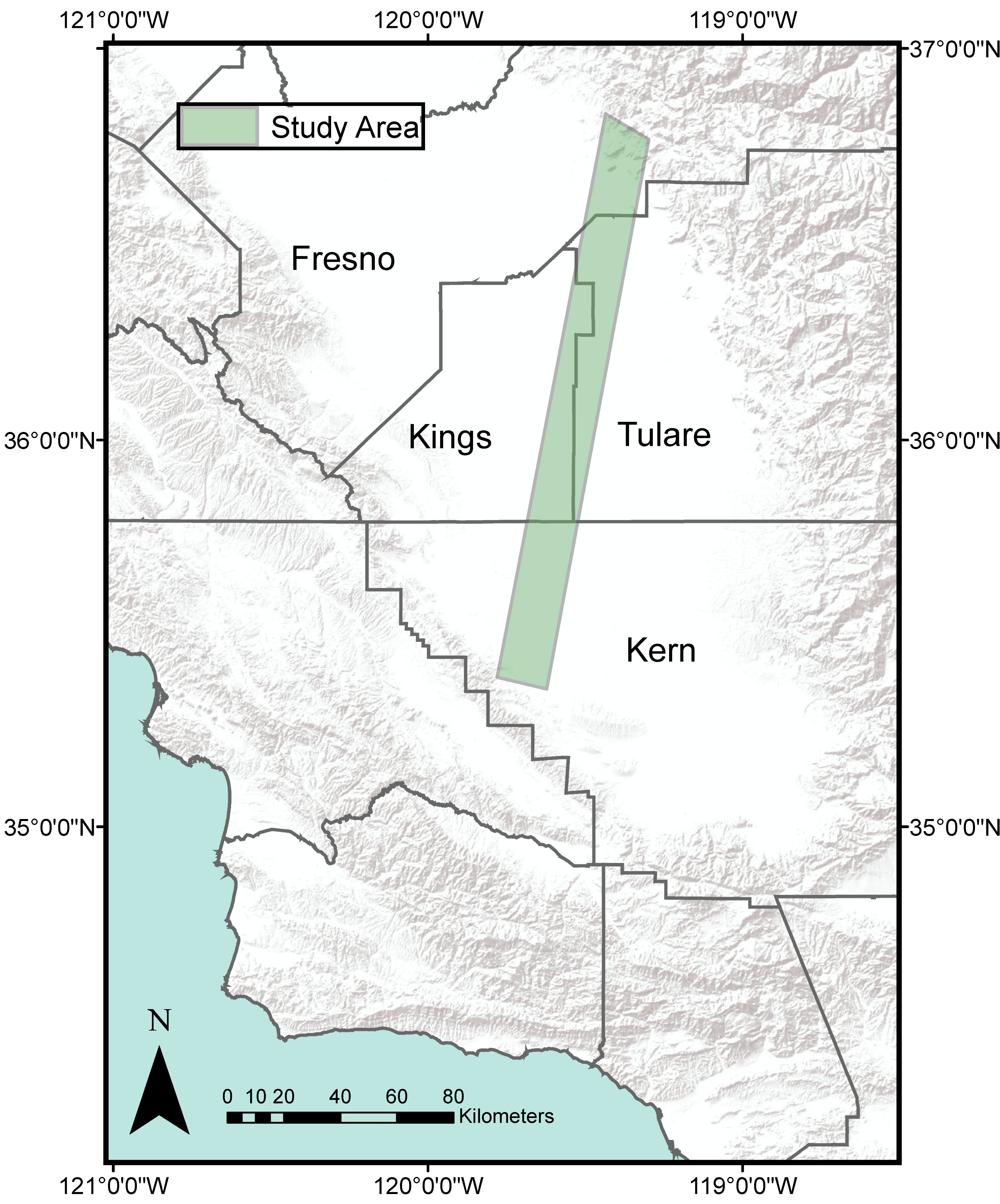
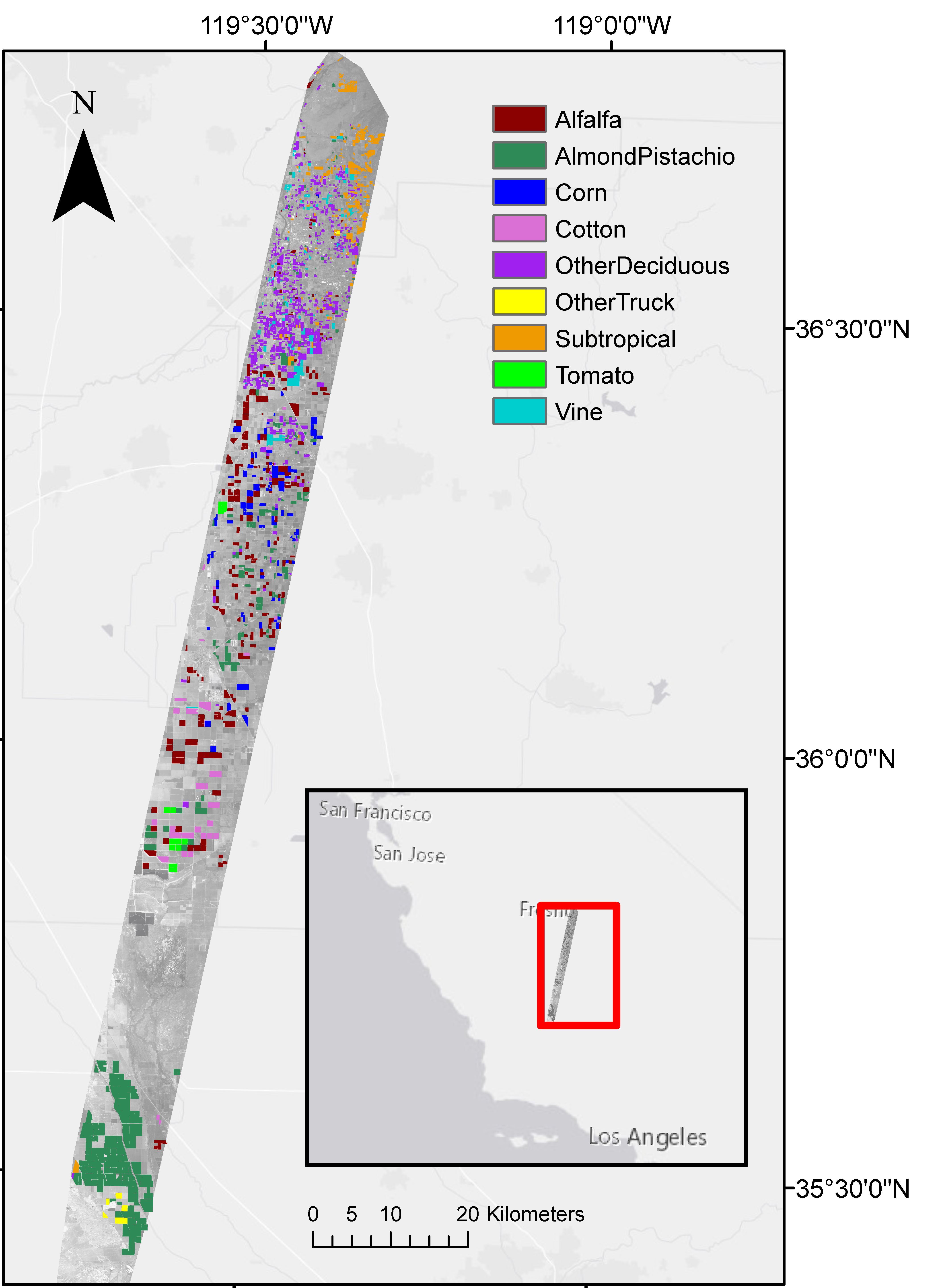
2.1. Study Area
2.2. Datasets
2.2.1. Imagery
2.2.2. Crop Polygons
2.3. Spectral Mixture Analysis
2.4. Classification
2.4.1. Class Selection
2.4.2. Random Forest
2.4.3. Field-Level Reclassification
2.5. Accuracy Assessments
2.5.1. Multispectral Imager Comparisons
2.5.2. Portability Analysis
2.6. Case Study on Farmer Decision-Making
3. Results
3.1. Classification Accuracy
3.1.1. Out-of-Bag Accuracy
3.1.2. Independent Validation
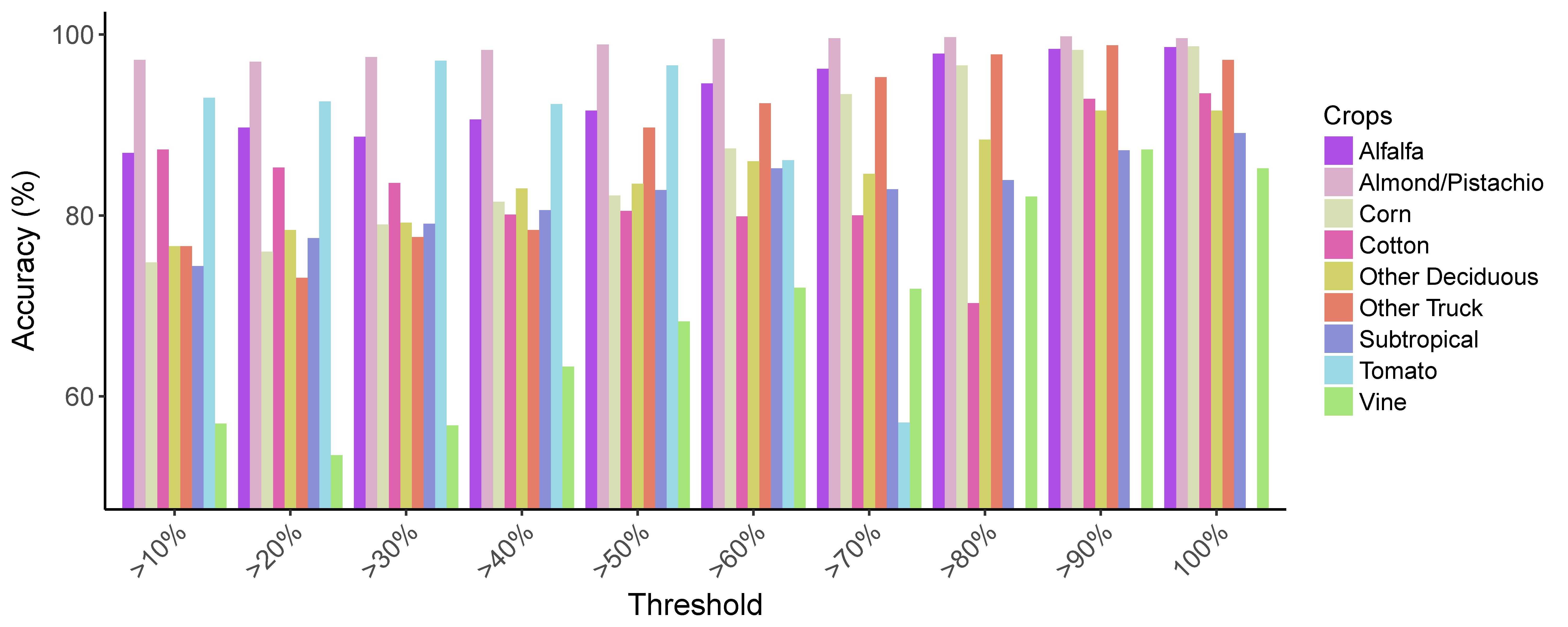
3.1.3. Field-Level Validation after Majority Filter
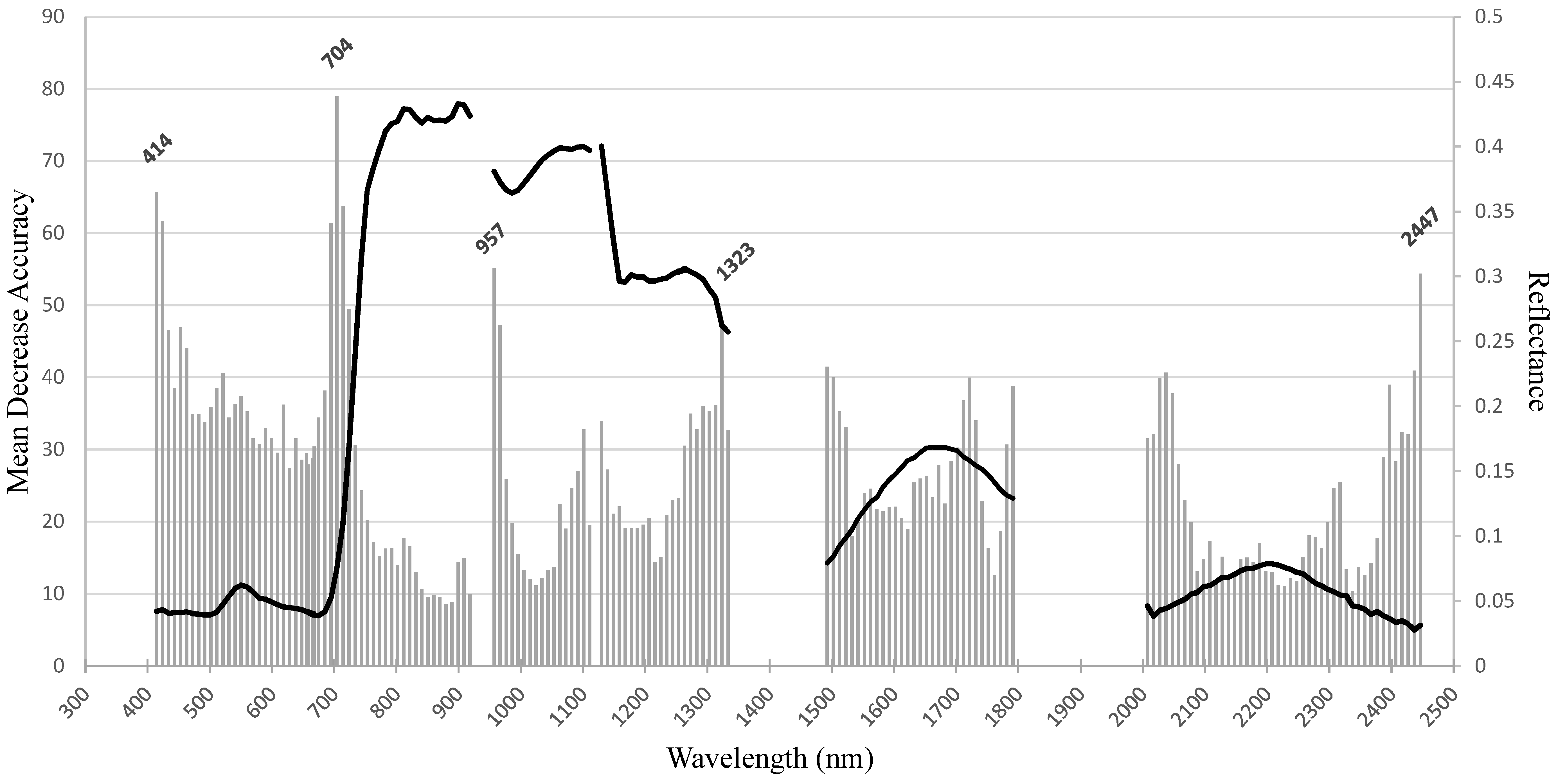
3.1.4. Band Importance
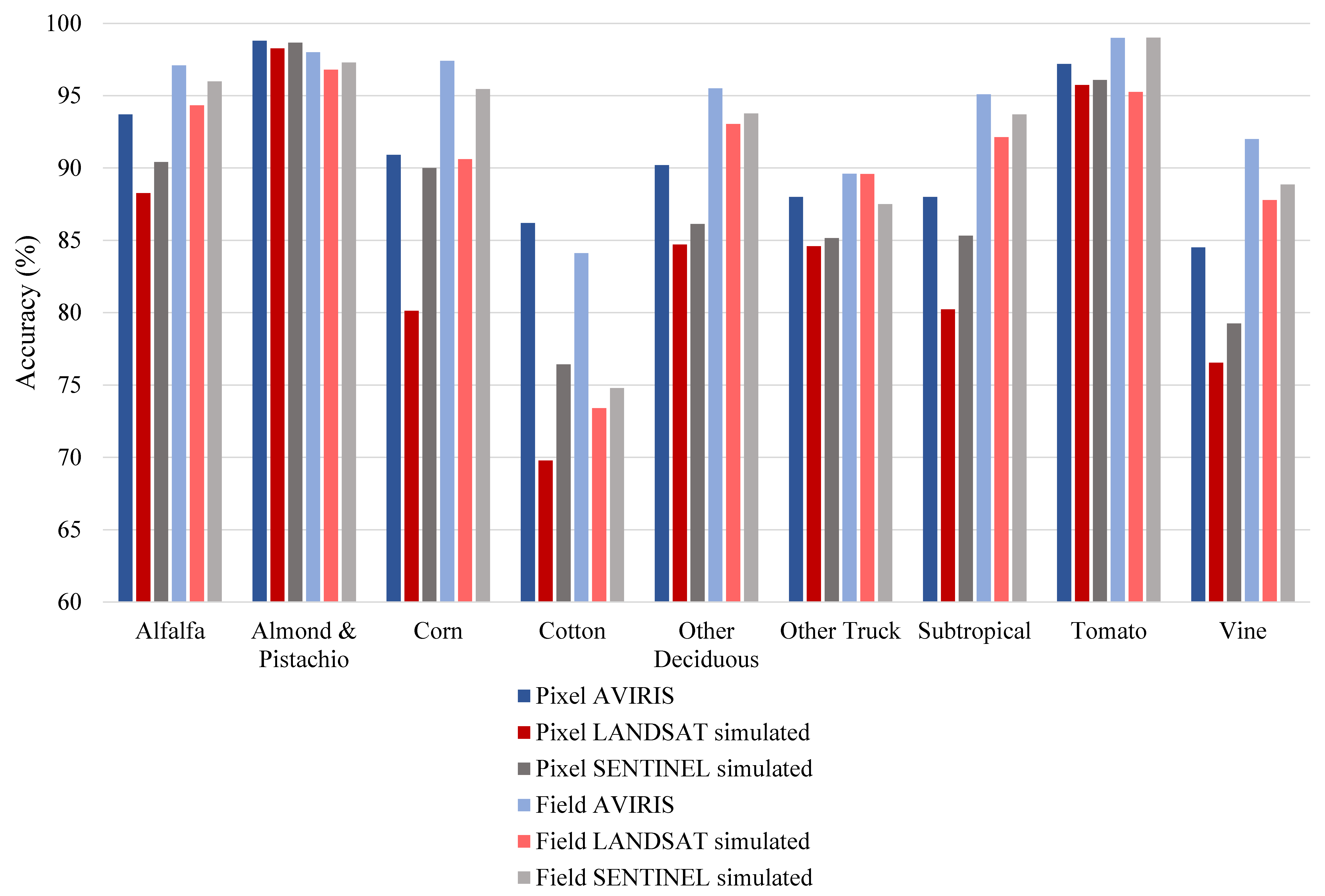
3.1.5. Landsat and Sentinel Comparisons
3.1.6. Portability Assessment
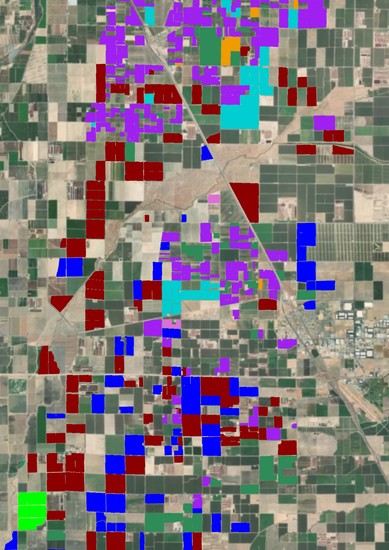
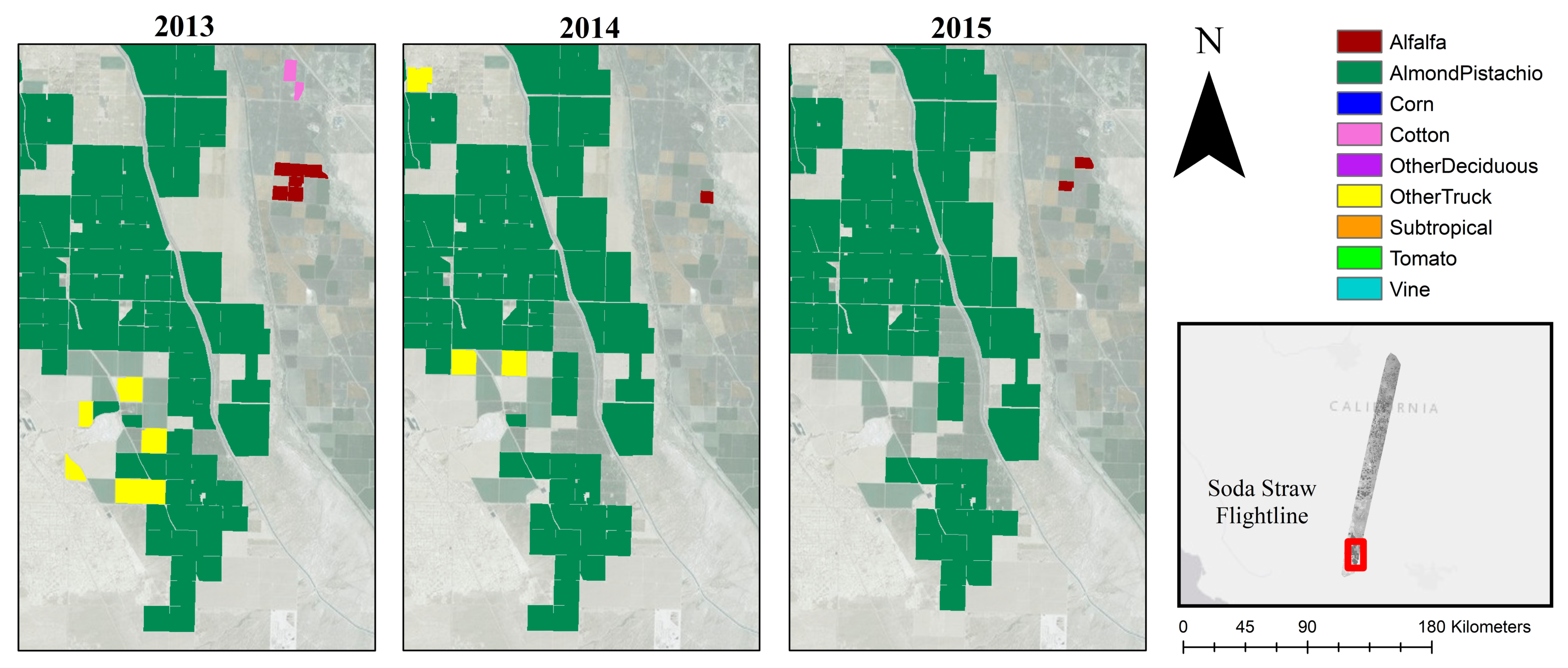
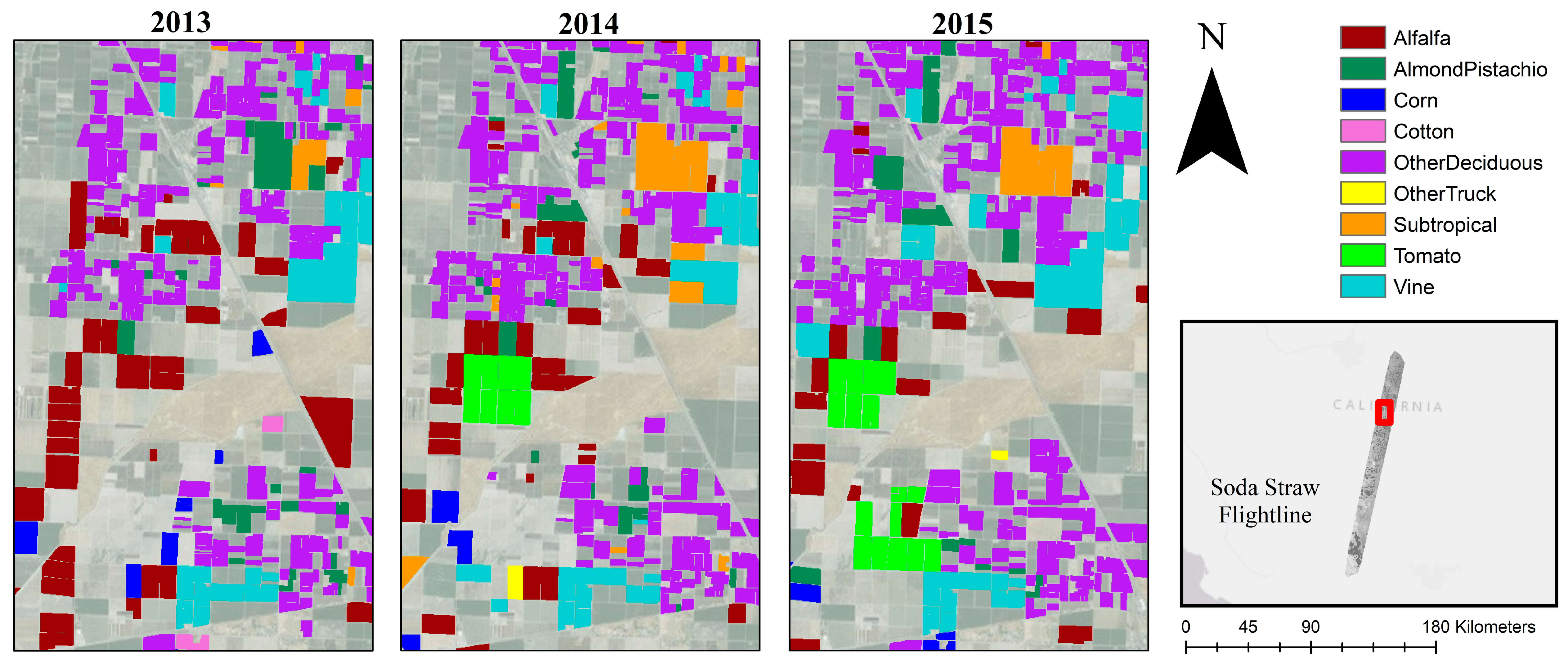
3.2. Central Valley Case Study: Changes in Cropping Patterns
3.3. Central Valley Case Study: Crop Area in Relation to Environmental and Economic Drivers
4. Discussion
4.1. Challenges and Caveats
4.2. Crop Classification with Imaging Spectroscopy
4.3. Implications for Agricultural Management
5. Conclusions
Supplementary Materials
Author Contributions
Funding
Acknowledgments
Conflicts of Interest
References
- Diffenbaugh, N.S.; Swain, D.L.; Touma, D. Anthropogenic warming has increased drought risk in California. Proc. Natl. Acad. Sci. USA 2015, 112, 3931–3936. [Google Scholar] [CrossRef] [PubMed]
- Griffin, D.; Anchukaitis, K.J. How unusual is the 2012–2014 California drought? Geophys. Res. Lett. 2014, 41, 9017–9023. [Google Scholar] [CrossRef]
- Swain, D.L.; Tsiang, M.; Haugen, M.; Singh, D.; Charland, A.; Rajaratnam, B.; Diffenbaugh, N.S. The extraordinary California drought of 2013/2014: Character, context, and the role of climate change. Bull. Am. Meteorol. Soc. 2014, 95, S3–S7. [Google Scholar]
- AghaKouchak, A.; Cheng, L.; Mazdiyasni, O.; Farahmand, A. Global warming and changes in risk of concurrent climate extremes: Insights from the 2014 California drought. Geophys. Res. Lett. 2014, 41, 8847–8852. [Google Scholar] [CrossRef]
- AghaKouchak, A.; Feldman, D.; Hoerling, M.; Huxman, T.; Lund, J. Water and climate: Recognize anthropogenic drought. Nature 2015, 524, 409. [Google Scholar] [CrossRef] [PubMed]
- Howden, S.M.; Soussana, J.F.; Tubiello, F.N.; Chhetri, N.; Dunlop, M.; Meinke, H. Adapting agriculture to climate change. Proc. Natl. Acad. Sci. USA 2007, 104, 19691–19696. [Google Scholar] [CrossRef] [PubMed]
- Lobell, D.B.; Burke, M.B.; Tebaldi, C.; Mastrandrea, M.D.; Falcon, W.P.; Naylor, R.L. Prioritizing climate change adaptation needs for food security in 2030. Science 2008, 319, 607–610. [Google Scholar] [CrossRef] [PubMed]
- Palazzo, J.; Liu, O.R.; Stillinger, T.; Song, R.; Wang, Y.; Hiroyasu, E.; Zenteno, J.; Anderson, S.; Tague, C. Urban responses to restrictive conservation policy during drought. Water Resour. Res. 2017, 53, 4459–4475. [Google Scholar] [CrossRef]
- Agricultural Water Use Efficiency. Available online: https://water.ca.gov/Programs/Water-Use-And-Efficiency/Agricultural-Water-Use-Efficiency (accessed on 10 July 2018).
- Lobell, D.B.; Field, C.B.; Cahill, K.N.; Bonfils, C. Impacts of future climate change on California perennial crop yields: Model projections with climate and crop uncertainties. Agric. For. Meteorol. 2006, 141, 208–218. [Google Scholar] [CrossRef]
- Schlenker, W.; Hanemann, W.M.; Fisher, A.C. Water availability, degree days, and the potential impact of climate change on irrigated agriculture in California. Clim. Chang. 2007, 81, 19–38. [Google Scholar] [CrossRef]
- Medellín-Azuara, J.; Harou, J.J.; Olivares, M.A.; Madani, K.; Lund, J.R.; Howitt, R.E.; Tanaka, S.K.; Jenkins, M.W.; Zhu, T. Adaptability and adaptations of California’s water supply system to dry climate warming. Clim. Chang. 2008, 87, 75–90. [Google Scholar] [CrossRef]
- Tanaka, S.K.; Zhu, T.; Lund, J.R.; Howitt, R.E.; Jenkins, M.W.; Pulido, M.A.; Tauber, M.; Ritzema, R.; Ferreira, I.C. Climate warming and water management adaptation for California. Clim. Chang. 2006, 76, 361–387. [Google Scholar] [CrossRef]
- Vermeulen, S.J.; Aggarwal, P.K.; Ainslie, A.; Angelone, C.; Campbell, B.M.; Challinor, A.J.; Hansen, J.; Ingram, J.S.; Jarvis, A.; Kristjanson, P.; et al. Agriculture, Food Security and Climate Change: Outlook for Knowledge, Tools and Action. Climate Change, Agriculture and Food Security Report 3; CGIAR-ESSP Program on Climate Change, Agriculture and Food Security (CCAFS): Copenhagen, Denmark, 2010. [Google Scholar]
- Adams, R.M.; Rosenzweig, C.; Peart, R.M.; Ritchie, J.T.; McCarl, B.A.; Glyer, J.D.; Curry, R.B.; Jones, J.W.; Boote, K.J.; Allen, L.H. Global climate change and US agriculture. Nature 1990, 345, 219–224. [Google Scholar] [CrossRef]
- Challinor, A.J.; Watson, J.; Lobell, D.B.; Howden, S.M.; Smith, D.R.; Chhetri, N. A meta-analysis of crop yield under climate change and adaptation. Nat. Clim. Chang. 2014, 4, 287–291. [Google Scholar] [CrossRef]
- Tortajada, C.; Kastner, M.J.; Buurman, J.; Biswas, A.K. The California drought: Coping responses and resilience building. Environ. Sci. Policy 2017, 78, 97–113. [Google Scholar] [CrossRef]
- Allen, R.G.; Pereira, L.S.; Raes, D.; Smith, M. FAO Irrigation and Drainage Paper No. 56; Food and Agriculture Organization of the United Nations: Rome, Italy, 1998; Volume 56, pp. 26–40. [Google Scholar]
- California Department of Food and Agriculture. California Agricultural Statistics Review 2014–2015. Available online: https://www.cdfa.ca.gov/statistics/PDFs/2015Report.pdf (accessed on 10 July 2018).
- Nuckols, J.R.; Gunier, R.B.; Riggs, P.; Miller, R.; Reynolds, P.; Ward, M.H. Linkage of the California Pesticide Use Reporting Database with spatial land use data for exposure assessment. Environ. Health Perspect. 2007, 115, 684. [Google Scholar] [CrossRef] [PubMed]
- Galvão, L.S.; Epiphanio, J.C.; Breunig, F.M.; Formaggio, A.R. Crop type discrimination using Hyperspectral data. In Hyperspectral Remote Sensing of Vegetation; Thenkabail, P.S., Lyon, J.G., Huete, A., Eds.; CRC Press: Boca Raton, FL, USA, 2016. [Google Scholar]
- Craig, M.E. The NASS cropland data layer program. In Proceedings of the Third International Conference on Geospatial Information in Agriculture and Forestry, Denver, CO, USA, 5–7 November 2001; pp. 5–7. [Google Scholar]
- Lobell, D.B.; Asner, G.P. Cropland distributions from temporal unmixing of MODIS data. Remote Sens. Environ. 2004, 93, 412–422. [Google Scholar] [CrossRef]
- Massey, R.; Sankey, T.T.; Congalton, R.G.; Yadav, K.; Thenkabail, P.S.; Ozdogan, M.; Meador, A.J. MODIS phenology-derived, multi-year distribution of conterminous US crop types. Remote Sens. Environ. 2017, 198, 490–503. [Google Scholar] [CrossRef]
- Ozdogan, M. The spatial distribution of crop types from MODIS data: Temporal unmixing using Independent Component Analysis. Remote Sens. Environ. 2010, 114, 1190–1204. [Google Scholar] [CrossRef]
- Wardlow, B.D.; Egbert, S.L. Large-area crop mapping using time-series MODIS 250 m NDVI data: An assessment for the US Central Great Plains. Remote Sens. Environ. 2008, 112, 1096–1116. [Google Scholar] [CrossRef]
- Yan, L.; Roy, D.P. Conterminous United States crop field size quantification from multi-temporal Landsat data. Remote Sens. Environ. 2016, 172, 67–86. [Google Scholar] [CrossRef]
- Zhong, L.; Hawkins, T.; Biging, G.; Gong, P. A phenology-based approach to map crop types in the San Joaquin Valley, California. Int. J. Remote Sens. 2011, 32, 7777–7804. [Google Scholar] [CrossRef]
- USDA-NASS. United States Department of Agriculture (USDA) National Agricultural Statistics Service Cropland Data Layer. Available online: http://nassgeodata.gmu.edu/CropScape (accessed on 8 June 2018).
- Chang, J.; Hansen, M.C.; Pittman, K.; Carroll, M.; DiMiceli, C. Corn and soybean mapping in the United States using MODIS time-series data sets. Agron. J. 2007, 99, 1654–1664. [Google Scholar] [CrossRef]
- Zhang, X.; Friedl, M.A.; Schaaf, C.B.; Strahler, A.H.; Hodges, J.C.; Gao, F.; Reed, B.C.; Huete, A. Monitoring vegetation phenology using MODIS. Remote Sens. Environ. 2003, 84, 471–475. [Google Scholar] [CrossRef]
- Key, T.; Warner, T.A.; McGraw, J.B.; Fajvan, M.A. A comparison of multispectral and multitemporal information in high spatial resolution imagery for classification of individual tree species in a temperate hardwood forest. Remote Sens. Environ. 2001, 75, 100–112. [Google Scholar] [CrossRef]
- Mariotto, I.; Thenkabail, P.S.; Huete, A.; Slonecker, E.T.; Platonov, A. Hyperspectral versus multispectral crop-productivity modeling and type discrimination for the HyspIRI mission. Remote Sens. Environ. 2013, 139, 291–305. [Google Scholar] [CrossRef]
- Thenkabail, P.S.; Smith, R.B.; De Pauw, E. Evaluation of narrowband and broadband vegetation indices for determining optimal hyperspectral wavebands for agricultural crop characterization. Photogramm. Eng. Remote Sens. 2002, 68, 607–622. [Google Scholar]
- Thenkabail, P.S.; Enclona, E.A.; Ashton, M.S.; Van Der Meer, B. Accuracy assessments of hyperspectral waveband performance for vegetation analysis applications. Remote Sens. Environ. 2004, 91, 354–376. [Google Scholar] [CrossRef]
- Thenkabail, P.S.; Mariotto, I.; Gumma, M.K.; Middleton, E.M.; Landis, D.R.; Huemmrich, K.F. Selection of hyperspectral narrowbands (HNBs) and composition of hyperspectral twoband vegetation indices (HVIs) for biophysical characterization and discrimination of crop types using field reflectance and Hyperion/EO-1 data. IEEE J. Sel. Top. Appl. Earth Obs. Remote Sens. 2013, 6, 427–439. [Google Scholar] [CrossRef]
- Bandos, T.V.; Bruzzone, L.; Camps-Valls, G. Classification of hyperspectral images with regularized linear discriminant analysis. IEEE Trans. Geosci. Remote Sens. 2009, 47, 862–873. [Google Scholar] [CrossRef]
- Camps-Valls, G.; Gómez-Chova, L.; Calpe-Maravilla, J.; Soria-Olivas, E.; Martín-Guerrero, J.D.; Moreno, J. Support vector machines for crop classification using hyperspectral data. In Pattern Recognition and Image Analysis; Springer: Berlin/Heidelberg, Germany, 2003; pp. 134–141. [Google Scholar]
- Galvão, L.S.; Formaggio, A.R.; Tisot, D.A. Discrimination of sugarcane varieties in Southeastern Brazil with EO-1 Hyperion data. Remote Sens. Environ. 2005, 94, 523–534. [Google Scholar] [CrossRef]
- Galvão, L.S.; Roberts, D.A.; Formaggio, A.R.; Numata, I.; Breunig, F.M. View angle effects on the discrimination of soybean varieties and on the relationships between vegetation indices and yield using off-nadir Hyperion data. Remote Sens. Environ. 2009, 113, 846–856. [Google Scholar] [CrossRef]
- Rao, N.R. Development of a crop-specific spectral library and discrimination of various agricultural crop varieties using hyperspectral imagery. Int. J. Remote Sens. 2008, 29, 131–144. [Google Scholar] [CrossRef]
- California Water Plan. Update 2009. Volume 3, Regional Reports. Bulletin 160–09; Department of Water Resources: Sacramento, CA, USA, 2009.
- Carle, D. Introduction to Water in California; University of California Press: Los Angeles, CA, USA, 2004. [Google Scholar]
- Green, R.O.; Eastwood, M.L.; Sarture, C.M.; Chrien, T.G.; Aronsson, M.; Chippendale, B.J.; Faust, J.A.; Pavri, B.E.; Chovit, C.J.; Solis, M.; et al. Imaging spectroscopy and the airborne visible/infrared imaging spectrometer (AVIRIS). Remote Sens. Environ. 1998, 65, 227–248. [Google Scholar] [CrossRef]
- Thompson, D.R.; Gao, B.C.; Green, R.O.; Roberts, D.A.; Dennison, P.E.; Lundeen, S.R. Atmospheric correction for global mapping spectroscopy: ATREM advances for the HyspIRI preparatory campaign. Remote Sens. Environ. 2015, 167, 64–77. [Google Scholar] [CrossRef]
- Lee, C.M.; Cable, M.L.; Hook, S.J.; Green, R.O.; Ustin, S.L.; Mandl, D.J.; Middleton, E.M. An introduction to the NASA Hyperspectral InfraRed Imager (HyspIRI) mission and preparatory activities. Remote Sens. Environ. 2015, 167, 6–19. [Google Scholar] [CrossRef]
- USGS. 2012–2016 California Drought: Historical Perspective. Available online: https://ca.water.usgs.gov/california-drought/california-drought-comparisons.html (accessed on 8 June 2018).
- Robeson, S.M. Revisiting the recent California drought as an extreme value. Geophys. Res. Lett. 2015, 42, 6771–6779. [Google Scholar] [CrossRef]
- United States Drought Monitor. Available online: https://droughtmonitor.unl.edu/ (accessed on 8 June 2018).
- Roberts, D.A.; Gardner, M.; Church, R.; Ustin, S.; Scheer, G.; Green, R.O. Mapping chaparral in the Santa Monica Mountains using multiple endmember spectral mixture models. Remote Sens. Environ. 1998, 65, 267–279. [Google Scholar] [CrossRef]
- Adams, J.B.; Smith, M.O.; Gillespie, A.R. Imaging spectroscopy: Interpretation based on spectral mixture analysis. Remote Geochem. Anal. Elem. Mineral. Compos. 1993, 7, 145–166. [Google Scholar]
- Agricultural Land & Water Use Estimates. Available online: https://water.ca.gov/Programs/Water-Use-And-Efficiency/Land-And-Water-Use/Agricultural-Land-And-Water-Use-Estimates (accessed on 10 July 2018).
- Breiman, L. Random Forests. Mach. Learn. 2001, 45, 5–32. [Google Scholar] [CrossRef]
- Gislason, P.O.; Benediktsson, J.A.; Sveinsson, J.R. Random Forests for land cover classification. Pattern Recognit. Lett. 2006, 27, 294–300. [Google Scholar] [CrossRef]
- Pal, M. Random Forest classifier for remote sensing classification. Int. J. Remote Sens. 2005, 26, 217–222. [Google Scholar] [CrossRef]
- Millard, K.; Richardson, M. On the importance of training data sample selection in random forest image classification: A case study in peatland ecosystem mapping. Remote Sens. 2015, 7, 8489–8515. [Google Scholar] [CrossRef]
- Foody, G.M.; Cox, D.P. Sub-pixel land cover composition estimation using a linear mixture model and fuzzy membership functions. Remote Sens. 1994, 15, 619–631. [Google Scholar] [CrossRef]
- Foody, G.M.; Mathur, A. The use of small training sets containing mixed pixels for accurate hard image classification: Training on mixed spectral responses for classification by a SVM. Remote Sens. Environ. 2006, 103, 179–189. [Google Scholar] [CrossRef]
- CCGGA. California Cotton Information. Available online: https://ccgga.org/cotton-information (accessed on 10 July 2018).
- Pinter, P.J., Jr.; Hatfield, J.L.; Schepers, J.S.; Barnes, E.M.; Moran, M.S.; Daughtry, C.S.; Upchurch, D.R. Remote sensing for crop management. Photogramm. Eng. Remote Sens. 2003, 69, 647–664. [Google Scholar] [CrossRef]
- Foody, G.M. Status of land cover classification accuracy assessment. Remote Sens. Environ. 2002, 80, 185–201. [Google Scholar] [CrossRef]
- Johnson, D.M. A 2010 map estimate of annually tilled cropland within the conterminous United States. Agric. Syst. 2013, 114, 95–105. [Google Scholar] [CrossRef]
- Alcantara, C.; Kuemmerle, T.; Prishchepov, A.V.; Radeloff, V.C. Mapping abandoned agriculture with multi-temporal MODIS satellite data. Remote Sens. Environ. 2012, 124, 334–347. [Google Scholar] [CrossRef]
- Wu, Z.; Thenkabail, P.S.; Mueller, R.; Zakzeski, A.; Melton, F.; Johnson, L.; Rosevelt, C.; Dwyer, J.; Jones, J.; Verdin, J.P. Seasonal cultivated and fallow cropland mapping using MODIS-based automated cropland classification algorithm. J. Appl. Remote Sens. 2014, 8, 083685. [Google Scholar] [CrossRef]
- Clark, M.L. Comparison of simulated hyperspectral HyspIRI and multispectral Landsat 8 and Sentinel-2 imagery for multi-seasonal, regional land-cover mapping. Remote Sens. Environ. 2017, 200, 311–325. [Google Scholar] [CrossRef]
- Platt, R.V.; Goetz, A.F. A comparison of AVIRIS and Landsat for land use classification at the urban fringe. Photogramm. Eng. Remote Sens. 2004, 70, 813–819. [Google Scholar] [CrossRef]
- Clark, M.L.; Roberts, D.A. Species-level differences in hyperspectral metrics among tropical rainforest trees as determined by a tree-based classifier. Remote Sens. 2012, 4, 1820–1855. [Google Scholar] [CrossRef]
- Horler, D.N.; Dockray, M.; Barber, J. The red edge of plant leaf reflectance. Int. J. Remote Sens. 1983, 4, 273–288. [Google Scholar] [CrossRef]
- Zarco-Tejada, P.J.; Ustin, S.L.; Whiting, M.L. Temporal and spatial relationships between within-field yield variability in cotton and high-spatial hyperspectral remote sensing imagery. Agron. J. 2005, 97, 641–653. [Google Scholar] [CrossRef]
- Tucker, C.J.; Garratt, M.W. Leaf optical system modeled as a stochastic process. Appl. Opt. 1977, 16, 635–642. [Google Scholar] [CrossRef] [PubMed]
- Immitzer, M.; Vuolo, F.; Atzberger, C. First experience with Sentinel-2 data for crop and tree species classifications in central Europe. Remote Sens. 2016, 8, 166. [Google Scholar] [CrossRef]
- Kakani, V.G.; Reddy, K.R.; Zhao, D.; Sailaja, K. Field crop responses to ultraviolet-B radiation: A review. Agric. For. Meteorol. 2003, 120, 191–218. [Google Scholar] [CrossRef]
- Vuolo, F.; Neuwirth, M.; Immitzer, M.; Atzberger, C.; Ng, W.T. How much does multi-temporal Sentinel-2 data improve crop type classification? Int. J. Appl. Earth Obs. Geoinf. 2018, 72, 122–130. [Google Scholar] [CrossRef]
- Waldhoff, G.; Lussem, U.; Bareth, G. Multi-Data Approach for remote sensing-based regional crop rotation mapping: A case study for the Rur catchment, Germany. Int. J. Appl. Earth Obs. Geoinf. 2017, 61, 55–69. [Google Scholar] [CrossRef]
- Dudley, K.L.; Dennison, P.E.; Roth, K.L.; Roberts, D.A.; Coates, A.R. A multi-temporal spectral library approach for mapping vegetation species across spatial and temporal phenologicalal gradients. Remote Sens. Environ. 2015, 167, 121–134. [Google Scholar] [CrossRef]
- Cooley, H.; Donnelly, K.; Phurisamban, R.; Subramanian, M. Impacts of California’s Ongoing Drought: Agriculture; Pacific Institute: Oakland, CA, USA, 2015. [Google Scholar]
- Howitt, R.; Medellín-Azuara, J.; MacEwan, D.; Lund, J.R.; Sumner, D. Economic Analysis of the 2014 Drought for California Agriculture; University of California Center for Watershed Sciences: Davis, CA, USA, 2014. [Google Scholar]
- Melton, F.; Rosevelt, C.; Guzman, A.; Johnson, L.; Zaragoza, I.; Verdin, J.; Thenkabail, P.; Wallace, C.; Mueller, R.; Willis, P.; et al. Fallowed Area Mapping for Drought Impact Reporting: 2015 Assessment of Conditions in the California Central Valley; NASA Ames Research Center: Mountain View, CA, USA, 2015.
- Medellín-Azuara, J.; MacEwan, D.; Howitt, R.E.; Koruakos, G.; Dogrul, E.C.; Brush, C.F.; Kadir, T.N.; Harter, T.; Melton, F.; Lund, J.R. Hydro-economic analysis of groundwater pumping for irrigated agriculture in California’s Central Valley, USA. Hydrogeol. J. 2015, 23, 1205–1216. [Google Scholar] [CrossRef]
- Hanak, E. Managing California’s Water: From Conflict to Reconciliation; Public Policy Institute of CA: San Francisco, CA, USA, 2011. [Google Scholar]
- Christian-Smith, J.; Levy, M.C.; Gleick, P.H. Maladaptation to drought: A case report from California, USA. Sustain. Sci. 2015, 10, 491–501. [Google Scholar] [CrossRef]


| Crop Class | Definition | Included in Study |
|---|---|---|
| Grain | Wheat, barley, oats, miscellaneous grain and hay, and mixed grain and hay | No |
| Rice | Rice and wild rice | No |
| Cotton | Cotton | Yes |
| Sugar Beet | Sugar beets | No |
| Corn | Corn (field and sweet) | Yes |
| Dry Bean | Beans (dry) | No |
| Safflower | Safflower | No |
| Other Field | Flax, hops, grain sorghum, sudan, castor beans, miscellaneous fields, sunflowers, hybrid sorghum/sudan, millet, and sugar cane | No |
| Alfalfa | Alfalfa and alfalfa mixtures | Yes |
| Pasture | Clover, mixed pasture, native pastures, induced high water table native pasture, miscellaneous grasses, turf farms, bermuda grass, rye grass, and klein grass | No |
| Processing Tomato | Tomatoes for processing | Yes, combined with fresh |
| Fresh Tomato | Tomatoes for market | Yes, combined with processing |
| Cucurbit | Melons, squash, and cucumbers | No |
| Onion Garlic | Onions and garlic | No |
| Potato | Potatoes | No |
| Other Truck Crops | Artichokes, asparagus, beans (green), carrots, celery, lettuce, peas, spinach, flowers nursery and tree farms, bush berries, strawberries, peppers, broccoli, cabbage, cauliflower, and brussels sprouts | Yes |
| Almond Pistachio | Almonds and pistachios | Yes |
| Other Deciduous Crops | Apples, apricots, cherries, peaches, nectarines, pears, plums, prunes, figs, walnuts, and miscellaneous deciduous | Yes |
| Subtropical | Grapefruit, lemons, oranges, dates, avocados, olives, kiwis, jojoba, eucalyptus, and miscellaneous subtropical fruit | Yes |
| Vine | Table grapes, wine grapes, and raisin grapes | Yes |
| Crops | Number of Fields | Total Area (km2) |
|---|---|---|
| Studied Crops | ||
| Alfalfa | 340 | 954.4 |
| Almond/Pistachio | 442 | 3305.3 |
| Corn | 97 | 236.8 |
| Cotton | 22 | 64.6 |
| Other Deciduous Crops | 2174 | 1517.8 |
| Other Truck Crops | 22 | 76.5 |
| Subtropical | 634 | 769.5 |
| Tomato | 29 | 87.6 |
| Vine | 350 | 478.1 |
| Other Crops | ||
| Cucurbit | 3 | 1.1 |
| Grain | 1 | 5.2 |
| Pasture | 8 | 13.7 |
| Safflower | 3 | 21.8 |
| Sugar Beet | 4 | 8.0 |
| Uncultivated | 17 | 15.0 |
| Crops | Out-of-Bag Accuracy | Independent Validation Pixel-Level Accuracy by Year (%) | Field-Level Accuracy after Majority Filter with 50% GV Threshold (%) | ||||
|---|---|---|---|---|---|---|---|
| All Years | 2013 | 2014 | 2015 | 2013 | 2014 | 2015 | |
| Alfalfa | 93.7 | 94.5 | 87.6 | 93.0 | 94.2 | 94.7 | 97.1 |
| Almond and Pistachio | 98.8 | 96.1 | 96.2 | 94.2 | 88.9 | 91.7 | 95.6 |
| Corn | 90.9 | 93.1 | 77.0 | 95.1 | 98.3 | 93.8 | 94.1 |
| Cotton | 86.2 | 73.5 | 45.7 | 21.5 | 73.3 | 83.3 | 85.7 |
| Other Deciduous | 90.2 | 86.1 | 82.6 | 85.0 | 95.6 | 95.3 | 96.6 |
| Other Truck | 88.0 | 76.4 | 78.6 | NA | 100.0 | 100.0 | 68.8 |
| Subtropical | 88.0 | 83.9 | 81.8 | 80.6 | 92.3 | 93.2 | 92.9 |
| Tomato | 97.2 | NA | 92.3 | 89.2 | 100.0 | 100.0 | 97.1 |
| Vine | 84.5 | 77.2 | 70.2 | 83.5 | 88.3 | 90.6 | 93.4 |
| Reference Data | |||||||||||
|---|---|---|---|---|---|---|---|---|---|---|---|
| AF | AP | CR | CT | OD | OT | ST | TO | VI | Total | ||
| Classified | AF | 17,733 | 295 | 8 | 13 | 521 | 4 | 71 | 16 | 256 | 18,917 |
| AP | 34 | 64,449 | 1 | 7 | 497 | 3 | 178 | 8 | 42 | 65,219 | |
| CR | 50 | 126 | 3645 | 17 | 160 | 1 | 3 | 2 | 4 | 4008 | |
| CT | 40 | 88 | 3 | 1347 | 62 | 0 | 5 | 3 | 14 | 1562 | |
| OD | 194 | 1514 | 7 | 11 | 26,821 | 0 | 837 | 12 | 283 | 29,679 | |
| OT | 36 | 23 | 0 | 7 | 111 | 1877 | 12 | 2 | 66 | 2134 | |
| ST | 36 | 694 | 1 | 7 | 1205 | 8 | 15,067 | 5 | 96 | 17,119 | |
| TO | 18 | 14 | 1 | 0 | 3 | 0 | 4 | 1660 | 8 | 1708 | |
| VI | 240 | 212 | 1 | 12 | 858 | 10 | 150 | 8 | 8109 | 9600 | |
| Total | 18,381 | 67,415 | 3667 | 1421 | 30,238 | 1903 | 16,327 | 1716 | 8878 | ||
| User’s Acc. | 93.7% | 98.8% | 90.9% | 86.2% | 90.4% | 88.0% | 88.0% | 97.2% | 84.5% | ||
| Producer’s Acc. | 96.5% | 95.6% | 99.4% | 94.8% | 88.7% | 98.6% | 92.3% | 96.7% | 91.3% | ||
| OOB Acc. | 93.8% | ||||||||||
| Reference Data | |||||||||||
|---|---|---|---|---|---|---|---|---|---|---|---|
| AF | AP | CR | CT | OD | OT | ST | TO | VI | Total | ||
| Classified | AF | 3891 | 12 | 22 | 8 | 52 | 3 | 2 | 43 | 85 | 4118 |
| AP | 66 | 12,395 | 46 | 94 | 313 | 1 | 189 | 5 | 75 | 13,184 | |
| CR | 42 | 1 | 971 | 2 | 13 | 0 | 0 | 0 | 0 | 1029 | |
| CT | 15 | 3 | 13 | 161 | 5 | 3 | 0 | 0 | 2 | 202 | |
| OD | 226 | 256 | 75 | 48 | 5479 | 21 | 305 | 3 | 283 | 6696 | |
| OT | 0 | 0 | 1 | 0 | 4 | 55 | 0 | 0 | 1 | 61 | |
| ST | 45 | 70 | 2 | 5 | 289 | 4 | 2404 | 1 | 145 | 2965 | |
| TO | 9 | 1 | 2 | 0 | 3 | 0 | 1 | 292 | 0 | 308 | |
| VI | 52 | 13 | 2 | 5 | 87 | 10 | 20 | 4 | 1244 | 1437 | |
| Total | 4346 | 12,751 | 1134 | 323 | 6245 | 97 | 2921 | 348 | 1835 | ||
| User’s Acc. | 94.5% | 94.0% | 94.4% | 79.7% | 81.8% | 90.2% | 81.1% | 94.8% | 86.6% | ||
| Producer’s Acc. | 89.5% | 97.2% | 85.6% | 49.8% | 87.7% | 56.7% | 82.3% | 83.9% | 67.8% | ||
| Kappa | 0.86 | ||||||||||
| Overall Acc. | 89.6% | ||||||||||
| Reference Data | |||||||||||
|---|---|---|---|---|---|---|---|---|---|---|---|
| AF | AP | CR | CT | OD | OT | ST | TO | VI | Total | ||
| Classified | AF | 324 | 0 | 1 | 3 | 4 | 0 | 1 | 1 | 4 | 388 |
| AP | 1 | 432 | 2 | 2 | 44 | 0 | 12 | 0 | 5 | 498 | |
| CR | 2 | 0 | 92 | 1 | 1 | 0 | 0 | 0 | 0 | 96 | |
| CT | 1 | 0 | 0 | 15 | 1 | 0 | 0 | 0 | 0 | 17 | |
| OD | 9 | 6 | 2 | 1 | 2095 | 4 | 42 | 0 | 38 | 2197 | |
| OT | 0 | 0 | 0 | 0 | 0 | 17 | 0 | 0 | 0 | 17 | |
| ST | 2 | 4 | 0 | 0 | 24 | 0 | 578 | 0 | 6 | 614 | |
| TO | 0 | 0 | 0 | 0 | 0 | 0 | 0 | 28 | 0 | 28 | |
| VI | 1 | 0 | 0 | 0 | 5 | 1 | 1 | 0 | 297 | 305 | |
| Total | 340 | 442 | 97 | 22 | 2174 | 22 | 634 | 29 | 350 | ||
| User’s Acc. | 95.9% | 86.7% | 95.8% | 88.2% | 95.4% | 100% | 94.1% | 100% | 97.4% | ||
| Producer’s Acc. | 95.3% | 97.7% | 94.8% | 68.2% | 96.4% | 77.3% | 91.2% | 96.6% | 84.9% | ||
| Kappa | 0.91 | ||||||||||
| Overall Acc. | 94.4% | ||||||||||
| Crops | Field-Level Accuracy (%) | Percent Decrease in Accuracy | ||||
|---|---|---|---|---|---|---|
| 2013 Trained on 2014 and 2015 | 2014 Trained on 2013 and 2015 | 2015 Trained on 2013 and 2014 | 2013 | 2014 | 2015 | |
| Alfalfa | 74.7 | 54.1 | 87.4 | 19.5 | 40.6 | 9.7 |
| Almond and Pistachio | 71.1 | 66.7 | 70.5 | 17.8 | 25.0 | 25.1 |
| Corn | 86.7 | 68.8 | 89.9 | 11.6 | 25.1 | 4.2 |
| Cotton | 28.3 | 0 | 32.1 | 45.0 | 83.3 | 53.6 |
| Other Deciduous | 87.0 | 54.1 | 87.3 | 8.6 | 41.2 | 9.3 |
| Other Truck | NA | NA | 0 | NA | NA | 68.8 |
| Subtropical | 78.2 | 62.3 | 66.5 | 14.1 | 30.9 | 26.4 |
| Tomato | 100 | NA | 61.8 | 0 | NA | 35.3 |
| Vine | 71.9 | 61.3 | 78.3 | 16.4 | 29.3 | 15.1 |
| Classified Fields | |
|---|---|
| 2013 | |
| Percent included in validation layer | 39.0% |
| Percent not included in validation layer | 61.0% |
| Total number classified | 3469 |
| 2014 | |
| Percent included in validation layer | 36.4% |
| Percent not included in validation layer | 63.6% |
| Total number classified | 3361 |
| 2015 | |
| Percent included in validation layer | 48.9% |
| Percent not included in validation layer | 51.1% |
| Total number classified | 3235 |
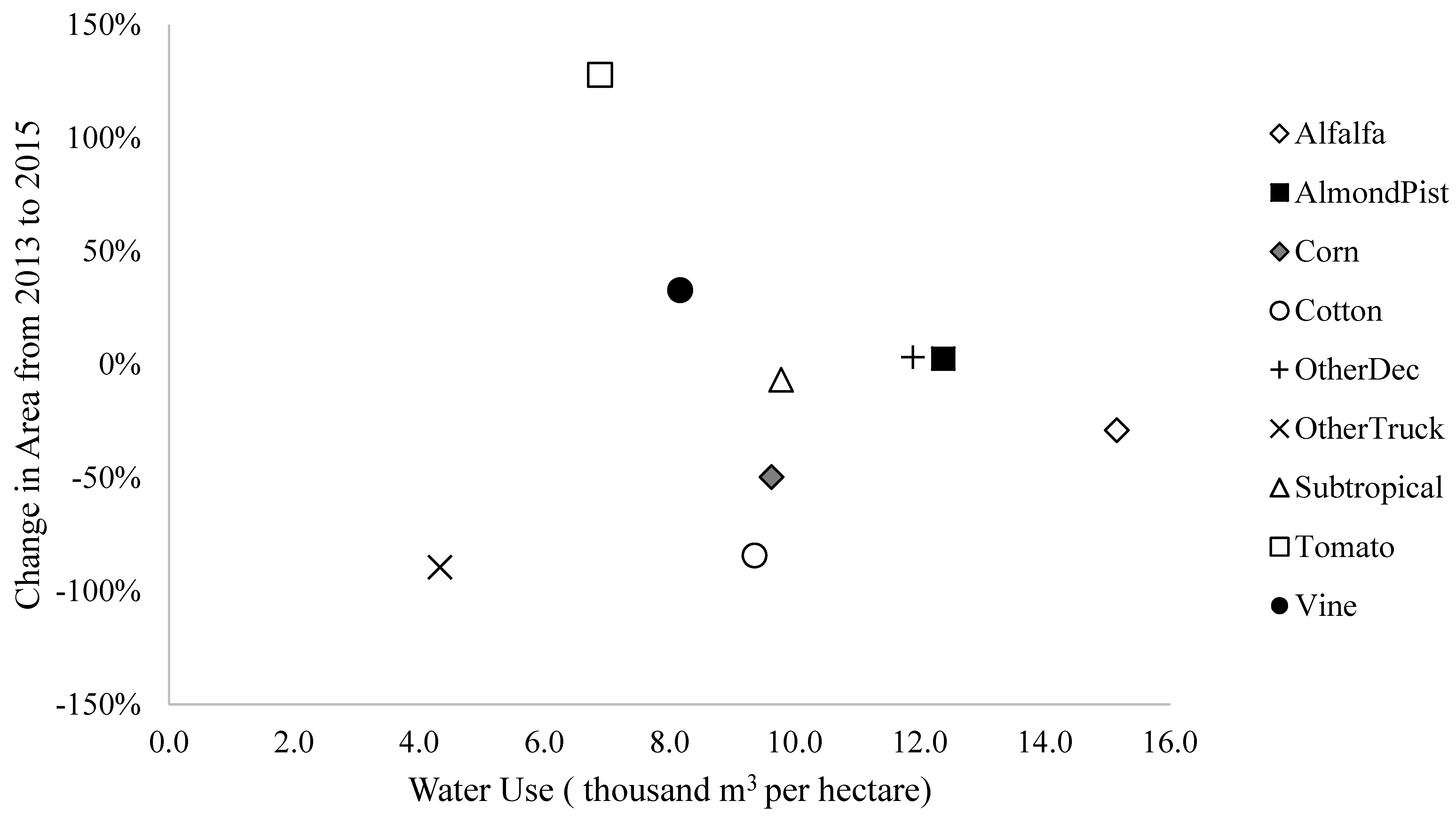
| Crops | Cropland (km2) | Change in Area | ||||
|---|---|---|---|---|---|---|
| 2013 | 2014 | 2015 | 2013 to 2014 | 2014 to 2015 | 2013 to 2015 | |
| Alfalfa | 68.6 | 57.1 | 48.7 | −16.8% | −14.6% | −28.9% |
| Almond and Pistachio | 124.9 | 131.5 | 128.2 | 5.3% | −2.5% | 2.6% |
| Corn | 25.1 | 14.0 | 12.7 | −44.3% | −9.5% | −49.6% |
| Cotton | 17.2 | 1.5 | 2.7 | −91.4% | 85.4% | −84.1% |
| Other Deciduous | 74.2 | 77.8 | 76.7 | 4.8% | −1.4% | 3.4% |
| Other Truck | 3.4 | 3.4 | 0.4 | 0.3% | −89.4% | −89.4% |
| Subtropical | 26.6 | 34.7 | 24.9 | 30.3% | −28.4% | −6.7% |
| Tomato | 6.9 | 5.7 | 15.8 | −18.0% | 178.2% | 128.0% |
| Vine | 16.0 | 17.7 | 21.2 | 11.0% | 19.7% | 32.9% |
| Total | 362.9 | 343.3 | 331.2 | −5.4% | −3.5% | −8.7% |
| Average Water Application per Hectare (Thousand m3) | Total Water Application (km3 Multiplied by 1000) Calculated with the Classification Maps | |||
|---|---|---|---|---|
| 2013 | 2014 | 2015 | ||
| Alfalfa | 15.1 | 103.9 | 86.5 | 73.8 |
| Almond and Pistachio | 12.4 | 154.6 | 162.7 | 158.7 |
| Corn | 9.6 | 24.2 | 13.5 | 12.2 |
| Cotton | 9.4 | 16.1 | 1.4 | 2.6 |
| Other Deciduous | 11.9 | 88.2 | 92.4 | 91.2 |
| Other Truck | 4.3 | 1.5 | 1.5 | 0.2 |
| Subtropical | 9.8 | 26.1 | 33.9 | 24.3 |
| Tomato | 6.9 | 4.8 | 3.9 | 10.9 |
| Vine | 8.2 | 13.0 | 14.5 | 17.3 |
| Total | 432.3 | 410.3 | 391.1 | |
© 2018 by the authors. Licensee MDPI, Basel, Switzerland. This article is an open access article distributed under the terms and conditions of the Creative Commons Attribution (CC BY) license (http://creativecommons.org/licenses/by/4.0/).
Share and Cite
Shivers, S.W.; Roberts, D.A.; McFadden, J.P.; Tague, C. Using Imaging Spectrometry to Study Changes in Crop Area in California’s Central Valley during Drought. Remote Sens. 2018, 10, 1556. https://doi.org/10.3390/rs10101556
Shivers SW, Roberts DA, McFadden JP, Tague C. Using Imaging Spectrometry to Study Changes in Crop Area in California’s Central Valley during Drought. Remote Sensing. 2018; 10(10):1556. https://doi.org/10.3390/rs10101556
Chicago/Turabian StyleShivers, Sarah W., Dar A. Roberts, Joseph P. McFadden, and Christina Tague. 2018. "Using Imaging Spectrometry to Study Changes in Crop Area in California’s Central Valley during Drought" Remote Sensing 10, no. 10: 1556. https://doi.org/10.3390/rs10101556
APA StyleShivers, S. W., Roberts, D. A., McFadden, J. P., & Tague, C. (2018). Using Imaging Spectrometry to Study Changes in Crop Area in California’s Central Valley during Drought. Remote Sensing, 10(10), 1556. https://doi.org/10.3390/rs10101556