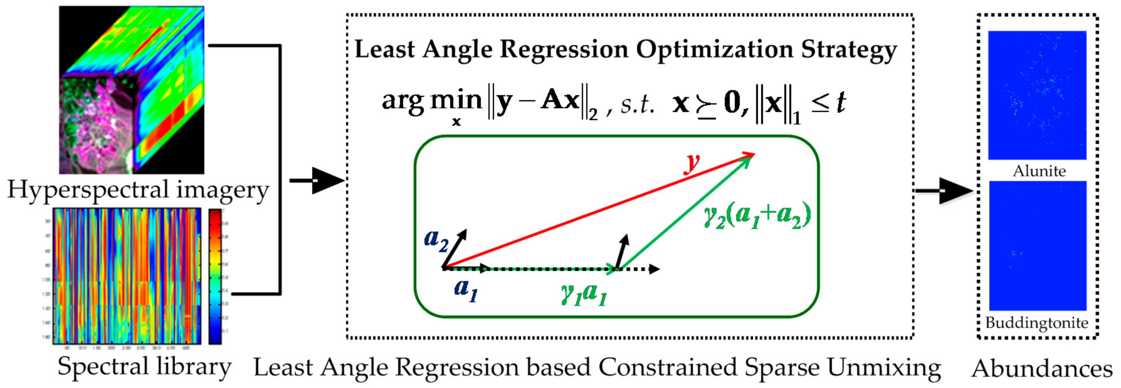
Least Angle Regression-Based Constrained Sparse Unmixing of Hyperspectral Remote Sensing Imagery

Abstract

Sparse unmixing has been successfully applied in hyperspectral remote sensing imagery analysis based on a standard spectral library known in advance. This approach involves reformulating the traditional linear spectral unmixing problem by finding the optimal subset of signatures in this spectral library using the sparse regression technique, and has greatly improved the estimation of fractional abundances in ubiquitous mixed pixels. Since the potentially large standard spectral library can be given a priori, the most challenging task is to compute the regression coefficients, i.e., the fractional abundances, for the linear regression problem. There are many mathematical techniques that can be used to deal with the spectral unmixing problem; e.g., ordinary least squares (OLS), constrained least squares (CLS), orthogonal matching pursuit (OMP), and basis pursuit (BP). However, due to poor prediction accuracy and non-interpretability, the traditional methods often cannot obtain satisfactory estimations or achieve a reasonable interpretation. In this paper, to improve the regression accuracy of sparse unmixing, least angle regression-based constrained sparse unmixing (LARCSU) is introduced to further enhance the precision of sparse unmixing. Differing from the classical greedy algorithms and some of the cautious sparse regression-based approaches, the LARCSU algorithm has two main advantages. Firstly, it introduces an equiangular vector to seek the optimal regression steps based on the simple underlying geometry. Secondly, unlike the alternating direction method of multipliers (ADMM)-based algorithms that introduce one or more multipliers or augmented terms during their optimization procedures, no parameters are required in the computational process of the LARCSU approach. The experimental results obtained with both simulated datasets and real hyperspectral images confirm the effectiveness of LARCSU compared with the current state-of-the-art spectral unmixing algorithms. LARCSU can obtain a better fractional abundance map, as well as a higher unmixing accuracy, with the same order of magnitude of computational effort as the CLS-based methods.

1. Introduction

Hyperspectral unmixing is one of the most important research topics in applied remote sensing imagery processing, since mixed pixels are widely encountered in remote sensing imagery [1,2,3,4,5]. Spectral unmixing is an effective way to analyze and quantify mixed pixels by estimating all the pure materials (endmembers) and computing the corresponding fractional abundances [6,7,8]. Based on the different observation model assumptions, most spectral unmixing algorithms can be divided into two categories: linear-mixture-based models and nonlinear-mixture-based models [2,7,8]. As a result of its computational tractability and flexibility in different applications, as well as its feasibility in most macroscopic remote sensing scenarios, the linear mixture assumption is usually adopted in most hyperspectral unmixing analyses [9,10,11,12]. For this reason, in this paper, we study the linear spectral unmixing model.

In the linear mixture model, given a set of observed mixed hyperspectral remote sensing pixels, denoted as y, spectral unmixing is aimed at estimating the fractional abundances (denoted as x) of the pure spectral signatures (called “endmembers” and denoted as M). The expression can be written as follows:

$$\mathbf{y}=\mathbf{M}\mathbf{x}+\mathbf{n}$$

(1)

where y = (y₁, y₂, …, y_L)^T is a mixed pixel with L bands, and $\mathbf{M}\in {\mathbf{R}}^{L\times q}$ denotes the spectral signatures’ matrix containing q endmembers. The n used in Equation (1) means the existence of noise or modeling errors. Considering the physical constraint that each mixed pixel should obey, the abundance non-negative constraint (ANC) is enforced in the original linear mixture model, which can be expressed as:

$$\mathbf{y}=\mathbf{M}\mathbf{x}+\mathbf{n} s.t. \mathbf{x}\underset{\_}{\succ }0$$

(2)

Since y is the observed hyperspectral remote sensing image pixel data, which can be treated as a vector, the traditional spectral unmixing methods usually estimate the endmembers’ signatures with y under a simple assumption model [13,14,15,16], such as the pixel purity index (PPI) [13], N-FINDR [14], or vertex component analysis (VCA) [15], and identify the endmembers located at the vertices of the whole dataset simplex to decide M. The spectral unmixing then becomes a regression problem: we have data (M, y) and wish to recover a vector, or fractional abundance, $\mathbf{x}\in {\mathbf{R}}^{q\times 1}$. To cope with this linear regression problem, many mathematical methods can be used, such as ordinary least squares (OLS), which is widely known and used as the basic idea for fully constrained least squares (FCLS) in spectral unmixing [9]. In addition, optimal band analysis for the normalized difference water index (OBA-NDWI) has been proposed for the precise estimation of the water fraction [17], and normalized difference vegetation index (NDVI)-based regression has been used for the estimation of vegetation abundance [18]. However, due to poor prediction accuracy and non-interpretability, OLS-based fractional abundance inversion often cannot obtain satisfactory estimations or exhibit a reasonable interpretation.

In recent years, sparse unmixing has been proposed as a semi-supervised spectral unmixing method, supposing that the observed hyperspectral imagery can be expressed in the form of a linear mixture model, with a potentially large standard spectral library known in advance as the endmembers’ signature matrix [10,19]. Traditionally, when no prior knowledge is available for the study area and the number of endmembers is unknown, all possible endmember signatures are collected to build the spectral library. Since the prior spectral library is thus large, and the number of columns is greater than the number of bands, the original linear-regression-based sparse unmixing model is a typical underdetermined problem, meaning that the traditional linear regression methods cannot solve it well [20,21,22,23]. Owing to the fact that the number of endmembers existing in each mixed pixel is often small, a sparse constraint is usually enforced in the standard spectral library-based linear spectral unmixing model, written as follows:

$$\mathbf{y}=\mathbf{A}\mathbf{x}+\mathbf{n} s.t. \mathbf{x}\underset{\_}{\succ }0,{\Vert \mathbf{x}\Vert }_0\le t$$

(3)

where $t\ge 0$ acts as a tuning parameter, and $\mathbf{A}\in {\mathbf{R}}^{L\times n}$ is the standard spectral library. With the ongoing development of sparse unmixing research, many sparse unmixing algorithms have been proposed [24,25,26,27,28,29,30], such as sparse unmixing via variable splitting and augmented Lagrangian (SUnSAL) [24] and multi-objective optimization-based sparse unmixing [28]. Except for the multi-objective optimization-based sparse unmixing algorithms that solve the L₀ norm problem directly, most of the sparse unmixing approaches usually replace the original L₀ norm with the L₁ norm. This is because the L₀ norm is a typical NP-hard problem that is difficult to solve, and also because the L₁ norm has been proven to be equivalent to the L₀ norm under a certain condition, i.e., the restricted isometry property (RIP) [31]. Hence, the original NP-hard sparse unmixing problem can be restated as follows:

$$\mathbf{y}=\mathbf{A}\mathbf{x}+\mathbf{n} s.t. \mathbf{x}\underset{\_}{\succ }0,{\Vert \mathbf{x}\Vert }_1\le t$$

(4)

Facing the above problem, the traditional sparse unmixing approaches usually adopt the alternating direction method of multipliers (ADMM) as the optimization strategy to efficiently obtain the constrained sparse regression [10,19,24,25,26,32,33,34,35,36,37,38]; for example, sparse unmixing via variable splitting augmented Lagrangian and total variation (SUnSAL-TV) [25], non-local sparse unmixing (NLSU) [26], and collaborative SUnSAL (CSUnSAL) [34,35]. Since the ADMM can decompose a difficult problem into a sequence of simpler ones, the original sparse unmixing problem can be solved efficiently. However, if we go back to the original problem and state that the objective is to shrink some of the fractional abundances and set the others to 0, and try to retain or select the endmember signatures contributing to each mixed pixel, then the least angle regression idea [39,40,41] can be used for the constrained sparse unmixing of hyperspectral remote sensing imagery considering the ANC and the sparse constraint.

In this paper, least angle regression-based constrained sparse unmixing (LARCSU) of hyperspectral remote sensing imagery is studied and described in detail. In LARCSU, the basic idea of least angle regression is applied to the sparse unmixing of hyperspectral remote sensing imagery. Differing from the ADMM utilized in the traditional sparse unmixing algorithms, which introduces some multipliers or augmented terms during the optimization procedure, the LARCSU algorithm does not require any parameters during its computation process. Furthermore, its order of magnitude of computational effort is the same as CLS when applying the same standard spectral library. When compared with the OLS-based methods and the classical SUnSAL algorithm, the experimental results obtained using two simulated hyperspectral datasets and three real hyperspectral images confirm that the LARCSU algorithm can obtain a higher unmixing accuracy and efficiency.

The rest of this paper is organized as follows. In Section 2, the LARCSU algorithm is presented. Section 3 describes the experimental results and analysis. Finally, the conclusions are drawn in Section 4.

2. Least Angle Regression-Based Constrained Sparse Unmixing

The purpose of the constrained sparse unmixing problem is to choose the best endmember combination set, as well as precise and interpretable fractional abundances, under the consideration of the ANC as well as the sparse constraint. The ADMM [42,43], which is a simple but powerful algorithm, has been verified to be a suitable approach for distributed convex optimization problems, such as the constrained sparse unmixing of hyperspectral remote sensing imagery. One of the best-known ADMM-based sparse unmixing algorithms is the SUnSAL algorithm. However, in this part, a different idea to solve the constrained sparse unmixing problem is proposed, i.e., LARCSU. The basic idea of least angle regression is first reviewed in Section 2.1, and then the proposed LARCSU algorithm is described in detail in Section 2.2.

2.1. Least Angle Regression

The least angle regression idea is an improvement of the classical model-selection methods [44,45,46], such as forward selection [46] and forward stepwise regression [45], which are two different strategies to estimate regression coefficients. In the forward selection method, the first predictor variable selected is that with the highest absolute correlation for the estimation. We then continue adding predictor variables until none of the remaining variables are “significant” when added to the model. Forward selection is widely known as an aggressive fitting algorithm that can be greedy and may eliminate some better predictors. Differing from the overly greedy approach of forward selection, forward stepwise regression makes every selection quite cautiously, and a tiny step size is chosen for the predictor variable with the current highest absolute correlation for the estimation. Unfortunately, both forward selection and forward stepwise regression have shortcomings in the whole regression process, in both estimation precision and computational efficiency.

Least angle regression is a tradeoff between forward selection and forward stepwise regression. It also starts with all the coefficients being equal to zero, and then finds the predictor variable most correlated with the estimation. The least angle regression then takes the largest step possible in the direction of the most correlated predictor variable until the other predictor variable has the same correlation as the current residual [41]. Since the least angle regression method chooses the new direction which bisects these two predictors’ directions, i.e., along the least angle direction, the method is named “least angle regression”.

The above is an explanation of the least angle regression method from a geometrical perspective. In the following, an algebraic scheme is used to depict the equiangular vector.

The estimates are built up in successive steps, as each step adds one covariate to Equation (5):

$$\mathsf{\mu }=\mathbf{D}\mathsf{\beta }$$

(5)

where µ is denoted as an observation vector and D acts as a support. β is the regression coefficient. The least angle regression method just adds one covariate from matrix D to the model in successive steps until the residual is small enough—that is, smaller than a constant. First of all, the observation µ is treated as the initial residual, and the correlations of the different covariates with the current residual are computed as:

$$\mathbf{c}={\mathbf{D}}^T\mathsf{\mu }.$$

(6)

The covariates with the greatest absolute current correlations in c are then selected, and the indices of these covariates construct an active set Λ, where:

$$C=\underset{j}{max}\left\{\left|c_j\right|\right\}and\Lambda =\left\{j:\left|c_j\right|=C\right\}.$$

(7)

The symbol $\left\{\right\}$ in Equation (7) and in the following formulas represents a set of vectors, numbers, or objective functions.

Here, we define a new signal flag s and let:

$$s_j=signal\left\{c_j\right\}s.t.j\in \Lambda .$$

(8)

Simultaneously, we assume that the covariate vectors d₁, d₂, …, d_m are linearly independent. For the subset of the active set Λ, we define a matrix D_Λ as:

$${\mathbf{D}}_{\Lambda }=\left\{\cdots s_j{\mathbf{d}}_j\cdots \right\}s.t.j\in \Lambda$$

(9)

where the signal flags s_j are equal to 1 or −1.

If we begin at µ₀ = 0, and d₁ is the covariate vector that has the highest correlation, then the least angle regression will augment µ₀ in the direction of d₁ to µ₁ as:

$$C={\mathbf{d}}_1^T\left(\mathsf{\mu }-{\mathsf{\mu }}_0\right) and {\mathsf{\mu }}_1={\mathsf{\mu }}_0+{\beta }_1{\mathbf{d}}_1.$$

(10)

The core operation of this algorithm is to find the optimal coefficient β₁. Since the key idea of least angle regression is to find another covariate that has an equal correlation with d₁, the important step is to compute the equiangular vector that bisects the angle between d₁ and the second selected covariate vector, d₂. With the matrix D_Λ, we can obtain:

$${\varsigma }_{\Lambda }={\mathbf{D}}_{\Lambda }^T{\mathbf{D}}_{\Lambda }$$

(11)

$${\Lambda }_{\Lambda }={\left(1_{\Lambda }^T{\varsigma }_{\Lambda }^{-1}{1}_{\Lambda }\right)}^{-\frac{1}{2}}$$

(12)

where $1_{\Lambda }$ denotes a vector of 1 of a length equal to $\left|\Lambda \right|$, the size of Λ. The equiangular vector can then be obtained by:

$${\mathbf{u}}_{\Lambda }={\mathbf{D}}_{\Lambda }{\mathbf{\omega }}_{\Lambda }$$

(13)

where ${\mathbf{\omega }}_{\Lambda }={\Lambda }_{\Lambda }{\varsigma }_{\Lambda }^{–1}{1}_{\Lambda }$ and u_Λ is a unit vector that makes equal angles with the columns of D_Λ, obeying the following conclusion:

$${\mathbf{D}}_{\Lambda }^T{\mathbf{u}}_{\Lambda }={\Lambda }_{\Lambda }{1}_{\Lambda } and {\Vert {\mathbf{u}}_{\Lambda }\Vert }^2=1$$

(14)

which is obtained with Equations (11) and (13).

Hence, if λ is used to represent the correlations between different covariate vectors and the equiangular vector, it can be expressed as Equation (15), and all values of λ_j are the same, i.e., Λ_Λ.

$$\mathbf{\lambda }={\mathbf{D}}_{\Lambda }^T{\mathbf{u}}_{\Lambda } or {\lambda }_j=\langle {\mathbf{d}}_j,{\mathbf{u}}_{\Lambda }\rangle$$

(15)

We now return to Equation (10). When β₁ is equal to 0, the current residual (µ − µ₀) has the highest correlation with covariate d₁, and as β₁ gets bigger, the correlation of the other covariate outside of set Λ also becomes much bigger. The critical point is that at which the two different covariates have the same correlation, which is shown as:

$$\langle {\mathbf{d}}_1,\mathsf{\mu }-{\mathsf{\mu }}_0-{\beta }_1{\mathbf{d}}_1\rangle =\langle {\mathbf{d}}_2,\mathsf{\mu }-{\mathsf{\mu }}_0-{\beta }_1{\mathbf{d}}_1\rangle .$$

(16)

Since d₁ belongs to the active set Λ, the correlation of d₁ and µ was obtained as C. In addition, we suppose that the inner product vector produced by D and u_Λ can be computed as:

$$\mathbf{a}\equiv {\mathbf{D}}^T{\mathbf{u}}_{\Lambda }.$$

(17)

As d₁ and d₂ have the same correlation with the current residual, (µ − µ₀ − β₁d₁), Equation (16) can then be rewritten as:

$$\left|{\mathbf{d}}_1\right|\cdot \left|\mathsf{\mu }-{\mathsf{\mu }}_0-{\beta }_1{\mathbf{d}}_1\right|=\left|{\mathbf{d}}_2\right|\cdot \left|\mathsf{\mu }-{\mathsf{\mu }}_0-{\beta }_1{\mathbf{d}}_1\right|.$$

(18)

Considering Equations (6), (10)–(12), and (17), the above formula can be rewritten as:

$$\left|c_2-{\beta }_1{a}_2\right|=C-{\beta }_1{\Lambda }_{\Lambda }.$$

(19)

The regression coefficient β₁ can then be computed as follows:

$${\beta }_1=\stackrel{+}{\min }\left\{\frac{C-c_2}{{\Lambda }_{\Lambda }-a_2},\frac{C+c_2}{{\Lambda }_{\Lambda }+a_2}\right\}.$$

(20)

The “+” above “min” indicates that the minimum considered is only positive components with each covariate. Differing from the forward selection regression method obtaining β₁ as $\frac{\langle {\mathbf{d}}_1, \mathsf{\mu }\rangle }{{\Vert {\mathbf{d}}_1\Vert }_{{\ell }_2}}$, or the forward stagewise regression method using a small constant ε to approach the current residual vector µ in the direction of the greatest current correlation as $\epsilon \cdot signal\left(C\right)\cdot {\mathbf{d}}_1$, the least angle regression method computes the regression coefficient directly, according to the other covariates, as shown in Equation (20). This approach can better avoid the overly greedy or impulsive elimination of covariates that exists in forward selection. In addition, it greatly reduces the computational burden when compared to the forward stagewise regression method.

After this step, the covariate vector d₂ is chosen and added to d₁ to estimate the original observation. The next step then becomes:

$${\mathsf{\mu }}_2={\mathsf{\mu }}_1+{\beta }_2{\mathsf{\mu }}_2.$$

(21)

This is then continued to decide the value of β₂ according to the same process. When the residual is small enough, the algorithm will stop.

2.2. Least Angle Regression-Based Constrained Sparse Unmixing

The constrained sparse unmixing problem aims to find the optimal subset of signatures in a potentially large standard spectral library, which obeys the physical constraint that fractional abundances are non-negative. In this section, the least angle regression idea is used to solve the constrained sparse unmixing problem and enhance the performance of the traditional sparse unmixing algorithms. Based on the least angle regression idea, the basic schematic of the LARCSU method can be summarized as shown in Figure 1.

In this model, each pixel in the hyperspectral remote sensing imagery, y = (y₁, y₂, …, y_L)^T, is denoted as the response variable or the observation, and the standard spectral library, represented as $\mathbf{A}\in {\mathbf{R}}^{L\times n}$, denotes the spectra of the endmembers. Considering the model and noise error as well as the fractional ANC, the constrained sparse unmixing can be expressed as follows:

$$\arg \underset{x}{\min }{\Vert \mathbf{y}-\mathbf{A}\mathbf{x}\Vert }_2 s.t. \mathbf{x}\underset{\_}{\succ }0,{\Vert \mathbf{x}\Vert }_1\le t.$$

(22)

Based on the least angle regression idea, the constrained sparse unmixing algorithm can be summarized in Algorithm 1 as follows:

With regard to the computational complexity of the LARCSU algorithm, the most costly steps are the calculation of c, the correlations of the different covariates and ${\mathbf{u}}_{\Lambda }$, and the equiangular vector, which consists of the computation of ${\mathbf{\omega }}_{\Lambda }$, ${\Lambda }_{\Lambda }$, and ${\varsigma }_{\Lambda }$.

We denote the observed mixed pixel y as L × 1, where L is the number of bands, and the spectral library A is denoted as L × n. From the algorithm process, it can be observed that the computational complexity of updating the correlation vector c is O(nL²). In the step of computing $u_{\Lambda }$ (step 2.1), the order of complexity is O(n³ + Ln² + nL²). Hence, taking all the computational complexity into account, the total computational complexity for LARCSU is (n³ + Ln⋅max{L, n}). It should be noted that, in the hyperspectral imagery sparse unmixing process, n is very likely higher than L, leading to complexity of the order O(n³ + Ln²) for the LARCSU algorithm.

Algorithm 1 The Least Angle Regression-Based Constrained Sparse Unmixing Algorithm

(1) Initialization:

(1.1) Set $\mathsf{\mu }=0$, $\tilde{\mathbf{y}}=\mathbf{y}-\mathsf{\mu }$, and compute the current correlations with $\widehat{\mathbf{c}}=c\left(\mathsf{\mu }\right)={\mathbf{A}}^T\left(\mathbf{y}-\mathsf{\mu }\right)={\mathbf{A}}^T\tilde{\mathbf{y}}$;

(1.2) Build up the active set $\Lambda$ with $\left\{C=\underset{j}{max}\left\{\left|c_j\right|\right\} and \Lambda =\left\{j:\left|c_j\right|=C\right\}\right\}$;

(1.3) Let $s_j=signal\left\{c_j\right\} s.t. j\in \Lambda$ and ${\mathbf{A}}_{\Lambda }=\left\{\cdots s_j{\mathbf{a}}_j\cdots \right\} s.t. j\in \Lambda$, where ${\mathbf{a}}_j$ denotes the j-th endmember.

(2) Repeat:

(2.1) Update the equiangular vector uΛ:

${\mathbf{u}}_{\Lambda }={\mathbf{A}}_{\Lambda }{\mathbf{\omega }}_{\Lambda }$ where ${\mathbf{\omega }}_{\Lambda }={\Lambda }_{\Lambda }{\varsigma }_{\Lambda }^{-1}{1}_{\Lambda }$; ${\varsigma }_{\Lambda }={\mathbf{A}}_{\Lambda }^T{\mathbf{A}}_{\Lambda }$; ${\Lambda }_{\Lambda }={\left(1_{\Lambda }^T{\varsigma }_{\Lambda }^{-1}{1}_{\Lambda }\right)}^{-\frac{1}{2}}$; and $1_{\Lambda }$ is a vector whose elements are all 1 and whose length is equal to $\left|\Lambda \right|$.

(2.2) Compute the correlations of the different covariates outside the active set Λ:

$\mathbf{c}={\mathbf{A}}^T\left(\mathbf{y}-{\mathbf{y}}_{\Lambda }\right)$ or $c_j=\langle {\mathbf{a}}_j,\mathbf{y}-{\mathbf{y}}_{\Lambda }\rangle$, where (y − yΛ) is the current residual.

(2.3) Find the most correlated covariate:

$C=\underset{j}{max}\left\{\left|{\mathbf{c}}_j\right|\right\}$

(2.4) Compute the optimal and maximum step size of the new covariate’s direction:

$\beta =\underset{j\notin \Lambda }{\overset{+}{min}}\left\{\frac{C-{\mathbf{c}}_j}{{\Lambda }_{\Lambda }-{\mathbf{a}}_j},\frac{C+{\mathbf{c}}_j}{{\Lambda }_{\Lambda }+{\mathbf{a}}_j}\right\}$

Then, add the new direction or covariate into the previous active set Λ as $\Lambda =\Lambda \cup \left\{j\right\}$.

(2.5) Update the regression coefficient (we call this the “fractional abundance” in unmixing) as well as the current estimation and the residual:

$x_{\Lambda }=x_{\Lambda }+\beta {\omega }_{\Lambda }$, $\mathsf{\mu }=\mathsf{\mu }+\beta {\mathsf{\mu }}_{\Lambda }$, and $\tilde{\mathbf{y}}=\mathbf{y}-\mathsf{\mu }$.

(3) Continue until the stopping condition is satisfied, i.e., ${\Vert \mathbf{y}-\mathbf{A}\mathbf{x}\Vert }_2\le \epsilon$, where $\epsilon \le 2e-5$ is a small constant that is used to guarantee the best regression results, and then output the final fraction x.

3. Experiments and Analysis

To evaluate the performance of the LARCSU method, two simulated hyperspectral datasets and three real hyperspectral images were used to conduct spectral unmixing. The LARCSU algorithm was compared with two classical spectral unmixing algorithms, i.e., least squares spectral unmixing (LS) and non-negative constrained least squares spectral unmixing (NNLS), as well as two advanced sparse unmixing algorithms, i.e., sparse unmixing via variable splitting and augmented Lagrangian (SUnSAL) and the sparse unmixing method based on noise level estimation (SU-NLE) [47]. Since the LARCSU algorithm does not consider spatial information, no spatial-regularization-based spectral unmixing approaches were compared and considered. In addition, the accuracy assessment of all the spectral unmixing results in this paper is made with the signal-to-reconstruction error (SRE) [10] and the root-mean-square error (RMSE) [48], which are defined as:

$$\mathrm{SRE}=\mathrm{E}\left[{\Vert x\Vert }_2^2\right]/\mathrm{E}\left[{\Vert x-\widehat{x}\Vert }_2^2\right]$$

(23)

$$\mathrm{SRE}\left(\mathrm{dB}\right)=10{\log }_{10}\left(\mathrm{SRE}\right)$$

(24)

$$\mathrm{RMSE}={\left(\frac{1}{N}{\left|x-\widehat{x}\right|}^2\right)}^{\frac{1}{2}}.$$

(25)

In order to compare the operational efficiency of the different algorithms, the running times are also provided at the end of this section.

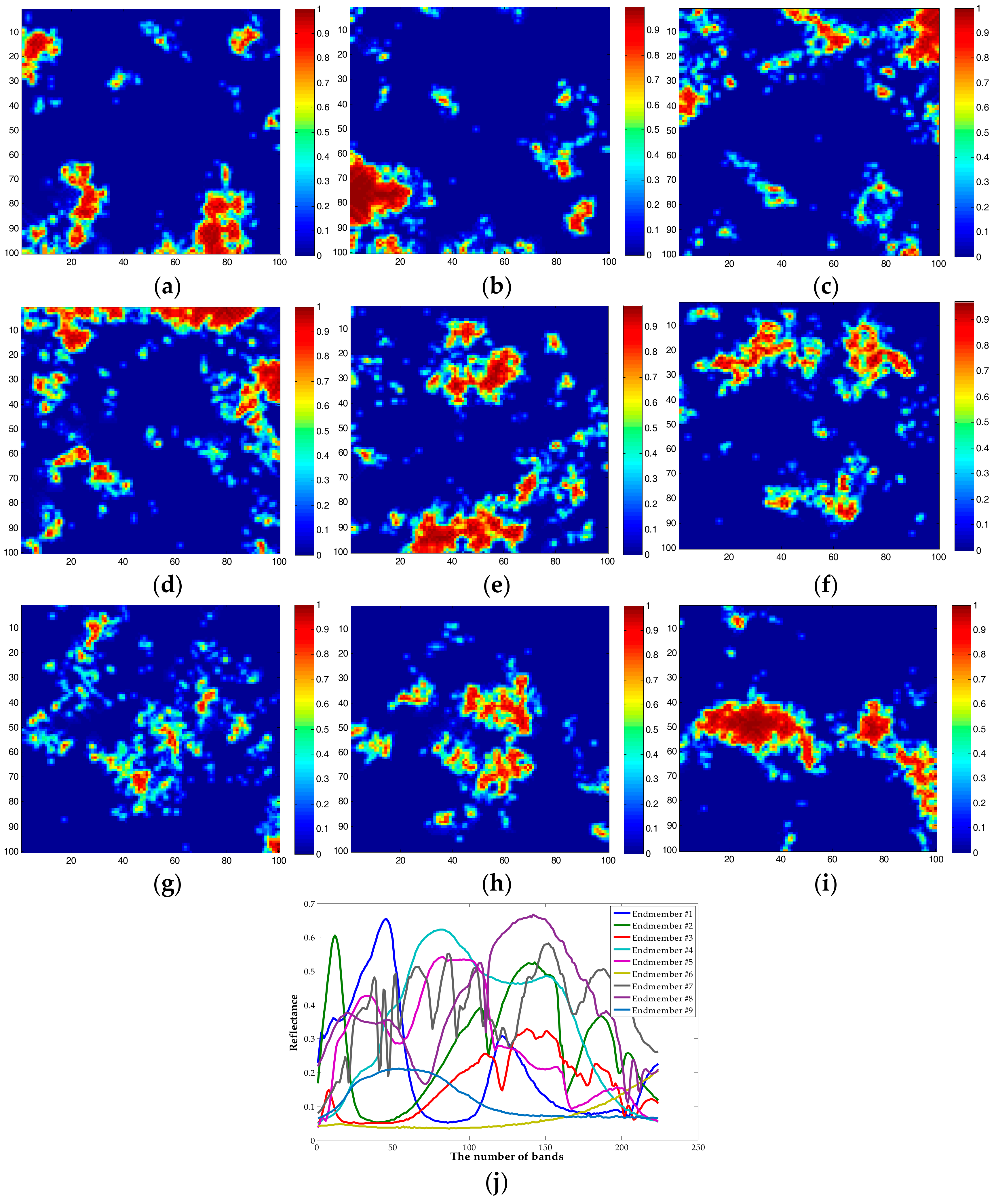
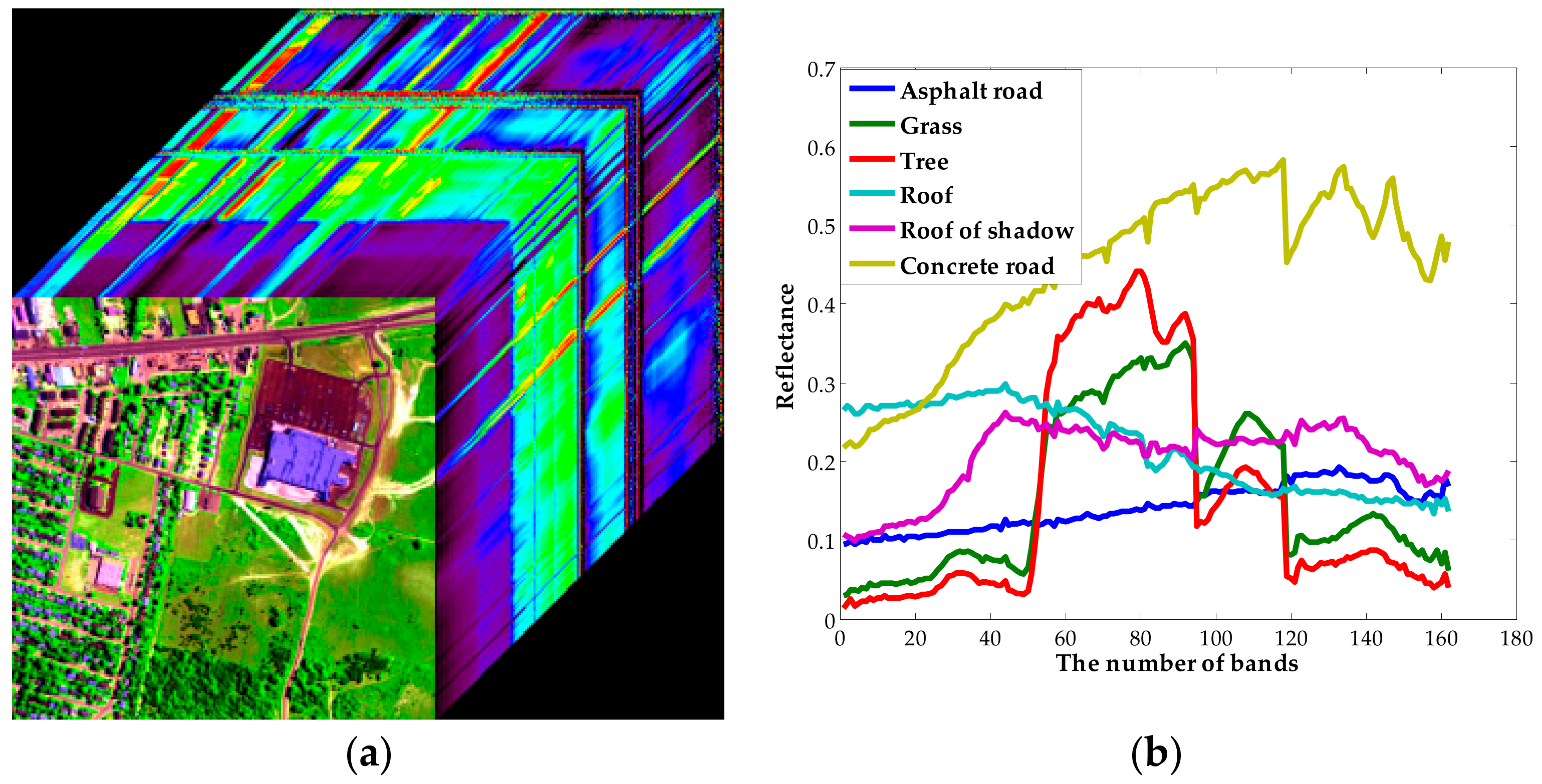
3.1. Experimental Datasets

Simulated dataset 1 (S-1): The first dataset adopted was generated following the methodology described in Reference [19], with 75 × 75 pixels and 224 bands per pixel. This dataset was generated using a linear mixture model and five randomly selected signatures as the endmembers, which were obtained from a standard spectral library, denoted as A, the famous splib06 spectral library (see http://speclab.cr.usgs.gov/spectral.lib06 for more information). In the abundance images, there were pure regions as well as mixed regions, constructed using mixtures ranging between two and five endmembers, distributed spatially in the form of distinct square regions. Figure 2a–e show the true abundances for each of the five endmembers. The background pixels were made up of a mixture of the same five endmembers, and their respective fractional abundance values were fixed as 0.1149, 0.0742, 0.2003, 0.2055, and 0.4051. These abundance values were used to analyze the effectiveness of the LARCSU algorithm. Finally, independent and identically distributed (i.i.d.) Gaussian noise was added with signal-to-noise ratio (SNR) = 30 dB. The true abundance maps of S-1 and the five selected spectral signatures are shown in Figure 2.

Simulated dataset 2 (S-2): This dataset, with an image size of 100 × 100 pixels and 224 bands, was provided by Dr. M.D. Iordache and Prof. J.M. Bioucas-Dias, and acts as a benchmark for spectral unmixing algorithms. Further details can be found in References [19,25]. Since the fractional abundances of this dataset exhibit good spatial homogeneity and can be used to simulate real remote sensing imagery, this dataset has been widely used to verify the performance of different unmixing methods. In this simulated dataset, nine spectral signatures were selected from the standard spectral library A. We then utilized a Dirichlet distribution uniformly over the probability simplex to obtain the fractional abundance maps. S-2 was also contaminated with i.i.d. Gaussian noise with SNR = 30 dB. Figure 3 illustrates the true fractional abundance maps as well as the nine spectral curves.

A real hyperspectral image (R-1) [49,50,51,52] was obtained by a Nuance NIR imaging spectrometer (650–1100 nm and a 10-nm spectral interval), with 50 × 50 pixels and 46 bands (Figure 4a), and this image was used for unmixing and to obtain fractional abundance maps. The spectral library used for this dataset was selected from the hyperspectral image obtained by the Nuance NIR imaging spectrometer as shown in Figure 4b. To make a quantitative assessment for the estimated abundance maps, a higher spatial resolution RGB image (referred to as the HR image) was also taken on the same day by a digital camera to generate the approximate true abundances maps, with 150 × 150 pixels and red, green, and blue bands, as shown in Figure 4c. These two images represent the same situation and were obtained in the same time period, but they have different spatial and spectral resolutions. To build a dataset for spectral unmixing, geometrical calibration, classification, and down-sampling were undertaken on the HR image to obtain the approximate reference abundance maps [32,50]. The specific process for the HR image was as follows. First of all, geometrical calibration was undertaken with the R-1 hyperspectral image to make sure that these two images captured exactly the same scene. Secondly, the support vector machine (SVM) algorithm was applied to the HR image to obtain the classification map. The regions of interest (ROIs) selected manually and the SVM classification map are shown in Figure 4d,e, respectively. Finally, the approximate true abundance images were obtained after down-sampling of the classification results obtained by SVM, as shown in Figure 4f. The dataset is depicted in Figure 4.

The second real hyperspectral remote sensing image used in the experiments was the Cuprite dataset (R-2), which has been widely used to validate the performance of hyperspectral unmixing algorithms. In our experiment, the portion was of 250 × 191 pixels, with 188 bands remaining after removing the bands of strong water absorption and low SNR values. In addition, the United States Geological Survey (USGS) spectral library, containing 498 standard mineral spectra, was considered as the standard spectral library A. Essential calibration was undertaken between the original hyperspectral remote sensing image and the standard spectral library. The experimental dataset is depicted in Figure 5.

The last real hyperspectral dataset (R-3) [53] was the Urban image captured by the Hyperspectral Digital Imagery Collection Experiment (HYDICE) sensor in October 1995, as shown in Figure 6a. There are 210 bands in this dataset, and the spectral and spatial resolutions are 10 nm and 2 m, respectively. The HYDICE Urban image was captured at Copperas Cove near Fort Hood, Texas, U.S., with a size of 307 × 307. According to the previous analysis, six ground objects, i.e., asphalt road, grass, tree, roof, roof shadow, and concrete road, were chosen as the endmembers and used in the spectral unmixing process in the following experiment as shown in Figure 6b. It is worth noting that there are some noisy bands with low SNR values, which were removed in our experiment.

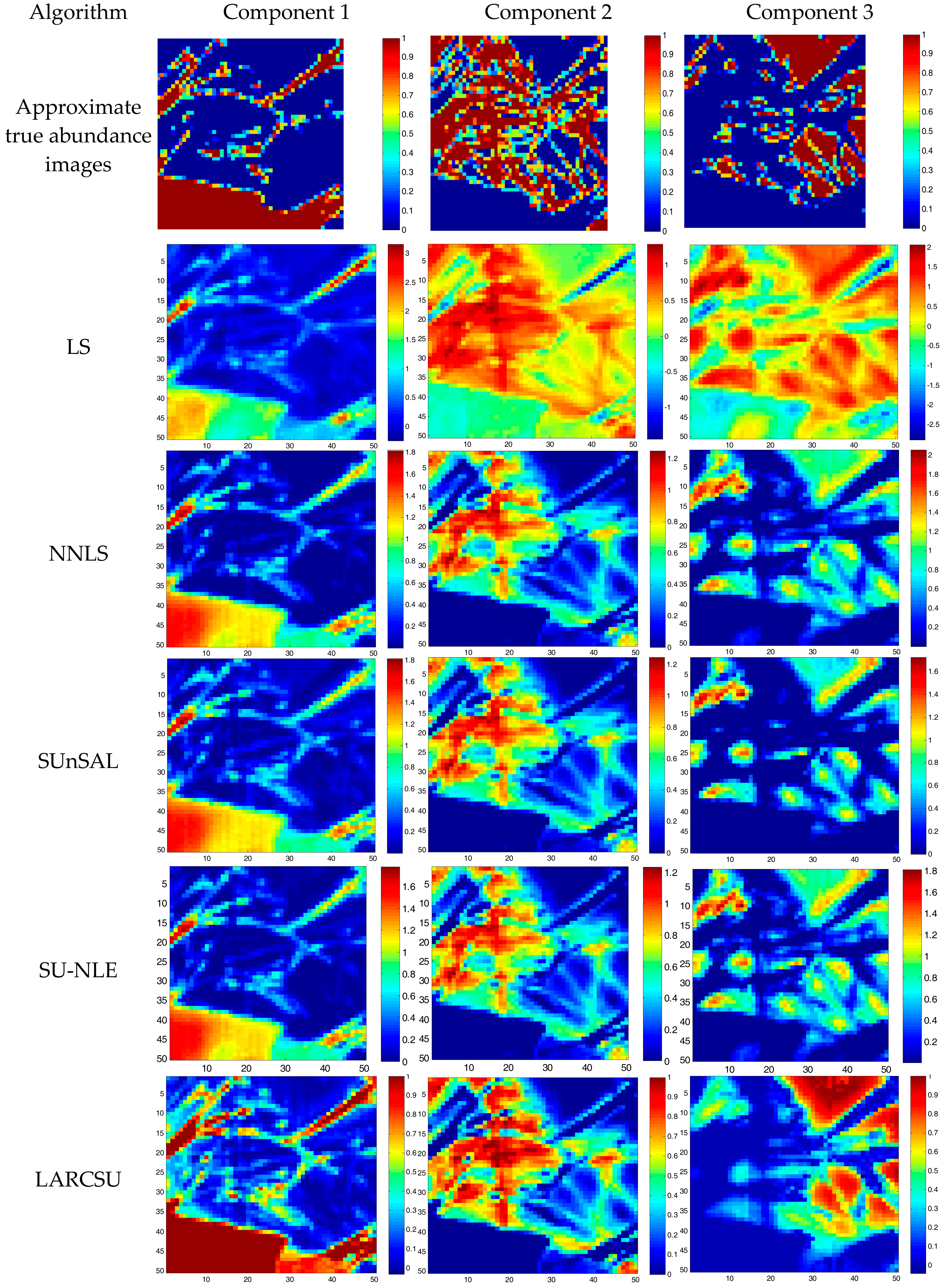
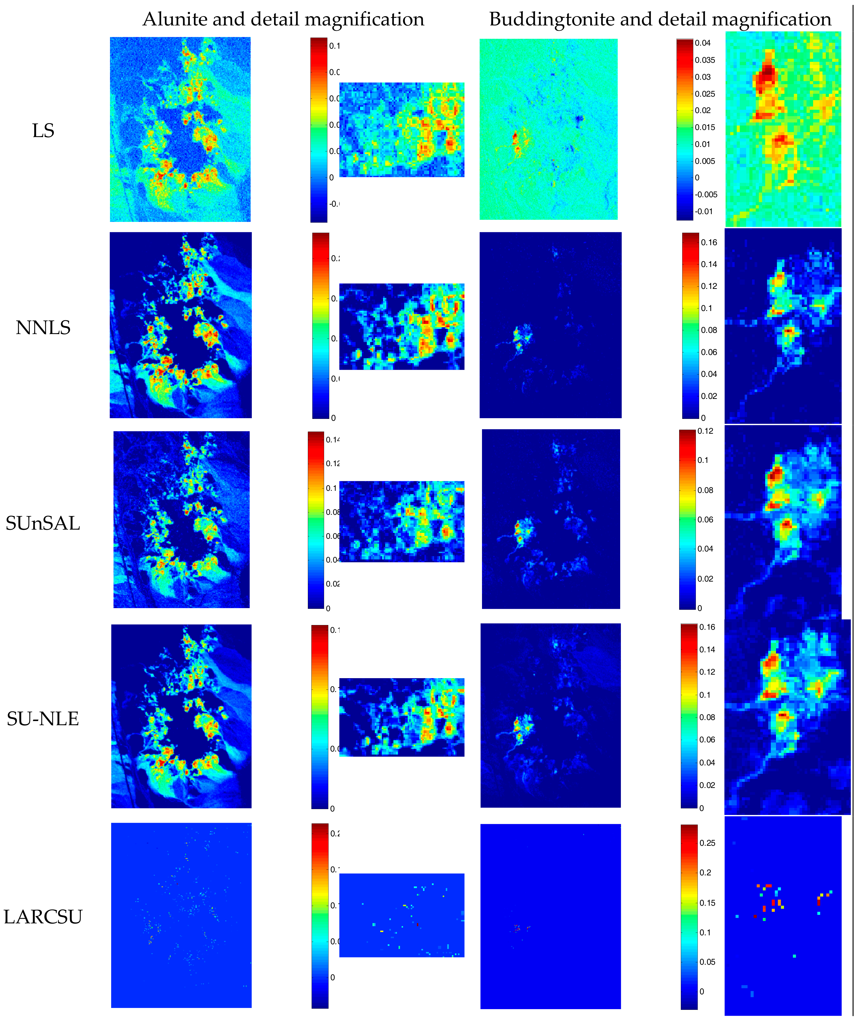
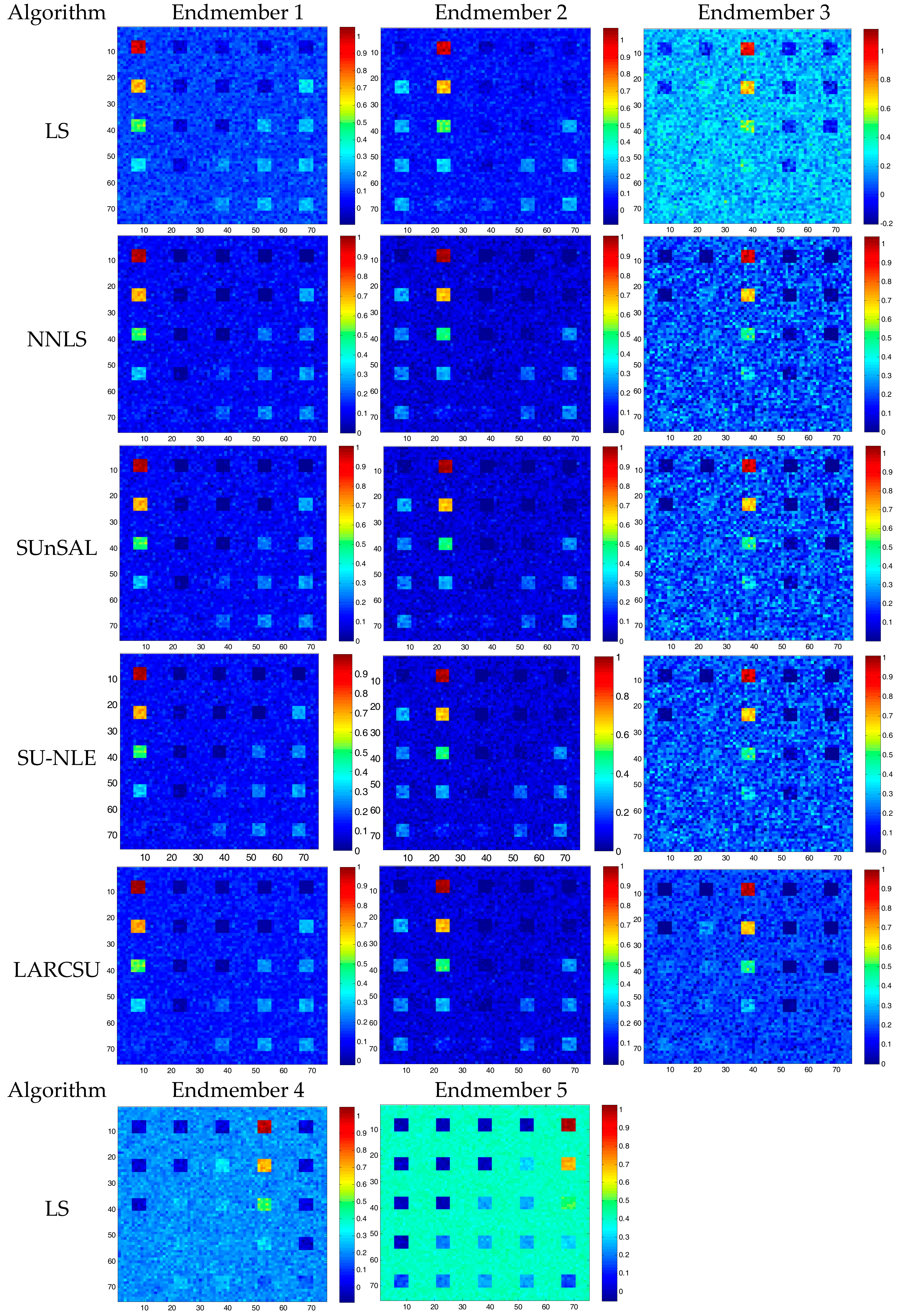
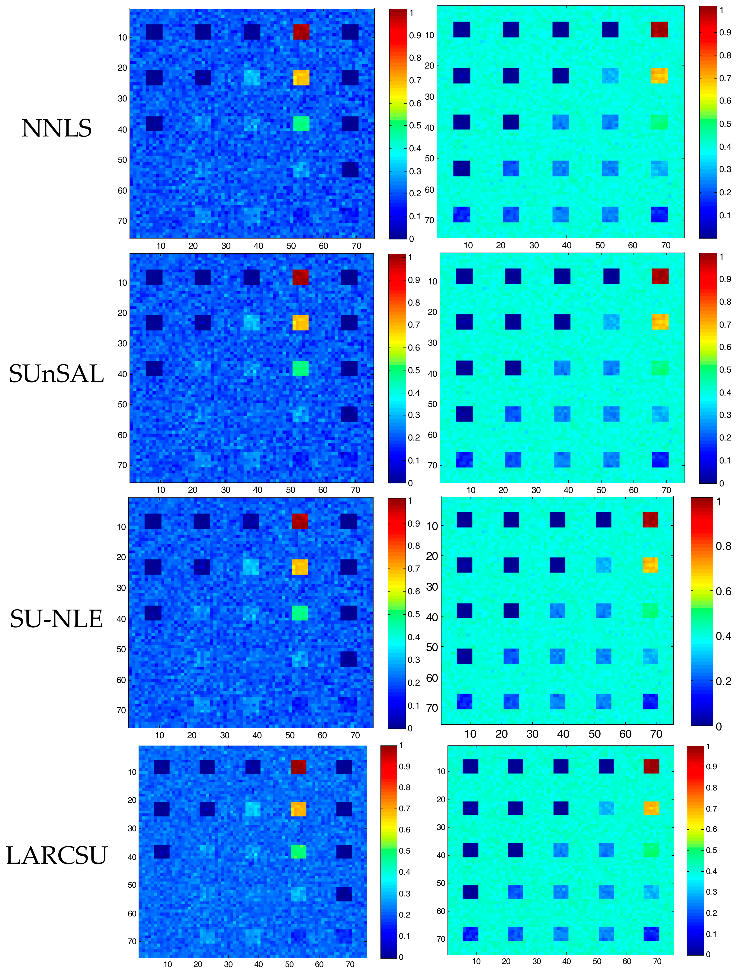
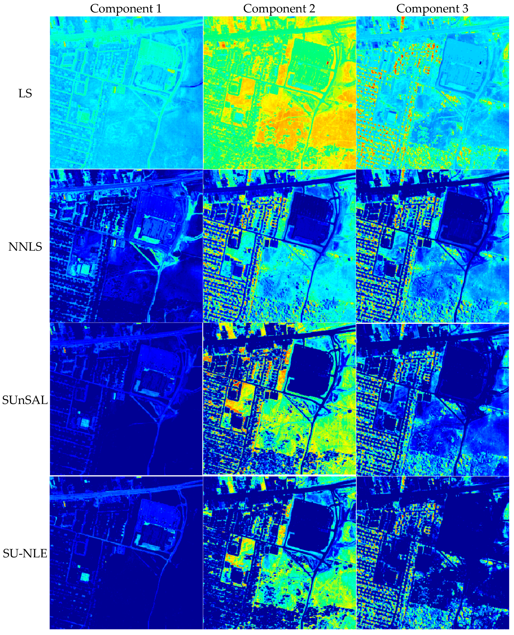
3.2. Results and Analysis

The spectral unmixing problem was solved with the above five hyperspectral datasets (S-1, S-2, R-1, R-2, and R-3) using four unmixing algorithms, i.e., LS, NNLS, SUnSAL, and LARCSU. Figure 7, Figure 8, Figure 9, Figure 10 and Figure 11 represent the fractional abundance estimations obtained for some of the representative endmember materials for each dataset. In addition,

Table 1. Performance comparison for the different methods with the five datasets.

Data	Algorithm	LS	NNLS	SUnSAL	SU-NLE	LARCSU
S-1	SRE (dB)	14.863	15.147	15.148	15.706	17.000
	RMSE	0.0435	0.0421	0.0421	0.0394	0.0340
	Time (s)	0.0156	0.5156	0.7500	13.0323	8.1563
S-2	SRE (dB)	7.528	15.710	15.886	15.88	17.000
	RMSE	0.1068	0.0416	0.0408	0.0408	0.0359
	Time (s)	0.0781	0.8281	2.7531	50.9219	20.5313
R-1	SRE (dB)	1.233	4.377	4.928	4.8570	6.366
	RMSE	0.4669	0.3251	0.3051	0.3120	0.2586
	Time (s)	0.0156	0.1406	2.9234	3.6563	2.5469
R-2	Time (s)	1.875	923.1094	1.3239 × 103	3.0393 × 104	594.7188
R-3	Time (s)	0.3281	11.7031	118.4375	928.3750	170.4219

Note: The highest signal-to-reconstructions error (SRE) and lowest root-mean-square error (RMSE) values in the table are marked in bold.

lists the SRE (dB) results achieved by the different methods with the five hyperspectral datasets.

Figure 7 and Figure 8 show the estimated abundances of the endmembers of S-1 and S-2 obtained by the different spectral unmixing algorithms. Since the five spectral unmixing algorithms do not consider the spatial information, there is no over-smoothing visible in the fractional abundance results. The most important difference among these five groups of abundance maps is the accuracy of the fitting. It can be observed that the performance of the LS unmixing method is poor in visual effect, especially for the background pixels of the estimated abundances of endmembers #1, #3, and #4 for S-1 and the estimated abundances of endmembers #3, #6, and #9 for S-2. Compared with the LS approach, the NNLS and SUnSAL algorithms display better unmixing effects on both the background and homogeneous regions. Since the i.i.d. Gaussian noise is distributed randomly and has no direct relationships with the mixed pixels, the different unmixing algorithms can do nothing but make a regression as accurately as possible. LARCSU illustrates slight advantages over the NNLS and SUnSAL methods. For example, the background of the estimated abundances of endmembers #1 and #5 of S-1 obtained by LARCSU appear much cleaner than the corresponding abundance maps obtained by NNLS and SUnSAL. LARCSU obtains similar results to the true abundance map and has a stronger noise suppression capability, especially for endmembers #2, #3, and #9 of S-2. Taking endmember #9 as an example in Figure 8, it can be observed that the outliers of the background have been effectively removed in the results of LARCSU. The rest of the wrong unmixing pixels, represented in the form of salt-and-pepper noise, could be solved with the help of spatial prior knowledge in a post-processing operation or through the use of a spatial regularization spectral unmixing method. However, in the process of mixed spectral unmixing or mixed pixel regression, the proposed LARCSU method shows some advantages over the classical approaches.

To better illustrate the process of LARCSU, the first pixel of S-1 (located at column 1, row 1) is used as an example to fully detail how LARCSU operates. For convenience, five true endmembers’ signatures are considered as different covariates D in this analysis.

Since the first pixel is a background pixel contaminated by Gaussian noise, the best estimated fractional abundances for the first pixel should be (0.1149,0.0742,0.2003,0.2055,0.4051). In the process of LARCSU, the vector of the current correlations should be computed first, after the initial setup, and the values are denoted as c, equaling (12.8160,15.4246,8.6424,18.9529,15.7332). It can be observed that the fourth endmember in the candidate endmember set has the largest correlation, and it is the first to be selected from D for the active set $\Lambda$ = {4}, where C has the current value of 18.9529. The sign flag s of the current correlation can then be obtained as 1 according to Equation (8). The key step is to compute the optimum and maximum step size of the fourth endmember’s direction. In this sub-step, the equiangular direction (${\mathbf{u}}_{\Lambda }$) should be determined first and foremost, which needs ${\Lambda }_{\Lambda }={\left(1_{\Lambda }^T{\varsigma }_{\Lambda }^{-1}{1}_{\Lambda }\right)}^{-\frac{1}{2}}=5.8848$ and ${\mathbf{\omega }}_{\Lambda }={\Lambda }_{\Lambda }{\varsigma }_{\Lambda }^{-1}{1}_{\Lambda }=0.1699$, and then ${\mathbf{u}}_{\Lambda }$ can be obtained as a 224 × 1 vector. With the candidate endmembers in D and the equiangular vector ${\mathbf{u}}_{\Lambda }$, the correlations between each variable and the equiangular vector are obtained as {2.4169,3.7035,2.3500,5.8848,4.4162}. Then, following Equation (20), we can obtain the definite β₁ (the minimum is 1.8090) from a series of potential βs = {1.8266,1.8090,2.9888,2.3280}. The first loop is then completed. Next, with the updated residual $\tilde{\mathbf{y}}=\mathbf{y}-\widehat{\mathsf{\mu }}$, the vector of the correlations c can be computed, and then the same process is repeated in cycles.

For the simple real hyperspectral image R-1, the different spectral unmixing algorithms show different unmixing performances. Considering the existence of spectral variability, the abundance sum-to-one constraint (ASC) is not enforced on all the spectral unmixing algorithms discussed in this paper, i.e., LS, NNLS, SUnSAL, and LARCSU. However, there are certain cases, in all the classical algorithms, where the abundance values obtained by LS, NNLS, and SUnSAL are greater than 1, which is against the basic law of physical constraints in spectral unmixing. As no constraints have been enforced on the LS spectral unmixing algorithm, negative abundances are widespread in the fractional abundance maps, and some abundance values even reach 300%, which is unreasonable. Differing from LS, both NNLS and SUnSAL consider the ANC, and none of their fractional abundances have negative values, with the results revealing better unmixing performances. Nevertheless, LARCSU obtains the best fractional abundance maps. As this real hyperspectral image was collected under ideal experimental conditions, apart from some systematic errors, the challenge of unmixing R-1 concerns the accuracy of the data regression. It can be observed that the results obtained by the LARCSU algorithm are significantly closer to the approximate true abundance images, which also means that LARCSU has a better data fitting ability. From Figure 9, it can also be seen that the abundance maps obtained by NNLS, SUnSAL, and SU-NLE are visually alike. Compared with these sparse unmixing methods, LARCSU is clearly superior, both in the abundance range of 0 to 1 and in the fact that the spatial homogeneity is much closer to the real distribution. In short, the LARCSU method exhibits a significant advantage in this Nuance dataset (R-1).

To validate the effectiveness of the different linear spectral unmixing algorithms, a qualitative comparison was made for alunite and buddingtonite in the Cuprite (R-2) dataset. It can be observed that the abundances obtained by LS are dense and full of noisy values. Meanwhile, the abundances obtained by NNLS, SUnSAL, and LARCSU are quite sparse, especially for LARCSU. Compared with the LS algorithm, the NNLS and SUnSAL algorithms obtain a better visual effect, and can clearly suppress the interference of the other minerals. However, unlike NNLS, LARCSU just retains the definite abundances that can best approximate the mixed pixels and wipes off the others. More details can also be found in the detail magnification in Figure 10, which can be attributed to the optimization strategy. This strategy utilizes the equiangular vector to seek the optimal regression, as well as the finite number of steps, which determines the sparsity of the abundance maps.

For the HYDICE Urban hyperspectral remote sensing image, Figure 11 shows the fractional abundance maps obtained by the different unmixing algorithms. It can be observed that LARCSU can obtain better visual unmixing results, in which the detail information is much clearer than that for the other spectral unmixing methods. Taking the middle of the homogeneous area in the Urban image as an example, the abundance values obtained by LARCSU are equal to 1 or approaching 1, seen as a red or orange color in the unmixing results in Figure 11, which is closer to the ground truth. In contrast, the results of the other unmixing approaches are mostly in yellow or cyan, which shows that the LARCSU algorithm can produce results with a better fitting quality and unmixing effect. The overall visual effect of the abundance maps in Figure 11 indicates that LARCSU is superior to the other spectral unmixing approaches.

Table 1 lists a quantitative comparison of the five spectral unmixing algorithms for simulated dataset 1 (S-1), simulated dataset 2 (S-2), and the Nuance dataset (R-1). In addition, the running times for all of the datasets (S-1, S-2, R-1, R-2, R-3) are also provided in this table. As the Cuprite dataset and the HYDICE Urban hyperspectral remote sensing image were collected by the Airborne Visible Infrared Imaging Spectrometer (AVIRIS) sensor and the HYDICE sensor, respectively, acting as real hyperspectral remote sensing imagery, there are no true or reference fractional abundance maps for the different components of these datasets. Therefore, in this paper, only the Nuance dataset is used and set as an example of a real hyperspectral dataset for the quantitative evaluation, and the abundance maps obtained from the Cuprite dataset and the HYDICE Urban image are used only for a qualitative comparison.

It can be noted that the SRE (dB) values show similar patterns to the estimated fractional abundance maps. Compared with NNLS, SUnSAL, and LARCSU, the LS method performs the worst, with the lowest SRE (dB) values of 7.528 for S-2 and 1.233 for R-1, as well as the highest RMSE values of 0.0436 for S-1, 0.1068 for S-2, and 0.4669 for R-1. Meanwhile, NNLS and SUnSAL obtain similar precisions for all three datasets, which is consistent with the abundance maps. Compared with the advanced sparse regression-based method, i.e., SU-NLE, the LARCSU algorithm shows a slightly better performance and achieves higher SRE (dB) values and the lowest RMSE values, reaching 6.366 (dB) and 0.2586, respectively, for real hyperspectral dataset R-1, which is an increase of about 30% compared with the SRE (dB) for SUnSAL. Based on the previous results and analysis, it can be inferred that LARCSU is effective in dealing with the sparse regression problem and can obtain comparable or even better regression results than the traditional ADMM-based sparse unmixing algorithms.

Table 1 also provides the running times of the different algorithms for these five datasets obtained using a PC equipped with an Intel Core i7-6700 CPU @3.4 GHz and 16 GB RAM on the MATLAB R2014a platform. From Table 1, it can be noted that the LS algorithm has the lowest time cost, and SU-NLE and LARCSU need more time to achieve a final solution. Theoretically, LARCSU should have a similar time cost to the standard CLS methods but, in practice, it takes much more time than NNLS in the experiment. Possible reasons for this may lie in the different programming tactics, mathematical calculations, etc. More research will be done to improve the efficiency of LARCSU in our future work.

4. Conclusions

In this paper, the least angle regression-based constrained sparse unmixing (LARCSU) algorithm has been proposed to further improve the sparse unmixing performance for hyperspectral remote sensing imagery. In this least angle regression model, differing from the traditional aggressive fitting idea, an equiangular vector between two predictors is utilized to seek the optimal regression steps or coefficients. In addition, unlike the ADMM-based methods that introduce some multipliers or augmented terms during their optimization procedures, LARCSU does not require any parameters in its computational process. Last but not least, theoretically, the proposed algorithm has the same order of magnitude of computational effort as the CLS-based methods.

To better illustrate the effectiveness of LARCSU, four classical traditional spectral unmixing methods were used in a comparison with two simulated hyperspectral datasets and three real hyperspectral images. Owing to the idea of the least angle regression method, LARCSU obtains better fractional abundance maps and higher precisions. In our future work, spatial regularization or spatial pre/post-processing will be considered to further enhance the LARCSU algorithm.

References

1. Tong, Q.; Xue, Y.; Zhang, L. Progress in hyperspectral remote sensing science and technology in China over the past three decades. IEEE J. Sel. Top. Appl. Earth Observ. Remote Sens. 2014, 7, 70–91. [Google Scholar] [CrossRef]
2. Plaza, A.; Benediktsson, J.A.; Boardman, J.W.; Brazile, J.; Bruzzone, L.; Camps-Valls, G.; Chanussot, J.; Fauvel, M.; Gamba, P.; Gualtieri, A.; et al. Recent advances in techniques for hyperspectral image processing. Remote Sens. Environ. 2009, 113, 110–122. [Google Scholar] [CrossRef]
3. Liu, J.; Luo, B.; Doute, S.; Chanussot, J. Exploration of planetary hyperspectral images with unsupervised spectral unmixing: A case study of planet Mars. Remote Sens. 2018, 10, 737. [Google Scholar] [CrossRef]
4. Wang, Q.; Yuan, Z.; Li, X. GETNET: A general end-to-end two-dimensional CNN framework for hyperspectral image change detection. IEEE Trans. Geosci. Remote Sens. 2018. [Google Scholar] [CrossRef]
5. Wang, Q.; Liu, S.; Chanussot, J.; Li, X. Scene classification with recurrent attention of VHR remote sensing images. IEEE Trans. Geosci. Remote Sens. 2018. [Google Scholar] [CrossRef]
6. Keshave, K.; Mustard, J.F. Spectral unmixing. IEEE Signal Process. Mag. 2002, 19, 44–57. [Google Scholar] [CrossRef]
7. Bioucas-Dias, J.M.; Plaza, A.; Dobigeon, N.; Parente, M.; Du, Q.; Gader, P.; Chanussot, J. Hyperspectral unmixing overview: Geometrical, statistical, and sparse regression-based approaches. IEEE J. Sel. Top. Appl. Earth Observ. Remote Sens. 2012, 5, 354–379. [Google Scholar] [CrossRef]
8. Ma, W.K.; Bioucas-Dias, J.M.; Tsung-Han, C.; Gillis, N.; Gader, P.; Plaza, A.; Ambikapathi, A.; Chong-Yung, C. A signal processing perspective on hyperspectral unmixing: Insights from remote sensing. IEEE Signal Process. Mag. 2014, 31, 67–81. [Google Scholar] [CrossRef]
9. Heinz, D.C.; Chang, C.-I. Fully constrained least squares linear spectral mixture analysis method for material quantification in hyperspectral imagery. IEEE Trans. Geosci. Remote Sens. 2001, 39, 529–545. [Google Scholar] [CrossRef]
10. Iordache, M.D.; Bioucas-Dias, J.M.; Plaza, A. Sparse unmixing of hyperspectral data. IEEE Trans. Geosci. Remote Sens. 2011, 49, 2014–2039. [Google Scholar] [CrossRef]
11. Shi, C.; Wang, L. Linear spatial spectral mixture model. IEEE Trans. Geosci. Remote Sens. 2016, 54, 3599–3611. [Google Scholar] [CrossRef]
12. Zhang, X.; Zhang, J.; Cheng, C.; Jiao, L.; Zhou, H. Hybrid unmixing based on adaptive region segmentation for hyperspectral imagery. IEEE Trans. Geosci. Remote Sens. 2018, 56, 3861–3875. [Google Scholar] [CrossRef]
13. Boardman, J.W.; Kruse, F.A.; Green, R.O. Mapping target signatures via partial unmixing of AVIRIS data. In Proceedings of the Fifth Annual JPL Airborne Earth Science Workshop, Pasadena, CA, USA, 23–26 January 1995. [Google Scholar]
14. Winter, M.E. N-FINDR: An algorithm for fast autonomous spectral end-member determination in hyperspectral data. Proc. SPIE 2003, 3753, 266–275. [Google Scholar]
15. Nascimento, J.M.P.; Bioucas-Dias, J.M. Vertex component analysis: A fast algorithm to unmix hyperspectral data. IEEE Trans. Geosci. Remote Sens. 2005, 43, 898–910. [Google Scholar] [CrossRef]
16. Ren, H.; Chang, C.-I. Automatic spectral target recognition in hyperspectral imagery. IEEE Trans. Aerosp. Electron. Syst. 2003, 39, 1232–1249. [Google Scholar]
17. Niroumand-Jadidi, M.; Vitti, A. Reconstruction of river boundaries at sub-pixel resolution: Estimation and spatial allocation of water fractions. ISPRS Int. J. Geo-Inf. 2017, 6, 383. [Google Scholar] [CrossRef]
18. Elmore, A.J.; Mustard, J.F.; Manning, S.J.; Lobell, D.B. Quantifying vegetation change in semiarid environments: Prevision and accuracy of spectral mixture analysis and the normalized difference vegetation index. Remote Sens. Environ. 2000, 73, 87–102. [Google Scholar] [CrossRef]
19. Iordache, M.D. A Sparse Regression Approach to Hyperspectral Unmixing. Ph. D. Thesis, School of Electrical and Computer Engineering, Ithaca, NY, USA, 2011. [Google Scholar]
20. Bruckstein, A.M.; Elad, M.; Zibulevsky, M. On the uniqueness of non-negative sparse solutions to underdetermined systems of equations. IEEE Trans. Inf. Theory 2008, 54, 4813–4820. [Google Scholar] [CrossRef]
21. Bruckstein, A.M.; Donoho, D.L.; Elad, M. From sparse solutions of systems of equations to sparse modeling of signals and images. SIAM Rev. 2009, 51, 34–81. [Google Scholar] [CrossRef]
22. Candes, E.; Tao, T. Decoding by linear programming. IEEE Trans. Inf. Theory 2005, 51, 4203–4215. [Google Scholar] [CrossRef] [Green Version]
23. Zhang, X.; Li, C.; Zhang, J.; Chen, Q.; Feng, J.; Jiao, L.; Zhou, H. Hyperspectral unmixing via low-rank representation with sparse consistency constraint and spectral library pruning. Remote Sens. 2018, 10, 339. [Google Scholar] [CrossRef]
24. Bioucas-Dias, J.M.; Figueiredo, M. Alternating direction algorithms for constrained sparse regression: Application to hyperspectral unmixing. In Proceedings of the 2nd IEEE GRSS Workshop on Hyperspectral Image and Signal Processing: Evolution in Remote Sensing (WHISPERS), Reykjavik, Iceland, 14–16 June 2010. [Google Scholar]
25. Iordache, M.D.; Bioucas-Dias, J.M.; Plaza, A. Total variation spatial regularization for sparse hyperspectral unmixing. IEEE Trans. Geosci. Remote Sens. 2012, 50, 4484–4502. [Google Scholar] [CrossRef]
26. Zhong, Y.; Feng, R.; Zhang, L. Non-local sparse unmixing for hyperspectral remote sensing imagery. IEEE J. Sel. Top. Appl. Earth Observ. Remote Sens. 2014, 7, 1889–1909. [Google Scholar] [CrossRef]
27. Salehani, Y.E.; Gazor, S.; Kim, I.-K.; Yousefi, S. L0-norm sparse hyperspectral unmixing using arctan smoothing. Remote Sens. 2016, 8, 187. [Google Scholar] [CrossRef]
28. Shi, Z.; Shi, T.; Zhou, M.; Xu, X. Collaborative sparse hyperspectral unmixing using l0 norm. IEEE Trans. Geosci. Remote Sens. 2018, 56, 5495–5508. [Google Scholar] [CrossRef]
29. Gong, M.; Li, H.; Luo, E.; Liu, J.; Liu, J. A multiobjective cooperative coevolutionary algorithm for hyperspectral sparse unmixing. IEEE Trans. Evol. Comput. 2017, 21, 234–248. [Google Scholar] [CrossRef]
30. Wang, S.; Huang, T.; Zhao, X.; Liu, G.; Cheng, Y. Double reweighted sparse regression and graph regularization for hyperspectral unmixing. Remote Sens. 2018, 10, 1046. [Google Scholar] [CrossRef]
31. Candes, E.; Tao, T. Near-optimal signal recovery from random projections: Universal encoding strategies. IEEE Trans. Inf. Theory 2006, 52, 5406–5424. [Google Scholar] [CrossRef]
32. Feng, R.; Zhong, Y.; Zhang, L. Adaptive non-local Euclidean medians sparse unmixing for hyperspectral imagery. ISPRS J. Photogramm. Remote Sens. 2014, 97, 9–24. [Google Scholar] [CrossRef]
33. Feng, R.; Zhong, Y.; Zhang, L. Adaptive spatial regularization sparse unmixing strategy based on joint MAP for hyperspectral remote sensing imagery. IEEE J. Sel. Top. Appl. Earth Observ. Remote Sens. 2016, 9, 5791–5805. [Google Scholar] [CrossRef]
34. Iordache, M.D.; Bioucas-Dias, J.M.; Plaza, A. Collaborative sparse regression for hyperspectral unmixing. IEEE Trans. Geosci. Remote Sens. 2014, 52, 341–354. [Google Scholar] [CrossRef]
35. Iordache, M.D.; Bioucas-Dias, J.M.; Plaza, A.; Somers, B. MUSIC-CSR: Hyperspectral Unmixing via Multiple Signal Classification and Collaborative Sparse Regression. IEEE Trans. Geosci. Remote Sens. 2014, 52, 4364–4382. [Google Scholar] [CrossRef] [Green Version]
36. Zhang, S.; Li, J.; Wu, Z.; Plaza, A. Spatial discontinuity-weighted sparse unmixing of hyperspectral images. IEEE Trans. Geosci. Remote Sens. 2018. [Google Scholar] [CrossRef]
37. Zhang, S.; Li, J.; Li, H.; Deng, C.; Plaza, A. Spectral-spatial weighted sparse regression for hyperspectral image unmixing. IEEE Trans. Geosci. Remote Sens. 2018, 56, 3265–3276. [Google Scholar] [CrossRef]
38. Wang, Q.; He, X.; Li, X. Locality and structure regularized low rank representation for hyperspectral image classification. IEEE Trans. Geosci. Remote Sens. 2018. [Google Scholar] [CrossRef]
39. Tibshirani, R. Regression shrinkage and selection via the Lasso. J. R. Stat. Soc. B 1996, 58, 267–288. [Google Scholar]
40. Fu, W.J. Penalized regressions: The bridge versus the Lasso. J. Comput. Graph. Stat. 1998, 7, 397–416. [Google Scholar]
41. Efron, B.; Hastie, T.; Johnstone, I.; Tibshirani, R. Least angle regression. Ann. Stat. 2004, 32, 407–451. [Google Scholar]
42. Boyd, S.; Parikh, N.; Chu, E.; Peleato, B.; Eckstein, J. Distributed Optimization and Statistical Learning via the Alternating Direction Method of Multipliers. Found. Trends Mach. Learn. 2011, 3, 1–122. [Google Scholar] [CrossRef]
43. Afonos, M.V.; Bioucas-Dias, J.M.; Figueiredo, M.A.T. An augmented Lagrangian approach to the constrained optimization formulation of imaging inverse problems. IEEE Trans. Image Process. 2011, 20, 681–695. [Google Scholar] [CrossRef] [PubMed]
44. Friedman, J. Greedy function approximation: The gradient boosting machine. Ann. Stat. 2001, 29, 1189–1232. [Google Scholar] [CrossRef]
45. Hastie, T.; Tibshirani, R.; Friedman, J. The Element of Statistical Learning: Data Mining, Inference and Prediction; Springer: New York, NY, USA, 2001. [Google Scholar]
46. Weisberg, S. Applied Linear Regression; Wiley: New York, NY, USA, 1980. [Google Scholar]
47. Li, C.; Ma, Y.; Mei, X.; Fan, F.; Huang, J.; Ma, J. Sparse unmixing of hyperspectral data with noise level estimation. Remote Sens. 2017, 9, 1166. [Google Scholar] [CrossRef]
48. Zhong, Y.; Wang, X.; Zhao, L.; Feng, R.; Zhang, L.; Xu, Y. Blind spectral unmixing based on sparse component analysis for hyperspectral remote sensing imagery. ISPRS J. Photogramm. Remote Sens. 2016, 119, 49–63. [Google Scholar] [CrossRef]
49. Feng, R.; Zhong, Y.; Wu, Y.; He, D.; Xu, X.; Zhang, L. Nonlocal total variation subpixel mapping for hyperspectral remote sensing imager. Remote Sens 2016, 8, 250. [Google Scholar] [CrossRef]
50. Xu, X.; Zhong, Y.; Zhang, L.; Zhang, H. Sub-pixel mapping based on a MAP model with multiple shifted hyperspectral imagery. IEEE J. Sel. Top. Appl. Earth Observ. Remote Sens. 2013, 6, 580–593. [Google Scholar] [CrossRef]
51. Xu, X.; Tong, X.; Plaza, A.; Zhong, Y.; Xie, H.; Zhang, L. Using linear spectral unmixing for subpixel mapping of hyperspectral imagery: A quantitative assessment. IEEE J. Sel. Top. Appl. Earth Observ. Remote Sens. 2017, 10, 1589–1600. [Google Scholar] [CrossRef]
52. Xu, X.; Tong, X.; Plaza, A.; Zhong, Y.; Xie, H.; Zhang, L. Joint sparse sub-pixel model with endmember variability for remotely sensed imagery. Remote Sens. 2017, 9, 15. [Google Scholar] [CrossRef]
53. Liu, X.; Xia, W.; Wang, B.; Zhang, L. An approach based on constrained nonnegative matrix factorization to unmix hyperspectral data. IEEE Trans. Geosci. Remote Sens. 2011, 49, 757–772. [Google Scholar] [CrossRef]
Figure 1. Schematic of least angle regression-based constrained sparse unmixing (LARCSU).
Remotesensing 10 01546 g001
Figure 2. Simulated dataset S-1. (a) Abundance map of #1. (b) Abundance map of #2. (c) Abundance map of #3. (d) Abundance map of #4. (e) Abundance map of #5. (f) The five spectra.
Remotesensing 10 01546 g002
Figure 3. Simulated dataset S-2. (a) Abundance map of #1. (b) Abundance map of #2. (c) Abundance map of #3. (d) Abundance map of #4. (e) Abundance map of #5. (f) Abundance map of #6. (g) Abundance map of #7. (h) Abundance map of #8. (i) Abundance map of #9. (j) The nine spectral curves.
Remotesensing 10 01546 g003
Figure 4. Nuance data. (a) R-1. (b) Spectral library for R-1. (c) High resolution (HR) image. (d) The regions of interest (ROIs). (e) Support vector machine (SVM) classification map. (f) Reference abundances.
Remotesensing 10 01546 g004
Figure 5. Cuprite dataset. (a) R-2. (b) Standard spectral library A.
Remotesensing 10 01546 g005
Figure 6. Hyperspectral Digital Imagery Collection Experiment (HYDICE) Urban image. (a) R-3. (b) Six endmember signatures.
Remotesensing 10 01546 g006
Figure 7. Estimated abundances of endmembers for S-1.
Remotesensing 10 01546 g007aRemotesensing 10 01546 g007b
Figure 8. Estimated abundances of the endmembers for S-2.
Remotesensing 10 01546 g008aRemotesensing 10 01546 g008bRemotesensing 10 01546 g008c
Figure 9. Estimated abundances of different components for R-1.
Remotesensing 10 01546 g009
Figure 10. Estimated abundances of alunite and buddingtonite for the Cuprite dataset.
Remotesensing 10 01546 g010
Figure 11. Estimated abundances of the different components for R-3.
Remotesensing 10 01546 g011aRemotesensing 10 01546 g011bRemotesensing 10 01546 g011c