Geocoding Error Correction for InSAR Point Clouds

Abstract

Persistent Scatterer Interferometry (PSI) is an advanced multitemporal InSAR technique that is capable of retrieving the 3D coordinates and the underlying deformation of time-coherent scatterers. Various factors degrade the localization accuracy of PSI point clouds in the geocoding process, which causes problems for interpretation of deformation results and also making it difficult for the point clouds to be compared with or integrated into data from other sensors. In this study, we employ the SAR imaging geodesy method to perform geodetic corrections on SAR timing observations and thus improve the positioning accuracy in the horizontal components. We further utilize geodetic stereo SAR to extract large number of highly precise ground control points (GCP) from SAR images, in order to compensate for the unknown height offset of the PSI point cloud. We demonstrate the applicability of the approach using TerraSAR-X high resolution spotlight images over the city of Berlin, Germany. The corrected results are compared with a reference LiDAR point cloud of Berlin, which confirms the improvement in the geocoding accuracy.

1. Introduction

In the past two decades, Interferometric Synthetic Aperture Radar (InSAR) and its multitemporal extensions have proved their ability for continuous mapping and deformation monitoring of the surface of the Earth. Among the existing InSAR approaches, Persistent Scatterer Interferometry (PSI) is nowadays considered one of the most operational techniques for wide area processing. PSI is a single-master InSAR technique that extracts phase-stable scatterers, the so-called Persistent Scatterers (PS), from a stack of SAR images and retrieves their heights along with their deformation history through the exploitation of their interferometric phase [1,2]. Its usage of multiple images and the restriction of the estimation of parameters to only PS overcomes the main limitations of InSAR, namely atmospheric disturbances and geometric and temporal decorrelation [3]. The PSI technique is highly effective in urban areas because of the availability of a high density of PS. In particular, coupling the technique with high resolution images, such as the ones from the TerraSAR-X spotlight mode, produces on average between 40,000 to 100,000 PS per square kilometer [4,5], which allows for detailed infrastructure monitoring.

Similar to other InSAR approaches, PSI is a relative technique. This means that the height and the deformation estimates of all PS are relative with respect to a reference point, which is chosen during the PSI processing [2]. For most of the cases, no information about the exact height and the stability of the reference point is available. Therefore, PSI assumes a height value extracted from the available external Digital Elevation Model (DEM) for this point and considers a height update equal to zero. Evidently, if the reference point is not stable in time and/or its true absolute height value is not equal to the corresponding DEM height, due to an erroneous DEM, the deformation and/or the height estimates of all PS will be biased. The height of PS points is an influential factor in the geocoding process. Geocoding assigns each PS to its 3D position in a geodetic reference system using the orbit parameters of the master acquisition and the estimated interferometric height [6,7,8]. Therefore, if the height estimates are biased, then the 3D coordinates of the PS will have offsets with respect to their true positions. Furthermore, the timing information of the master orbit, which is also directly involved in the geocoding process, could be erroneous due to atmospheric and geodynamic effects [9], which again hampers the localization accuracy of the PS. Assigning PS to wrong locations can lead to misrepresentation of the origin of the deformation and thus degrades the interpretation of the signal. This is in particular important for monitoring small-scale deformations in urban areas using high resolution SAR products for which the detailed structure of buildings and other objects are captured. Additionally, wrongly geocoded PSI point clouds can be neither integrated into nor compared with data from other sensors.

Several studies have been carried out in order to improve the geocoding accuracy of InSAR point clouds. In [10], the authors used an external Digital Surface Model (DSM) to evaluate a height shift between the PSI point cloud and the DSM in the vicinity of the point cloud. In [11], in addition to the usage of the DSM similar to the approach in [10], the authors installed a corner reflector in one scene and measured its position by Global Navigation Satellite System (GNSS). They radar-coded the 3D coordinates of the corner reflector and calculated a shift in range and azimuth with respect to the position of the object in the SAR image. Eventually, they corrected the entire point cloud using the three shifts: in range, azimuth and cross-range. In an alternative approach, a manual shift based on an overlay of a PSI point cloud on an ortho-rectified aerial image was used to compensate for the geocoding errors in [12]. Apart from the mentioned methods which all rely on external 2D or 3D data to correct for the errors of geocoding, two geometrical point cloud fusion approaches have been proposed in [13], which effectively compensates for the DEM error of the reference points in each of the multiaspect point clouds. The first method, which is further elaborated in [14], is based on a least squares PS matching scheme while the second approach, described in detail in [15], employs the iterative closest point (ICP) algorithm [16] to perform multiaspect point cloud matching. The first geodetic approach for reducing geocoding errors has been described in [17], in which the concepts of SAR imaging geodesy [9] and stereo SAR [18] were combined with urban SAR tomography [19] in order to absolutely localize a large number of scatterers by absolutely geolocating the manually extracted reference point.

Motivated by our work in [17] and the recently developed frameworks which automatically extract and localize Ground Control Points (GCP) from SAR images from different orbit tracks [20,21], we propose a SAR-based method for improving the geocoding accuracy of PSI point clouds. We will show that by employing SAR GCPs and applying geodetic corrections in the entire scene, one can correct for the geocoding errors as a post-processing step after the PSI processing. The applicability of the method is demonstrated in an urban area using high resolution TerraSAR-X spotlight images of Berlin, Germany. Furthermore, the results are compared with an external aerial Light Detection and Ranging (LiDAR) data, demonstrating the improvement in the geocoding accuracy of the PSI point clouds.

The remainder of the paper is organized as follows. Section 2 reviews the geocoding procedure of InSAR products and their error sources. Section 3 describes the methods used for improving the geocoding accuracy of PSI point clouds. The test site and the dataset are introduced in Section 4. The results and discussion are reported in Section 5 and the conclusions are drawn in Section 6.

2. InSAR Geocoding: Principle and Error Sources

Geocoding is performed as the final step of any InSAR processing in order to report the results in a common geodetic reference system. It is indeed a coordinate transformation from radar datum to an earth-fixed geodetic datum [7]. For each pixel in the SAR image, geocoding is carried out by iterative solving of the Doppler-Range-Ellipsoid equations to retrieve the 3D Cartesian coordinates of the target $\overrightarrow{\mathbf{T}}=\left(X_T,Y_T,Z_T\right)$ [6,8,22]:

$$∥\dot{\overrightarrow{\mathbf{S}}}\left(t_{az}\right)·\left(\overrightarrow{\mathbf{S}}\left(t_{az}\right)-\overrightarrow{\mathbf{T}}\right)∥=0,$$

(1)

$$∥\overrightarrow{\mathbf{S}}\left(t_{az}\right)-\overrightarrow{\mathbf{T}}∥-c·\frac{{\tau }_{rg}}{2}=0,$$

(2)

$$\frac{{X_T}^2}{{(a+H_T)}^2}+\frac{{Y_T}^2}{{(a+H_T)}^2}+\frac{{Z_T}^2}{{(b+H_T)}^2}-1=0,$$

(3)

where $\overrightarrow{\mathbf{S}}$ and $\dot{\overrightarrow{\mathbf{S}}}$ are the satellite state vector and its velocity vector, respectively. They are both functions of azimuth time $t_{az}$, which is the time of the closest approach, when the two-way travel time of the radar chirp ${\tau }_{rg}$ is recorded [23]. The first equation dictates the zero-Doppler condition. The second equation means that the geometric distance between $\overrightarrow{\mathbf{T}}$ and $\overrightarrow{\mathbf{S}}$ should be equal to ${\tau }_{rg}$ multiplied by the speed of light in vacuum c divided by two. The result from Equations (1) and (2) is intersected with a reference ellipsoid with semi-major axis a and semi-minor axis b and with an estimated height above the ellipsoid $H_T$ that is obtained from InSAR. The final coordinates are calculated in the Cartesian coordinate system. For convenience of interpretation, these coordinates are usually converted to the geographic coordinates ($\Phi$,$\Lambda$,H) or to the Universal Transverse Mercator (UTM) map projection (E,N,H), where $\Phi$ and $\Lambda$ are the geographic latitude and longitude while E and N denote the UTM Easting and Northing and H representing the height above the, global or local, reference ellipsoid.

Looking closely at Equations (1)–(3), the factors which influence the final position of the target after geocoding are the orbit accuracy, the radar timings ($t_{az}$, ${\tau }_{rg}$) and the estimated height of the target $H_T$. For modern SAR sensors such as TerraSAR-X, the orbit accuracy is in the centimeter regime [24,25] and therefore its effect on localization inaccuracy of targets is negligible. In the following, the other factors, namely $t_{az}$, ${\tau }_{rg}$ and $H_T$, and their error sources are briefly discussed. It is also characterized how these errors affect the final position of the target in the UTM coordinate system. It is important to note that only the errors common to all PS in a PSI point cloud, causing biased observations, are addressed here. For stochastic effects influencing individual PS, such as feature localization error depending on the Signal-to-Clutter-Ratio (SCR) of the target, the reader is referred to [22].

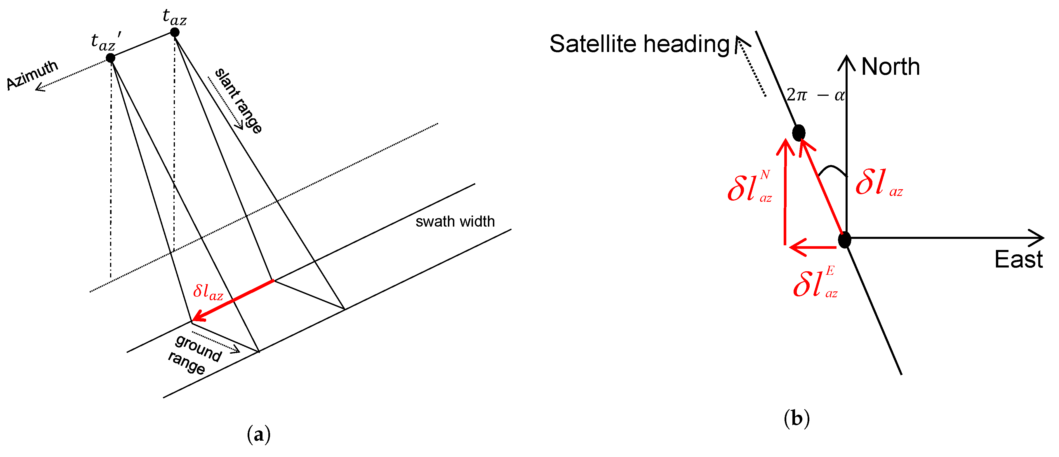
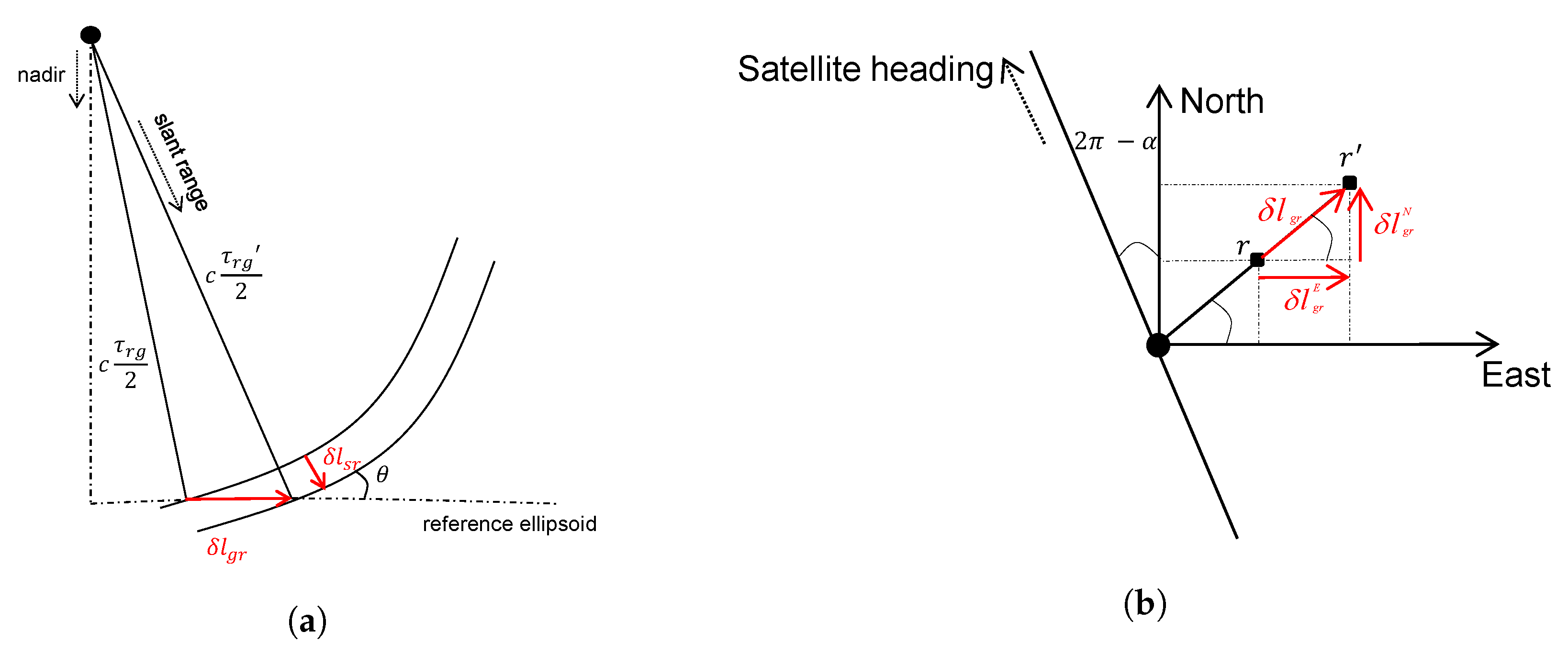
2.1. Errors in Azimuth and Range Times

The radar timings of a target can be affected by various error sources. These errors include:

• satellite dynamic effects such as incorrect annotation of $t_{az}$ in the time of radar pulse reception or incorrect annotation of ${\tau }_{rg}$ due to instrument cable delays in the satellite [9].
• propagation delays caused by the ionosphere and the troposphere, from which the latter is considered the most prominent error source on ${\tau }_{rg}$ for SAR satellites operating in X-band [7,9].
• geodynamic effects that change the position of a target on the ground, including solid earth tides, plate tectonics, ocean loading and atmospheric loading [9,18].

These errors cause biases in the timings, which are directly propagated into the final coordinates of the geocoded target through Equations (1) and (2). For $t_{az}$, the errors cause shifts only in the along track direction. If we consider a straight satellite orbit trajectory and approximate the curved Earth geometry by a rectilinear one [23], as is visualized in Figure 1a, the ground shift $\delta l_{az}$ due to an erroneous azimuth time $t_{az}^{\prime }$ is calculated in meters as:

$$\delta l_{az}=v_g\left(t_{az}^{\prime }-t_{az}\right),$$

(4)

where $t_{az}$ is the true azimuth time and $v_g$ denotes the ground-track velocity of the satellite [23]. The error affects only the horizontal geocoded coordinates and with the knowledge of the local heading angle of the satellite $\alpha$, its effect can be projected onto the local East $\delta l_{az}^E$ and North $\delta l_{az}^N$ components (see Figure 1b):

$$\begin{array}{cc}\hfill \delta l_{az}^E& =\delta l_{az}sin\alpha ,\hfill \end{array}$$

(5)

$$\begin{array}{cc}\hfill \delta l_{az}^N& =\delta l_{az}cos\alpha .\hfill \end{array}$$

(6)

Considering the near polar orbit of current SAR satellites, with heading angles close to 180° or 360°, Equations (5) and (6) show that error in $t_{az}$ mostly affects the North component of the geocoded coordinates.

Errors in ${\tau }_{rg}$ cause a delay in the received radar pulse that affects the geometrical distance between the satellite and the target in the slant range direction $\delta l_{sr}$, which leads to a displacement on the ground range $\delta l_{gr}$ depending on the the local incidence angle $\theta$ (see also Figure 2a):

$$\begin{array}{cc}\hfill \delta l_{sr}& =c\frac{\left({\tau }_{rg}^{\prime }-{\tau }_{rg}\right)}{2},\hfill \end{array}$$

(7)

$$\begin{array}{cc}\hfill \delta l_{gr}& =\frac{\delta l_{sr}}{sin\theta },\hfill \end{array}$$

(8)

where ${\tau }_{rg}$ and ${\tau }_{rg}^{\prime }$ are the true and the erroneous range time, respectively. Similar to $\delta l_{az}$, $\delta l_{gr}$ is related to the East $\delta l_{gr}^E$ and the North $\delta l_{gr}^N$ components by a projection using $\alpha$ (see also Figure 2b):

$$\begin{array}{cc}\hfill \delta l_{gr}^E& =\delta l_{gr}cos\alpha ,\hfill \end{array}$$

(9)

$$\begin{array}{cc}\hfill \delta l_{gr}^N& =-\delta l_{gr}sin\alpha .\hfill \end{array}$$

(10)

It is evident from Figure 2a and Equation (8) that $\delta l_{gr}$ becomes larger with steeper incidence angles. It is also worth mentioning that, according to Equations (9) and (10), the timing error in range manifests itself mostly in the East coordinate component.

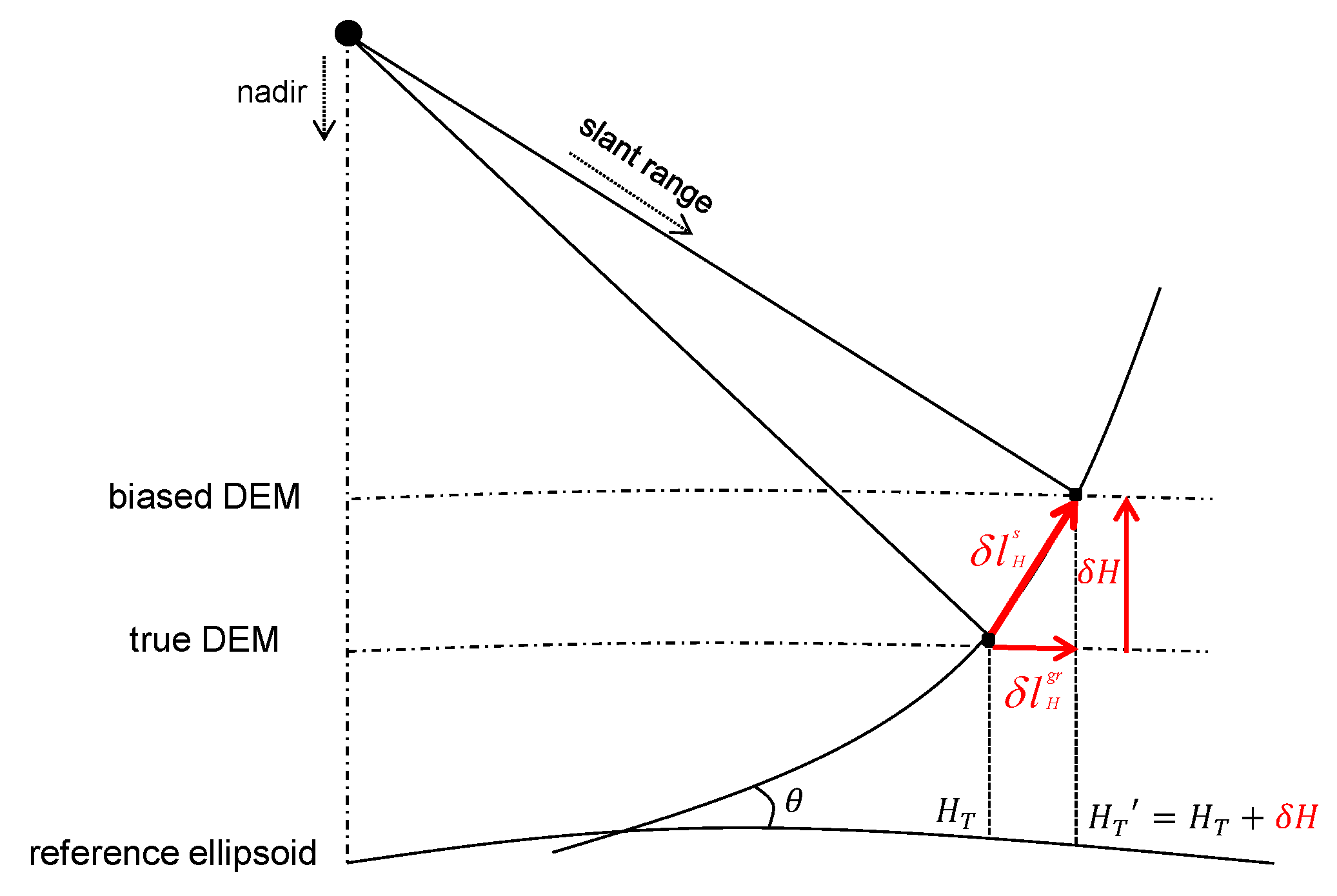
2.2. Error in the Height of PS

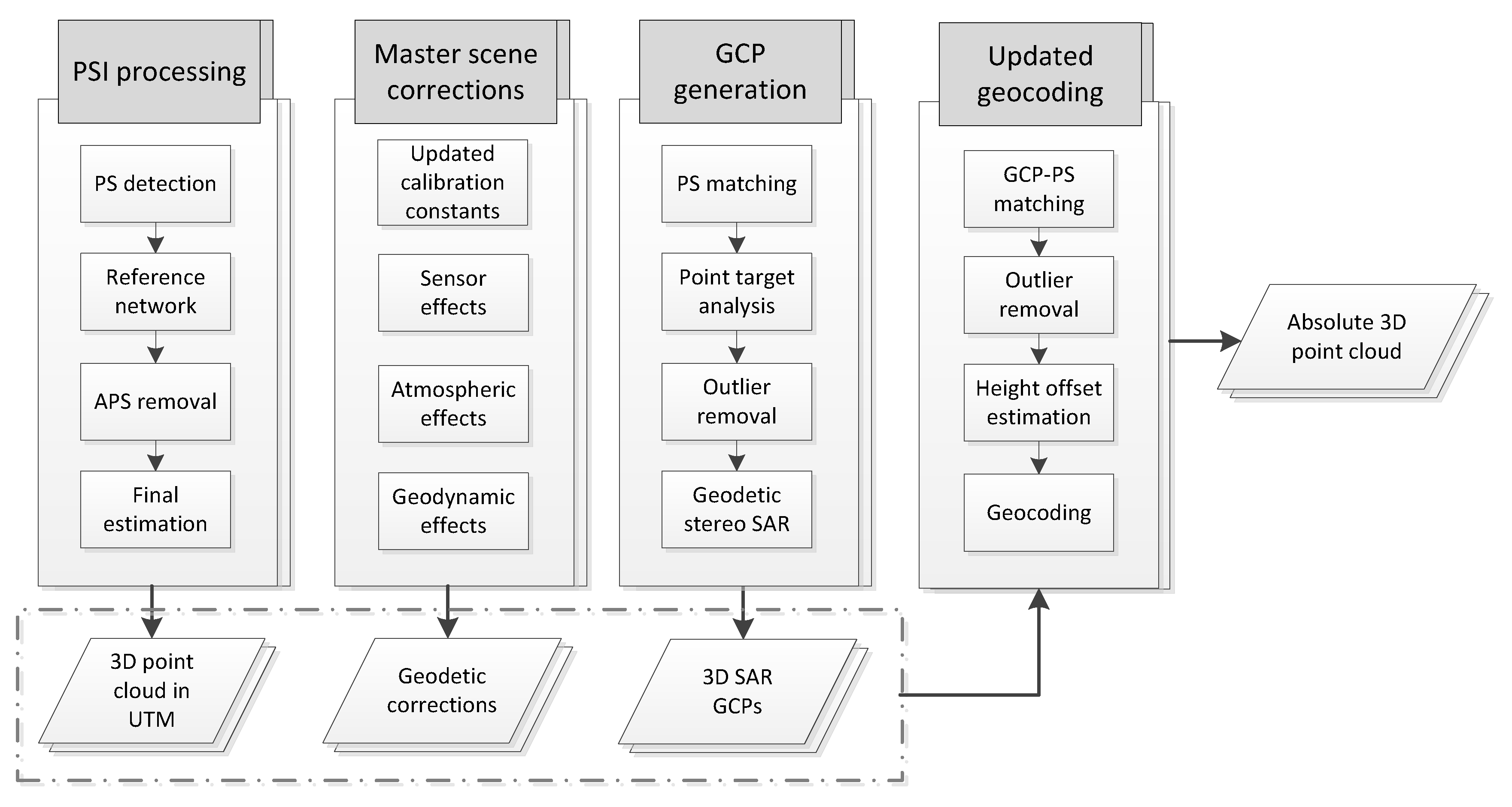
In Section 1, it was mentioned that the height estimates in InSAR approaches are defined with respect to a reference point. This implies that no DEM error is assumed for this point and its final height is equal to its corresponding DEM height. In the specific case of PSI, exploiting the differential interferograms, the DEM error for each PS is estimated relative to the reference point and at a later step before geocoding, the DEM height of each PS is added to its DEM error to obtain the final PS height denoted by $H_T^{\prime }$. It is obvious that the final absolute height accuracy of all PS depends on the DEM error of the reference point, which is an overall unknown offset. This height error $\delta H=H_T^{\prime }-H_T$ is constant for all PS and has a significant effect on final geocoded coordinates both in the horizontal and in the vertical components, as can be seen in Figure 3. The variable $\delta H$ causes a horizontal shift in the ground range $\delta l_H^{gr}$ as:

$$\delta l_H^{gr}=\frac{\delta H}{tan\theta }.$$

(11)

Similar to the error in range timing (see Equations (9) and (10)), $\delta l_H^{gr}$ can be projected onto the East and the North components by knowledge of $\alpha$.

3. Methodology

The error sources and their impact on the localization of InSAR point clouds have been addressed in Section 2. In this section, we present our proposed framework for the estimation and removal of the aforementioned biases, which leads to an improvement of the overall geocoding accuracy of PSI point clouds. The method is divided into four parts, which are briefly explained in the following and are depicted in Figure 4. Each processing step is carried out independently and produces an intermediary result, which is shown as a parallelogram in Figure 4. The double shapes indicate that two or more SAR image stacks are involved in each processing. The intermediary results, gathered in the dashed gray rectangle, are the input for the fourth step, updated geocoding, which produces the final absolute 3D PSI point clouds. Please note that the input for our approach includes a minimum of two SAR image stacks acquired from different viewing geometries i.e., from separate orbits. This is required for the extraction of highly precise GCPs. Apart from the methodology description, the procedure to compare the geocoded PSI point clouds with external LiDAR data is also explained in this section.

3.1. PSI Processing

A concise description of the PSI technique has been given in Section 1. The major steps of the processing chain are outlined in Figure 4. The output of the PSI processing are the geocoded 3D UTM coordinates of PS and their displacement parameters. For details about the theory of the method and its processing sequence, the interested reader is referred to [1,2].

3.2. Master Scene Corrections

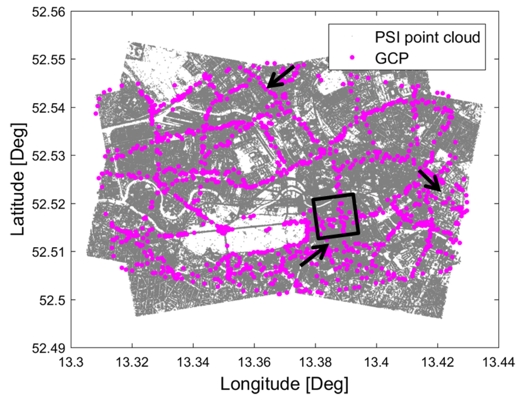
Geocoding is commonly carried out based on the orbit and the timing information of the master SAR image. In order to provide unbiased $t_{az}$ and ${\tau }_{rg}$, the errors stated in Section 2.1 are mitigated by the SAR imaging geodesy approach [9,26,27,28,29]. The ionospheric path delay is corrected on base of the global Total Electron Content (TEC) maps that use the single layer model [30] for ionosphere. Using the orbit information of the SAR satellite, the point at which the line of sight of the satellite passes through the ionospheric layer to the point of interest is analytically localized. The zenith TEC value is then determined at the location of the aforementioned point through spatial and temporal interpolation of the TEC maps [27,31,32]. Subsequently, the vertical TEC value at the point is projected onto the line of sight of the SAR satellite using a proper mapping function [31]. The path delay caused by troposphere is computed through the 4D integration of numerical weather data from European Centre for Medium-Range Weather Forecasts (ECMWF). The method extracts the dataset from a local database, converts it to a conventional geographic coordinate system, performs a 3D interpolation for defined integration points and eventually integrates the refractivity index along the integration path in the slant-range direction from the point of interest to the satellite [15,26]. The geodynamic effects are removed based on the state-of-the-art models according to the International Earth Rotation and Reference Systems Service (IERS) guidelines [33]. The effects are reported in the horizontal and the radial coordinate components, which are transformed to the radar timing coordinate system [9]. The coordinate transformation residuals between object and sensor coordinate systems are compensated for by taking into account the plate tectonics effect and referring the observation to a reference epoch [26]. Finally, the geometric calibration constants in range and azimuth are updated based on the most recent studies concerning long-term corner reflector experiments [34]. For this purpose, all the aforementioned effects are initially mitigated using the described methods and then the median of offsets between the expected position of the corner reflector, surveyed with GNSS, and its corresponding position in a time series of SAR images is considered as new re-calibration constants [34]. All of the mentioned corrections are computed for a coarse grid and are further interpolated for targets inside the grid [35]. The corrections are subtracted from the annotated SAR measurements to achieve absolute $t_{az}$ and ${\tau }_{rg}$. For more information regarding SAR imaging geodesy and its operational implementation, the reader is referred to [9,26,34,35].

3.3. GCP Generation

The first step regarding the GCP generation is the correct detection of identical PS from multiaspect SAR images. After the calculation of corrections (see Section 3.2), for each individual Single Look Complex (SLC) image, bright point-like targets are extracted through the spatial analysis of their SCR. It is important to mention that for the extraction of GCP candidates, PS from the previously generated PSI point clouds can be used as well, as has been shown in [21]. However, since our aim is to show the flexibility of the geocoding error correction approach, independent from which GCP candidate detection method is used, we use a completely separate processing chain from PSI processing in order to extract GCPs [20]. After the GCP candidate detection, target radar coordinates are geocoded using an external DEM and a point-matching scheme is carried out to find the correspondence of each target in other SLCs with different viewing geometries [20]. The method then extracts the precise timing information of each point target in all SLCs through Point Target Analysis (PTA) [23]. Finally, identical PS timings from multiaspect data are combined using stereo SAR to estimate the absolute 3D coordinates of each PS [18]. The individual steps are also depicted in the workflow in Figure 4, where the last step, called geodetic stereo SAR, refers to the combination of the SAR imaging geodesy and the stereo SAR methods. The output of this part is several thousands of GCPs with absolute 3D coordinates.

A further filtering of the GCPs is carried out based on their posterior coordinate standard deviations, which are also the output of the GCP extraction framework. The threshold for this filtering is chosen based on our previous studies dealing with the stereo localization of natural PS [18,21]. As a final refinement, we filter the GCPs based on their closeness to the road network data of the scene, which can be freely accessed either from OpenStreetMap [36] or from country-specific geo-portals as demonstrated in [21]. The reason for the latter filtering is that the most reliable GCP targets are the ones that can be easily recognized from cross-heading geometries. In urban areas, these targets include lamp poles and traffic signs, which are commonly found close to streets and roads. For different approaches of SAR GCP generation using high resolution SAR data, the interested reader is recommended to consult [20,21].

3.4. Height Offset Estimation and Updated Geocoding

The objective of this processing step is to calibrate the height coordinates of the PS in PSI point clouds by using the generated SAR-based GCPs. In order to estimate the DEM error of the reference point of each PSI point cloud, the first step is to find for each GCP its corresponding point in the PSI point cloud since different processing chains were used for PSI processing and GCP generation (see Section 3.3). To this end, we radar-code the GCP coordinates onto the master scenes of each SAR image stack taking into account the full geodetic corrections. We then select the nearest neighbor of the GCP in the PS point cloud that has an Amplitude Dispersion Index (ADI) lower than a threshold [1]. In this way, we can correspond each GCP to its closest PS that most likely represents the base of lamp poles or traffic signs. However, this approach is highly prone to detecting wrong correspondences since the ADI of the lamp pole might be higher than the predefined threshold. To overcome this limitation, we further refine the GCP-PS correspondence detection as follows:

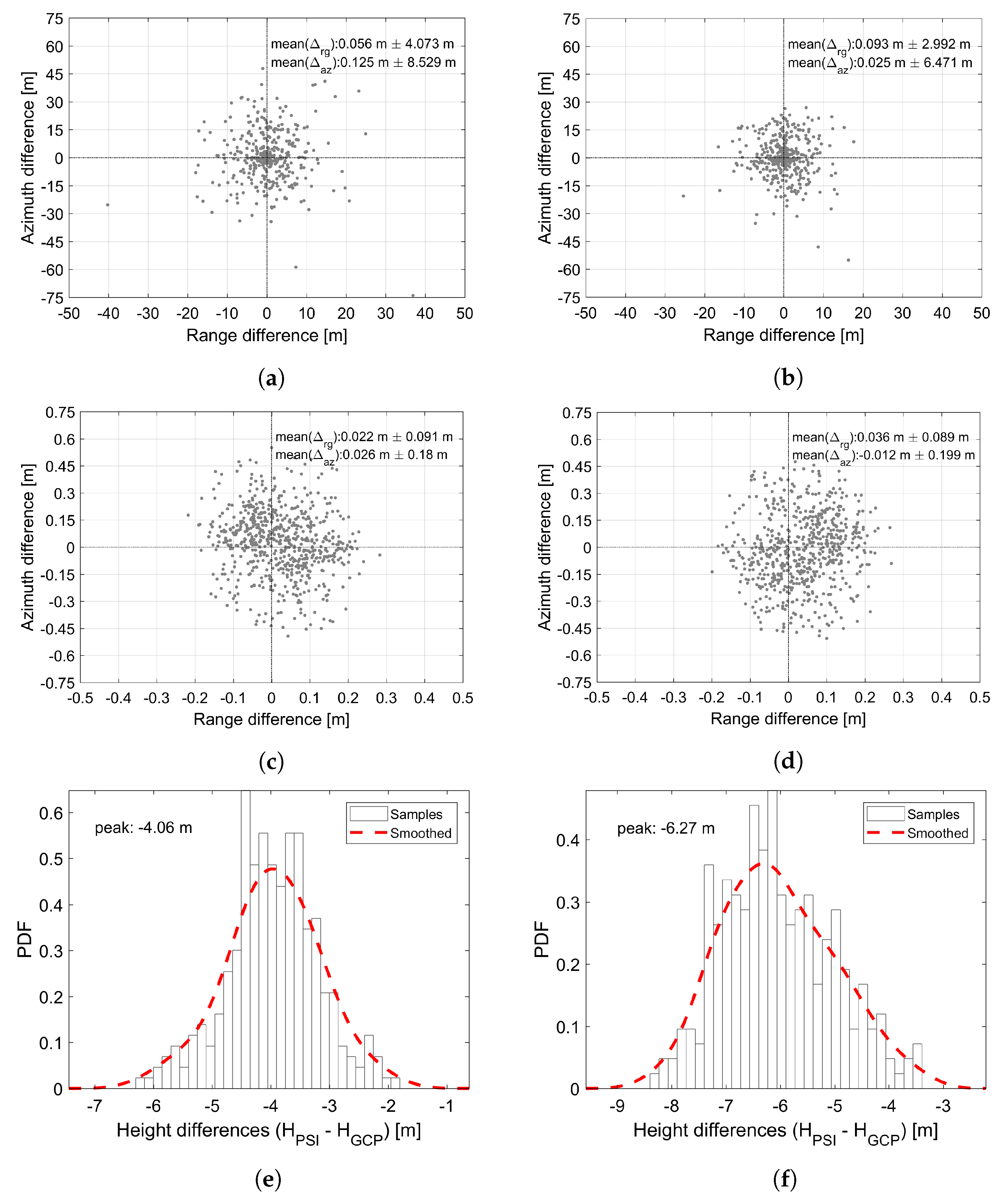
• Coordinate differences are calculated in range and azimuth of the GCPs and their assumed corresponding bright point in the PSI point cloud.
• Points with coordinate differences larger than two times the standard deviation of differences (2$\sigma$ rule) are discarded first in range and then in azimuth.

Note that, due to the probable existence of outliers, the standard deviation of coordinate differences is robustly estimated using the Median Absolute Deviation (MAD) measure [37]. The reason for the strict measure in the second step is that the geodetic and the propagation errors on range and azimuth of a TerraSAR-X spotlight scene usually vary within centimeter and millimeter regimes, respectively. Therefore, large coordinate difference variations show that the wrong correspondence between the GCP and the bright point has been detected and lead to discarding the candidate.

After the correspondence detection has been refined, we need to robustly estimate a single height offset among GCP heights and their corresponding PS heights. Initially, the GCP-PS ellipsoidal height differences are calculated. The dispersion of height differences is estimated using MAD. Furthermore, large height difference observations are discarded based on the $2\sigma$ rule, while the distance of each observation is evaluated with respect to the median of the differences to ensure robustness [37]. Subsequently, the outlier-free height difference histogram is formed. The peak of the smoothed histogram is detected as the mode of height differences, which is the approximate estimate of the DEM error of the reference point.

The estimated height offset is subtracted from the ellipsoidal heights of the geocoded PSI point cloud to obtain correct absolute heights. At the final step, the corrected heights as well as the corrected range and azimuth timings (see Section 3.2) are used for an updated geocoding using Equations (1)–(3). The result is the corrected geocoded 3D PSI point cloud in either Cartesian or UTM coordinate system.

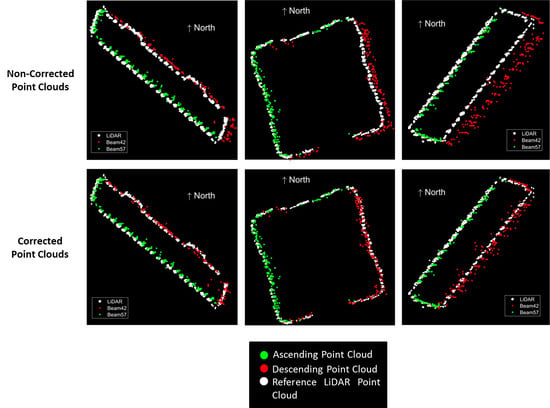
3.5. Cross-Comparison with LiDAR

In order to check the overall localization accuracy of PSI point clouds after correcting for the geocoding errors, we carry out qualitative and quantitative horizontal and vertical analyses with respect to a reference LiDAR data. Since data from LiDAR are acquired with a nadir-looking geometry in contrast to the slant-viewing geometry of SAR sensors, we should make the data from both sensors as compatible as possible. To this end, we first extract the PS originated from façade of buildings using an approximate approach proposed in [14]. For each PS, a neighborhood is selected in the horizontal plane within which the variance of PS heights is evaluated. If the variance is higher than a threshold, the point is considered to be a façade PS [14]. A similar approach is carried out to extract the 2D building footprints from the LiDAR point cloud. After the separation of façade and non-façade points in the UTM coordinate system, the localization accuracy analysis is carried out as follows:

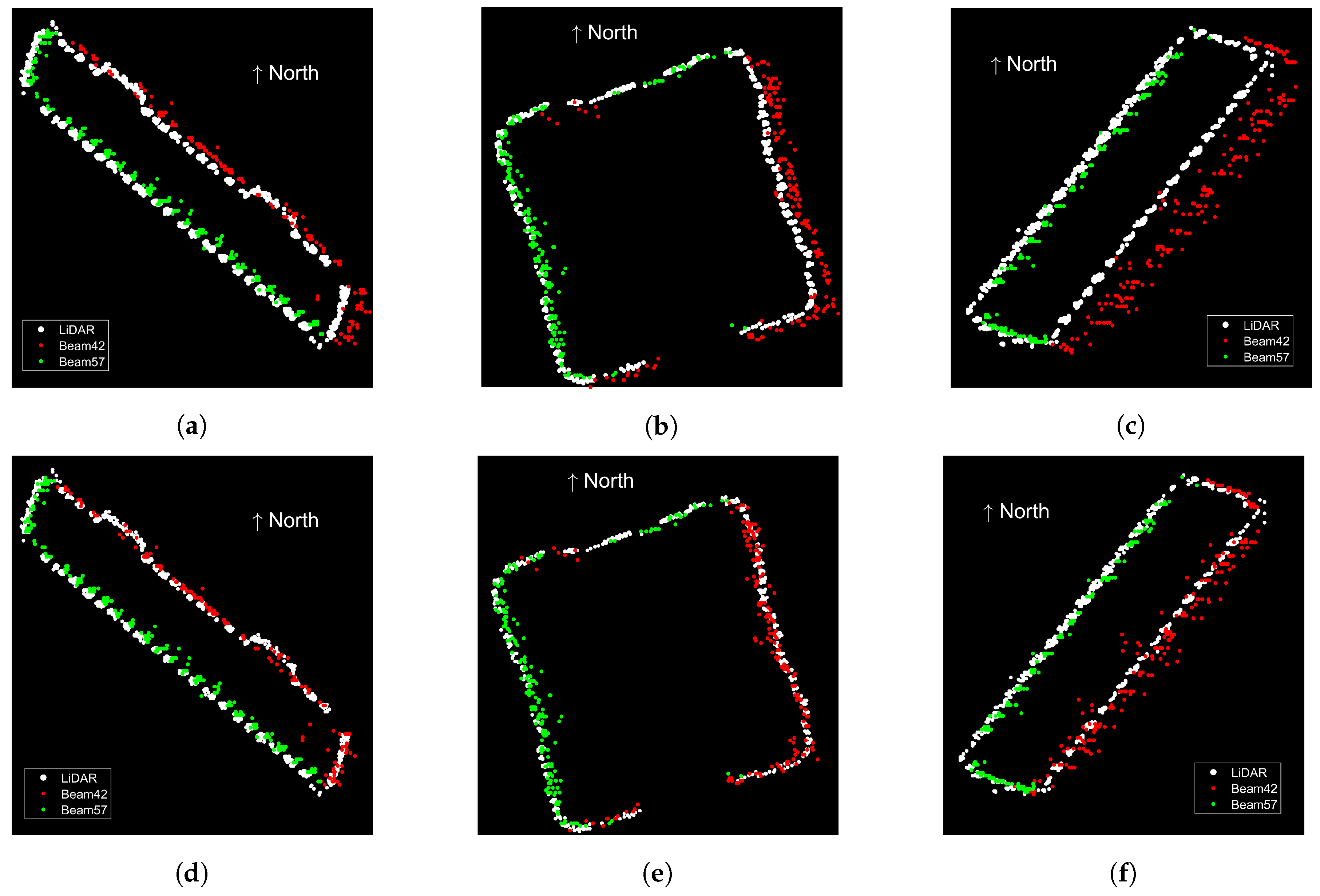
• 2D horizontal accuracy: For a number of test sites, a line is robustly fitted to each side of the building footprint in the LiDAR point cloud in the East–North plane. The mean distance of the façade PS in the PSI point clouds are evaluated with respect to the corresponding footprint line in the LiDAR data. The average of all the deviations for corrected and non-corrected PSI point clouds are separately calculated, which demonstrates the closeness of each point cloud to the reference LiDAR data.
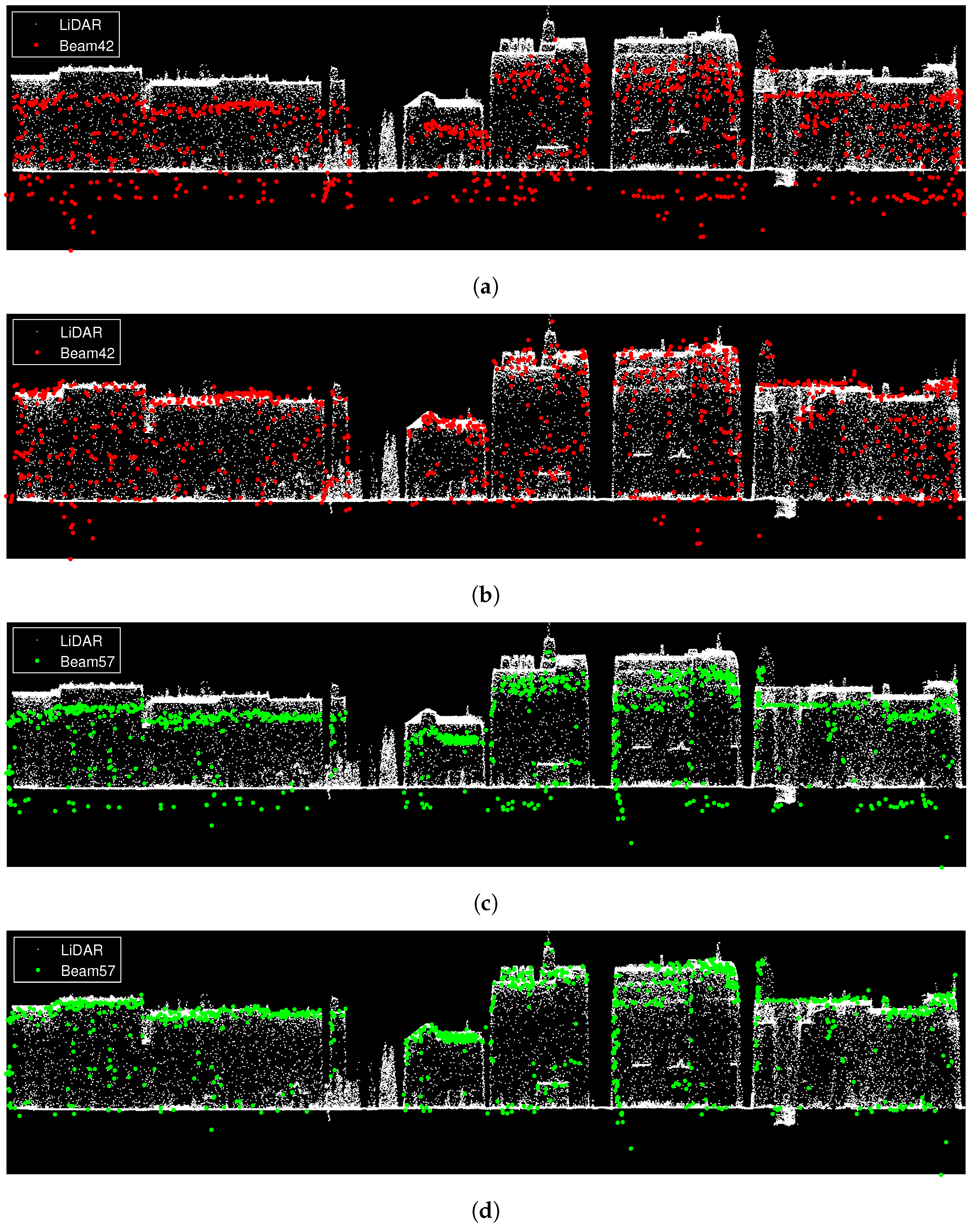
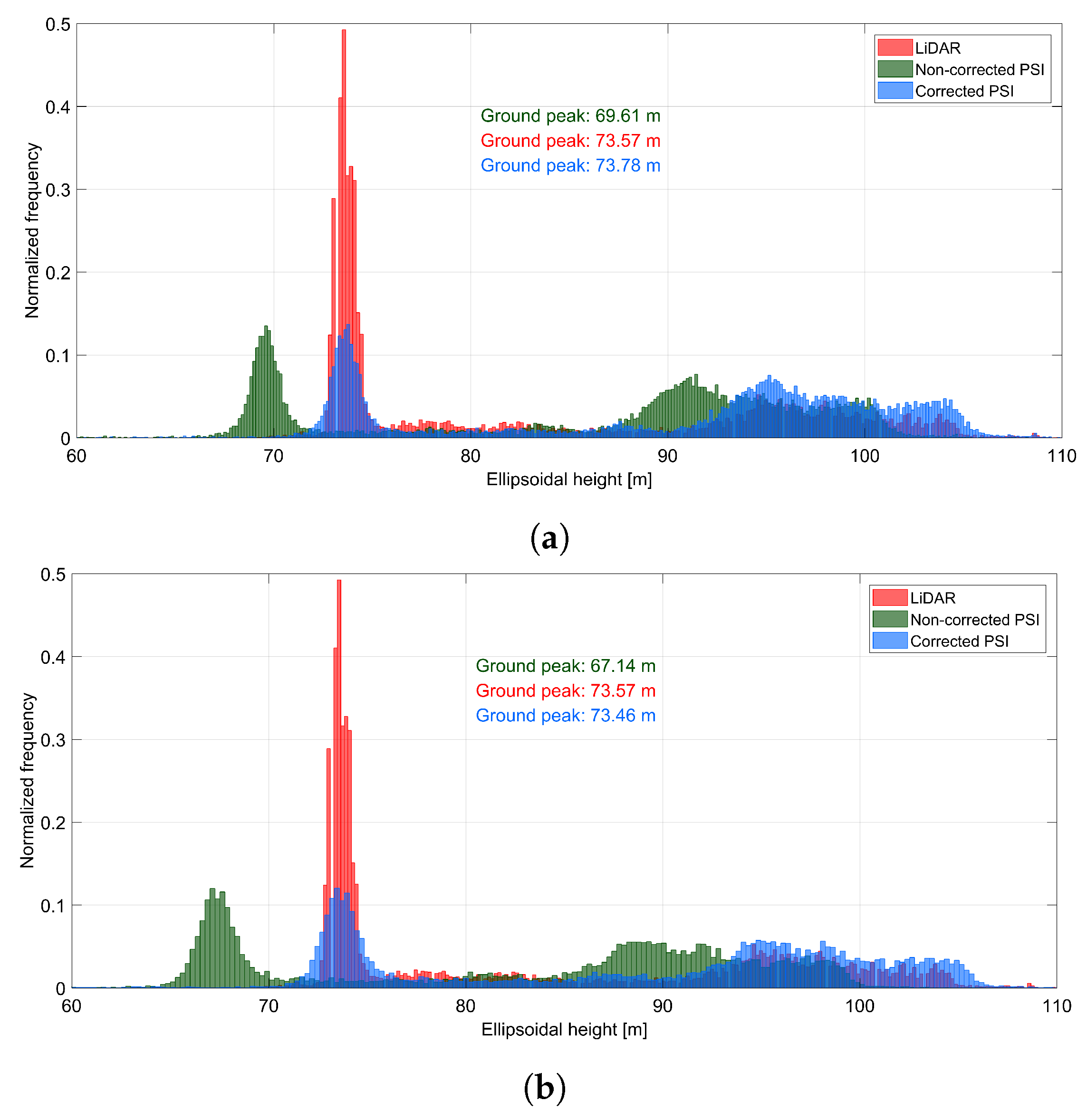
• 1D vertical accuracy: For an identical area in the LiDAR data and both corrected and non-corrected PSI point clouds, the façade points are excluded. Then for each of the three point clouds, ellipsoidal height histograms are formed containing two peaks which respectively represent ground and building roofs from the selected test site. The difference between the height values for which the ground peaks, in the PSI point cloud and in the LiDAR point cloud occur, indicates the vertical accuracy.

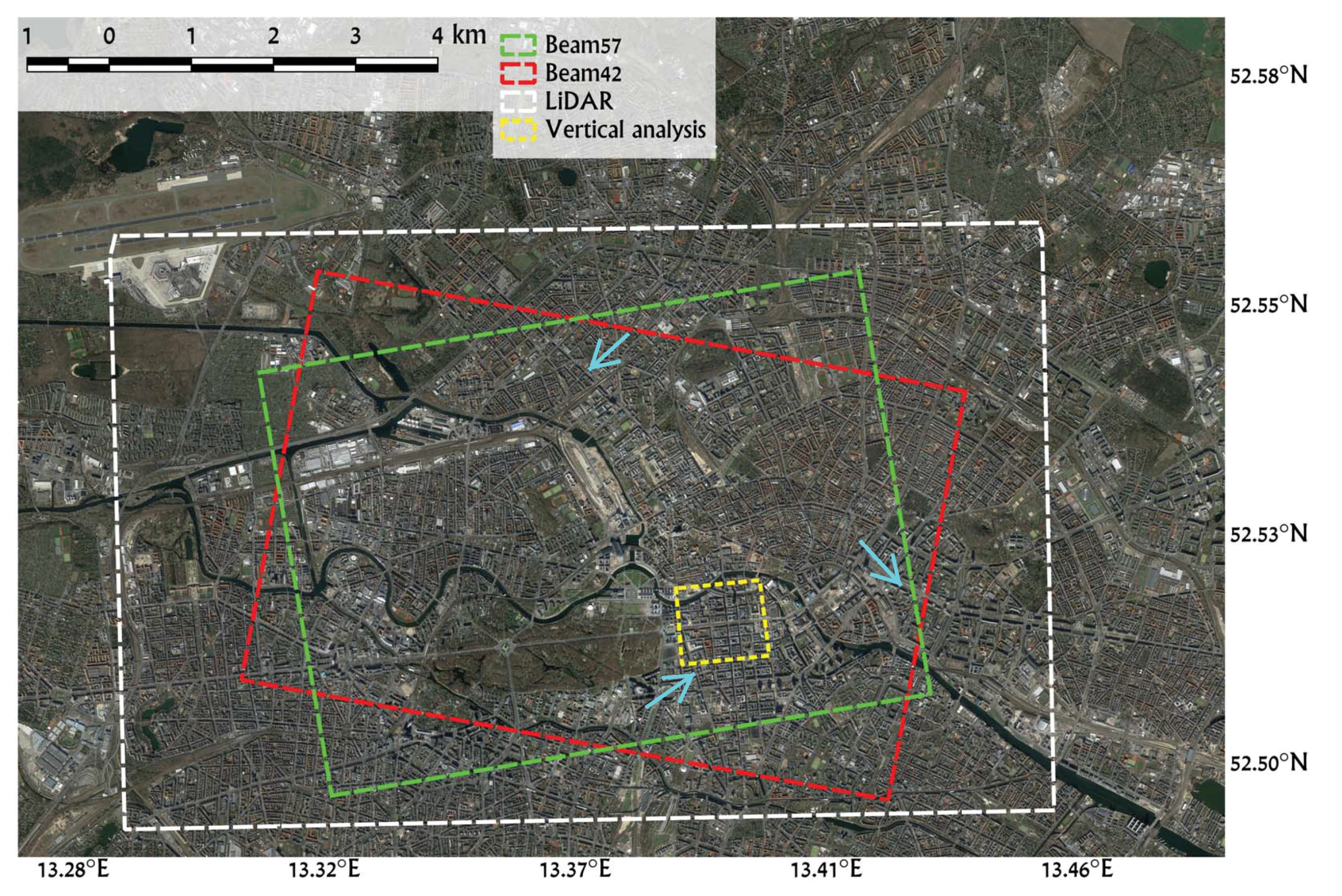
4. Area of Interest and Data Set

The investigated test site includes the central urban area of Berlin located in northeastern Germany. Our data set includes two stacks of TerraSAR-X high-resolution spotlight products with nominal spatial resolution of 1.1 m in azimuth and 0.6 m in range. The total number of images is 214, which cover a period of approximately five years from April 2010 to March 2015. In terms of viewing geometry, one stack is acquired from a descending orbit track and the other one from an ascending orbit with approximate incidence angles of 36° and 42°, respectively. In addition to the SAR data, an aerial LiDAR point cloud with a 3D accuracy in the decimeter regime is available, for which the acquisition period is from January to March 2009. The LiDAR data is used as reference to check the absolute 3D localization accuracy of PSI point clouds. The acquisition parameters of each SAR image stack are reported in

Table 1. Acquisition parameters of stacks of SAR images in Berlin.

Beam Nr.	Center θ (Degree)	Average α (Degree)	Orbit Direction	Area (km2)	Polarization	Nr. of Images
42	36.1	350.3	descending	40.94	VV	107
57	41.9	190.6	ascending	42.52	VV	107

. The mean scene coverage of the SAR images, the extent of the LiDAR data and the test sites used for vertical and horizontal accuracy analysis are marked in Figure 5.

5. Results and Discussion

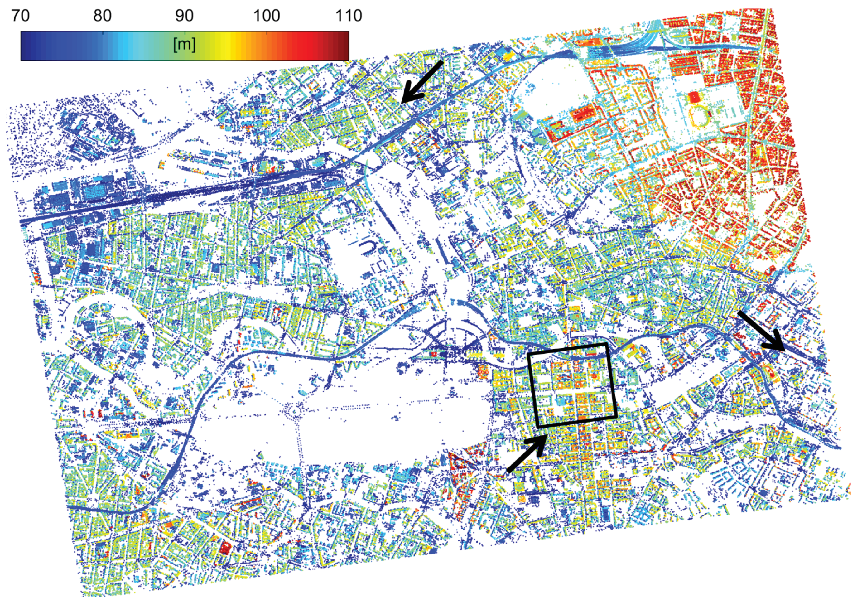
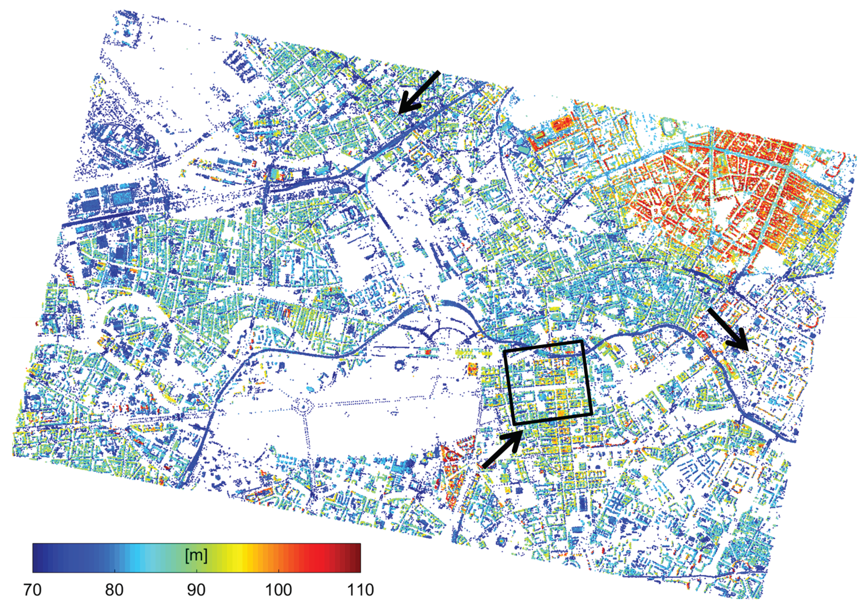
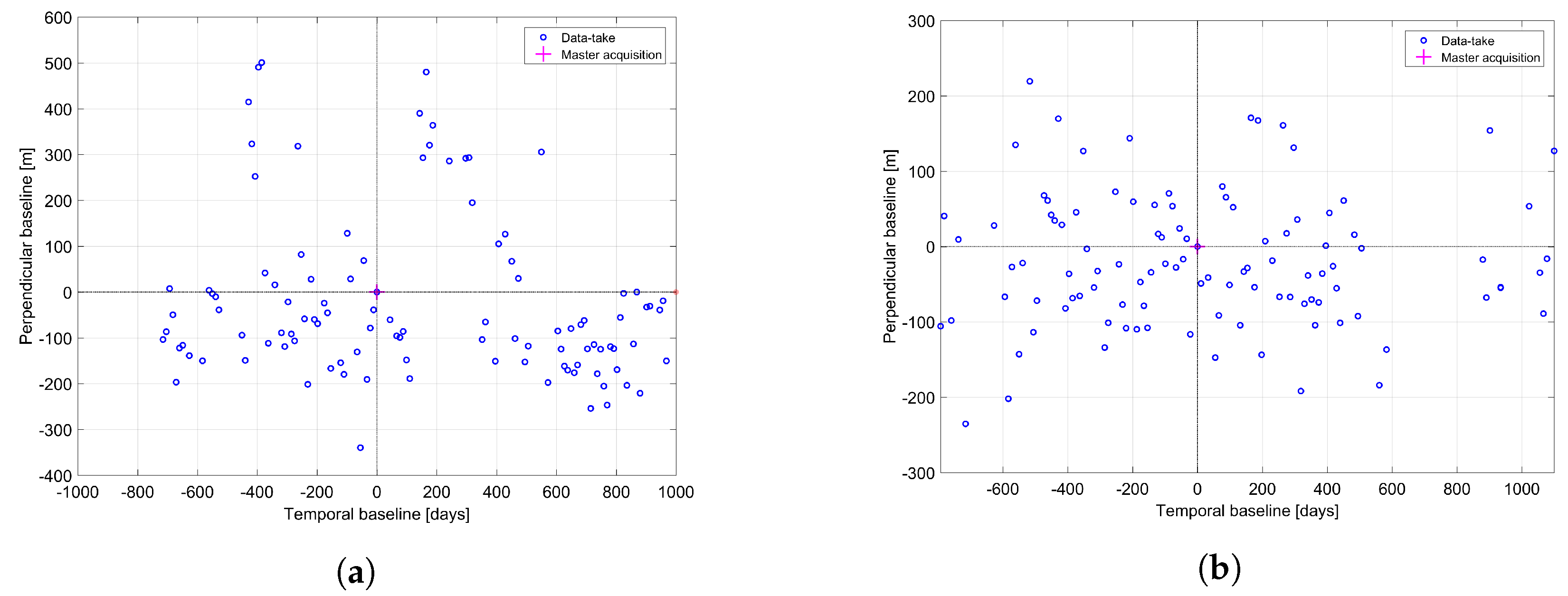
5.1. Berlin InSAR and PSI Processing

The two stacks of Berlin have undergone InSAR and PSI processing using the PSI-GENESIS of the German Aerospace Center (DLR) [38,39,40,41]. The master scenes for both stacks are chosen in winter, on 24 December 2011 for beam 57 and on 7 March 2012 for beam 42, and central with respect to the temporal and perpendicular baselines. The baseline distribution of the SAR images of both beams can be seen in Figure 6. Prior to the InSAR stacking, complex SAR images are oversampled by a factor of two in both azimuth and range in order to avoid signal aliasing of the interferograms and amplitudes. The coregistration of slave images onto the master scene is carried out geometrically using a Shuttle Radar Topography Mission (SRTM) DEM and precise orbits and further applying an offset correction using PS [42]. Differential interferograms are then formed by removing the topographic phase contribution using the aforementioned DEM.

The PSI processing is initiated by extracting the PS candidates by thresholding on the SCR of the targets estimated in the coregistered SAR image stack [2,38]. After geocoding of the PS candidates using their corresponding DEM heights, a grid with cell size of 250 m is superimposed on all PS and the PS with the highest phase stability is selected within each cell using the locally estimated temporal coherence. These PS form the reference network, which is the basis for the estimation of height and deformation parameters as well as the estimation and removal of the atmospheric phase screen [1,2]. The parameters of interest in this study include DEM error, linear and periodic motion since we are analyzing an urban area with the acquisition time spanning over a few years. After the estimation of differential parameters on the arcs of the network, a robust ${\ell }_1$-norm network inversion for outlier rejection is carried out and a high quality PS is selected as the reference point [40]. Subsequently, the DEM error and the deformation at each point of the reference network are estimated using an ${\ell }_2$-norm network inversion relative to the previously selected reference point. After compensating the estimated APS, the PS that are not part of the reference network are connected to the nearest reference network points and their parameters are estimated. Later, the DEM height of each PS is added to its corresponding differential residual height estimate. The radar timing of each PS and its updated height are used for geocoding. The final results of the PSI processing are the topographic and deformation maps as well as displacement history of each PS. Since the focus of this paper is on geocoding accuracy of the point clouds only the topographic maps are reported. The results are shown in Figure 7 and Figure 8. The ascending and descending point clouds consist of approximately 1.3 and 1.4 million PS, respectively. The higher density of PS is seen along the railways and also on building façades. The white parts with no detected PS include mostly the vegetated areas such as the well known Tierpark situated at the lower left of the center of the scene. Deformation maps of Berlin obtained from TerraSAR-X PSI and SAR tomography have been previously analyzed [4,14,43,44] and are not further discussed here.

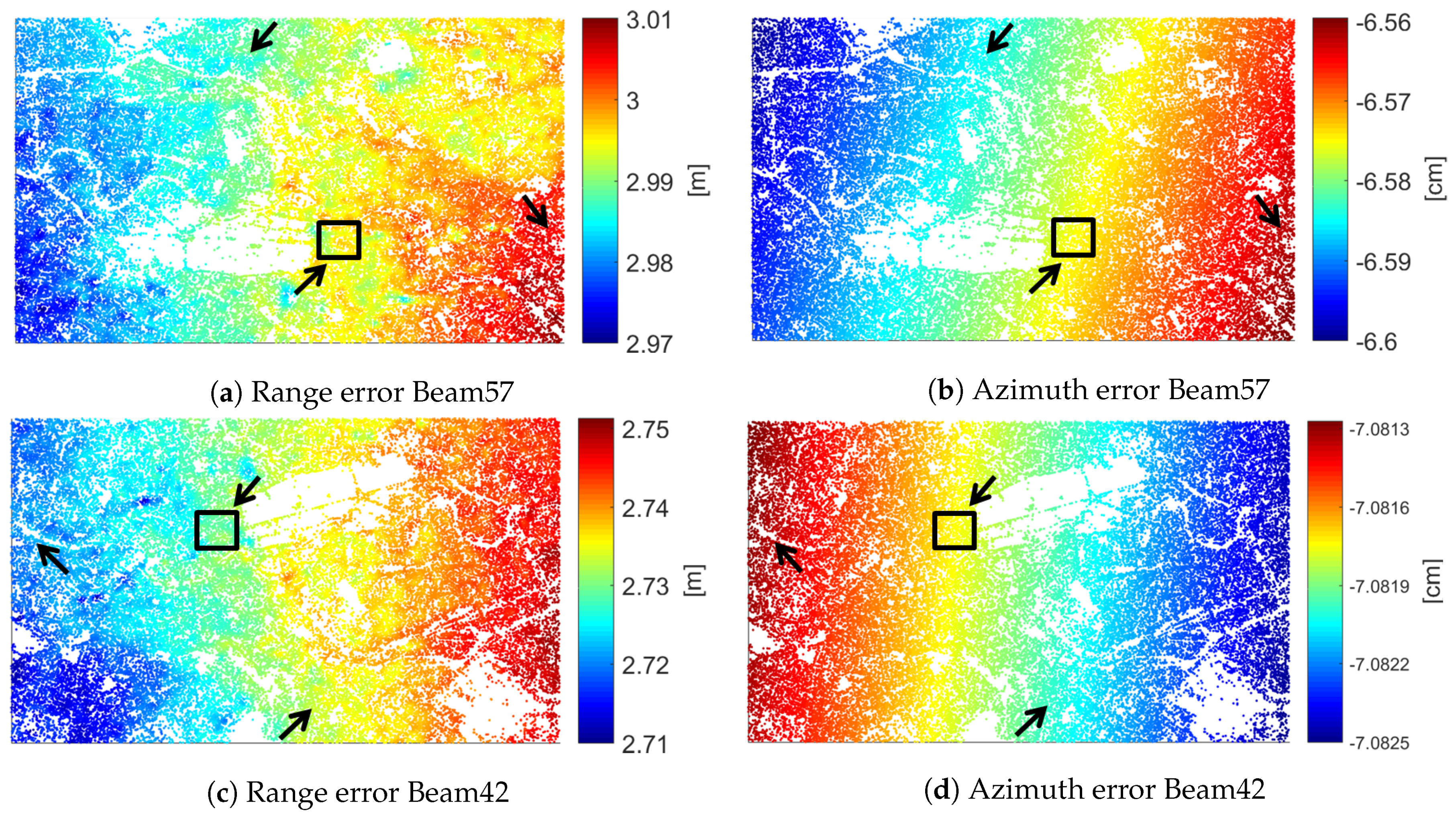
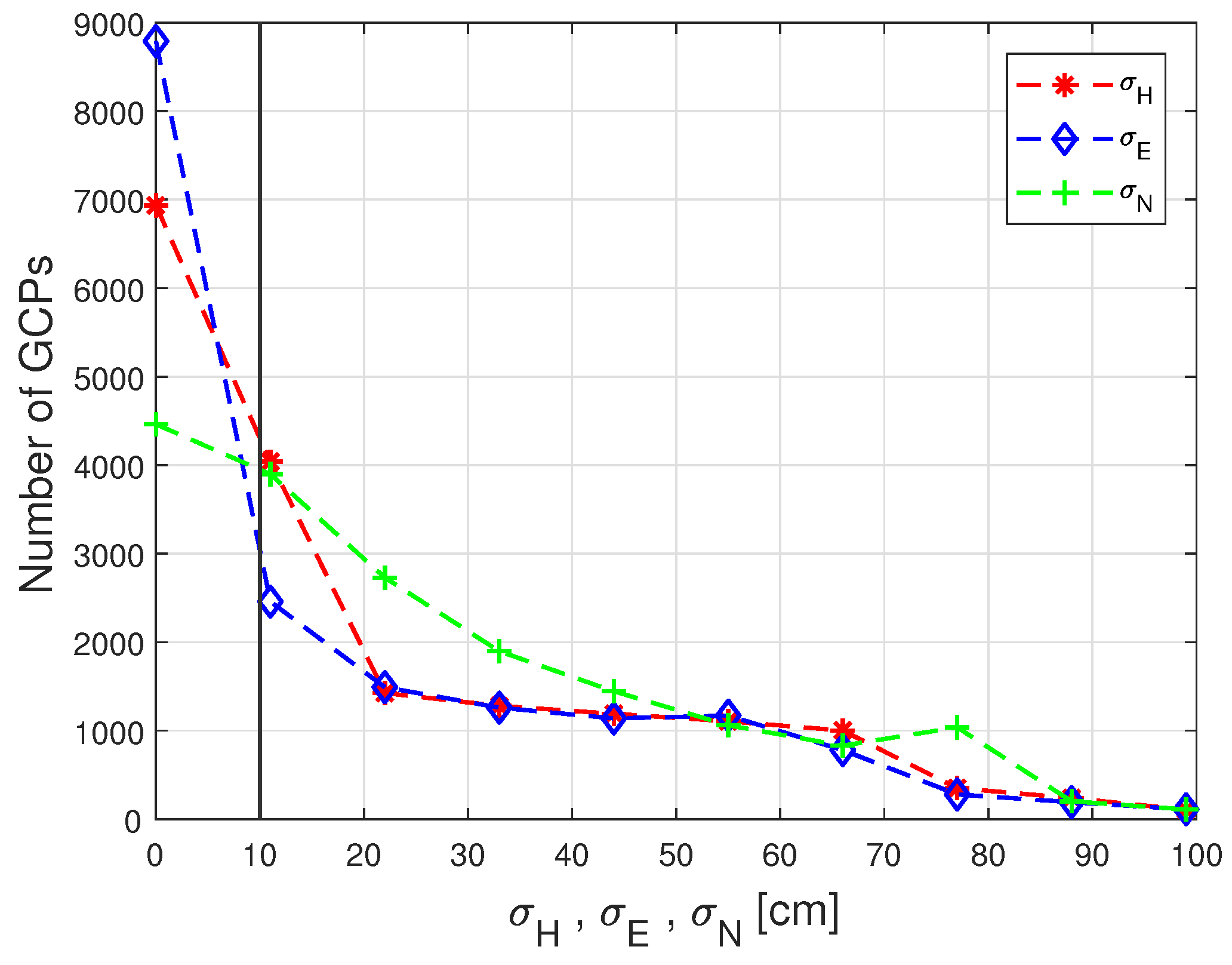
5.2. Geodetic Corrections, GCP Generation and Height Offset Estimation

Geodetic error corrections for individual SAR images and GCP generation have been carried out with the SAR Geodesy Processor (SGP) of the DLR [20,35]. All the timing corrections stated in Section 3.2 are evaluated for a coarse grid of 200 m in the slant range geometry. The sum of all corrections in the range and azimuth components of the master scene acquisitions of both beams are visualized in Figure 9. The corrections are in the radar coordinate system where, the y-axis represents the azimuth coordinate and the x-axis depicts the range coordinate. The errors are defined in the unit of length by multiplying range errors with $c/2$ for one-way measurements and azimuth errors with an average TerraSAR-X ground track velocity of 7050 m/s. It is seen that the magnitude of range errors is close to 3 m for Beam57 and approximately 2.75 m for Beam42, whereas the difference of maximum and minimum range errors over the scene is only 4 cm for both beams. The main contributions to the range errors come from the troposhperic error followed by geodynamic effects and finally the ionospheric delays. The azimuth errors are far less significant than range errors and manifest in sub-decimeter regimes, with millimeter variations across the scenes for both beams. The main source for azimuth errors is geodynamic effects followed by errors due to satellite dynamics. It is important to note that given the small squint angle of the TerraSAR-X high resolution spotlight products and their operation in X-band, the tropospheric and ionospheric delays are negligible for azimuth timings and therefore are not considered in the SAR imaging geodesy method [34].

For GCP generation, 27 images from both beams are selected, which have been acquired within a period of 12 months, in 2014 and at the beginning of 2015. The reason for the time restriction is avoiding the impact of plate tectonics on the final GCP coordinates. Bright point targets are precisely extracted from the SLCs using PTA with a maximum oversampling factor of 32 in both azimuth and range followed by a 2D kernel interpolation in a 3 × 3 window [27]. The signal path delays and geodetic errors are corrected for the location of each point target using their extracted timing information. After coarse geocoding of these points using a SRTM DEM, for each target, its corresponding points from other SLCs are detected if they are located within a distance of couple of meters relative to each other. The timing information of assumed identical targets are then combined through stereo SAR to estimate the absolute 3D coordinates of the GCP. The total number of GCPs localized from the combination of the aforementioned 27 SLCs is 17,673. The SGP removes all the GCPs with localization precision worse than 1 m based on the 1$\sigma$ rule. We further filter the results based on the posterior precision of GCP coordinates in the local East, North and ellipsoidal height. For precision values, we impose a threshold of 10 cm for all coordinate components. It is observed from Figure 10 that, by imposing the 10 cm threshold, there still remains an acceptable number of GCPs. This number is equal to 3800. As the final step, as was mentioned in Section 3.3, the GCPs are further filtered based on their closeness to the road network data of the scene, which reduces the number of GCPs to approximately 1000. The final obtained GCPs are visualized (in purple) on top of the geocoded PSI point clouds (in gray) in Figure 11. It is seen that the GCPs almost cover the full area within both PSI point clouds.

The generated SAR-GCPs are used to estimate the DEM error of the reference point of each PSI point cloud. For each radar-coded GCP, its closest PS with an ADI value lower than 0.4 is selected. The higher threshold value of 0.4 is preferred instead of the recommended ADI threshold of 0.25 [1], since lamp poles and traffic signs are assumed to be less stable than the more common PS which usually occur on building façades and corners. The correspondence detection is further refined by removing points which show large deviations with respect to the radar-coded GCPs (see Section 3.4). After the correspondence detection, the DEM error is estimated by analyzing the histogram of ellipsoidal height differences. Figure 12 summarizes the robust shift estimation procedure for both beams of Berlin. The left and right subfigures correspond to results from Beam57 and Beam42, respectively. The 2D scatterer plots show the distribution of range and azimuth coordinate differences among GCPs and their corresponding identified PS. In Figure 12a,b, the differences are plotted before outlier removal. It can be seen that very large deviations still occur after the correspondence detection step. Average deviations in the centimeter regime is observed in the range component while for the azimuth differences of Beam57, the mean deviation is close to 12 cm. The sample standard deviations, annotated in the subfigures, also show the large spread of the differences in both coordinate components in the meter regime. The second row of the subfigures, Figure 12c,d, depict the scatter plots after discarding outliers both in range and azimuth based on the $2\sigma$ rule. Note that the standard deviations for the outlier removal purpose are robustly estimated using MAD, as was explained in Section 3.4, while the annotated values in the subfigures are sample standard deviations, that are sensitive to outliers. From Figure 12c,d, it is clearly observed that the mean deviations decrease and now are close to 2 cm and 3 cm for range coordinate differences and approximately 2 cm and 1 cm for azimuth coordinate differences of Beam57 and Beam42, respectively. It is important to note that the radar coordinate differences have been compensated for the continental drift which occurred between the master acquisition times of each beam, in 2011 and 2012, and the epoch with respect to which the GCPs have been localized, in 2015. This coordinate shift has been computed utilizing the average East, North, Up velocities from the nearest International GNSS Service (IGS) permanent station, in Potsdam approximately 45 km away from Berlin, and have been projected into the line-of-sight and the azimuth directions of each beam. Eventually, the third row, Figure 12e,f shows the histogram of height differences among GCP-PS pairs after discarding observations based on the $2\sigma$ rule. The peaks of the smoothed version of the height difference histograms provide the robust estimates of the DEM errors which are −4.06 m and −6.27 m for Beam57 and Beam42, respectively. It is expected that the DEM errors have different values because of non-identical PSI reference points. The estimated height shifts are subtracted from the final height estimates of PSI and along with the fully corrected range and azimuth timings, using SGP, an updated geocoding is carried out for each beam separately. The localization accuracy of the corrected point clouds are evaluated in the next subsection.

5.3. Cross-Comparison with LiDAR

The geocoded PSI point clouds before and after applying the aforementioned corrections are compared with the reference LiDAR data. It is important to note that, since an objective comparison is difficult to perform, due to the inherent differences between LiDAR and PSI point clouds, we avoid using the term validation and therefore reside with the word cross-comparison.

In 2D, the corrected and non-corrected PSI point clouds of ascending and descending tracks are overlaid on the LiDAR data. For a few individual buildings, their façade PS are extracted by the method explained in Section 3.5. For this procedure, the neighborhood size is chosen to be 4 m while the height variance threshold is 1.5 m as recommended by [14]. The results for three buildings, indicated with cyan arrows in Figure 5, are visualized in Figure 13. The green and red dots display the PS from ascending and descending point clouds, respectively, while the white dots show the extracted building footprints from LiDAR. All data points are presented in the UTM projection. The first and second rows correspond to the non-corrected and corrected results, respectively. Note that the subfigures have different scales. It is clearly seen that, before applying the geodetic corrections and DEM error compensation, red dots are located far away from the building footprints. This 2D shift is largely compensated after applying the corrections in all the three cases. Moreover, the endpoint of each façade in the corrected point clouds match with the endpoint of the façade from the point cloud from the opposing geometry. This is not the case for non-corrected point clouds. Another observation is related to the ascending point clouds. The 2D shift imposed on the green point cloud after correction is much smaller than the red point cloud. One of the reasons is that the DEM error of the ascending point cloud is approximately two meters smaller than the descending point cloud. Another explanation for this is that the center incidence angle is smaller for the descending point cloud compared to the ascending one (see Table 1). Therefore, according to Equations (8) and (11), the horizontal shifts are larger for the descending point cloud as has been expected.

In order to quantify the approximate deviation of each point cloud from the reference LiDAR data, the distance of each façade PS was calculated with respect to a 2D line fitted to the corresponding LiDAR façade of all the three cases reported in Figure 13. The mean value of the distances for the corrected point clouds and the non-corrected point clouds are 0.4 m and 2.44 m, respectively. This proves that applying the corrections have certainly improved the overall geocoding accuracy of the PSI point clouds in the horizontal plane as the corrected point clouds are located closer to the LiDAR footprints compared to the non-corrected ones. It is important to note that a deviation equal to zero does not necessarily mean that the PSI point cloud is absolutely without any errors. The reason is that façade PS originate as triple-bounces from window corners of buildings which are not perfectly aligned with footprints extracted from LiDAR. Therefore, the difference in viewing geometries of both sensors does not allow a flawless comparison.

For the 1D vertical accuracy analysis, we first visually inspect the vertical cross-section of corrected and non-corrected PSI point clouds overlaid onto their corresponding LiDAR point cloud for a test site. Figure 14 visualizes this cross-section. In the subfigures, the x- and y-axes correspond to the UTM Easting and ellipsoidal heights, respectively. The red and green colors represent the PSI point clouds of Beam42 and Beam57 while the reference LiDAR point clouds are in white. In the LiDAR data, the ground line and the building roofs are easily distinguishable as they contain the majority of the points and are seen as very bright lines in the figures. By looking at Figure 14a,c, a clear height offset between the ground lines in the non-corrected PSI point clouds of both beams and the ground line in the LiDAR data is observed. Moreover, in the non-corrected point clouds, the PS on buildings are not seamlessly aligned with building roofs of the LiDAR point clouds. The non-identical height shifts are compensated by employing the height offset estimation method, relying on SAR GCPs, as it can be seen in Figure 14b,d.

In order to quantify the degree of improvement in the absolute height of PSI point clouds with respect to the LiDAR heights, the façade PS are excluded and height histograms are formed following the approach described in Section 3.5. This procedure is carried out for a subset of the PSI point clouds and their corresponding LiDAR data marked with yellow rectangle in Figure 5. The ellipsoidal height histograms are reported in Figure 15 where the top and bottom subfigures correspond to Beam57 and Beam42, respectively.

The red, green and blue colors describe the height histograms of the LiDAR, non-corrected PSI and corrected PSI point clouds. The first peak of the histograms relates to the ground points. It is observed that, after the DEM error of the reference point is estimated with the use of SAR-GCPs, the height histograms of the corrected PSI point clouds move toward the height histograms of the LiDAR data. Within each histogram, the height of the ground peaks are reported. The absolute differences in the height at the peaks of the non-corrected point clouds with respect to the peak of the LiDAR data are approximately 3.96 m and 6.43 m for Beam57 and Beam42, respectively. The differences reduce to 0.21 m and 0.11 m after the proposed height offset compensation method has been applied.

6. Conclusions

In this paper, a SAR-based method has been introduced in order to improve the geocoding accuracy of PSI point clouds. It has been shown that the geocoding errors related to height can be compensated for by the use of GCPs which are extracted and localized using the SAR data itself. The corrections in range and azimuth timings of the PS also influence the horizontal accuracy and have been fully considered using the SAR imaging geodesy technique. The method does not rely on any external positioning data and can be carried out as a post-processing step after PSI point cloud generation. A few test cases have been visually inspected, which showed the significance of the applied corrections, especially for the estimation of the DEM error of PSI reference points. By cross-comparison of corrected PSI point clouds with respect to a reference LiDAR data, it has been shown that a 2D horizontal accuracy around 40 cm is achievable while the height accuracy was reported to be close to 20 cm for one beam and 10 cm for the other beam. The improvement in the geocoding accuracy is highly beneficial for very localized small-scale deformation monitoring when, for instance, a certain part of an individual building is of interest rather than a large area surrounding it. PSI products with high localization accuracy can also be more easily compared with or incorporated into data from other sensors in comparison with the out-of-the-box PSI results.

Although the described methodology has been applied to high resolution X-band SAR data, the concept of geodetic corrections using SAR imaging geodesy is applicable to medium resolution products, such as the ones from the Sentinel-1 C-band SAR images, as well. The main limitation of the proposed method for lower resolution SAR products is related to the GCP identification part. In this case, the SCR of good GCP candidates should be high enough so that they can be visible in medium and low resolution SAR images. We are currently investigating this issue on Sentinel-1 images of urban areas. It is also noteworthy that the explained method is mostly suitable for urban areas where a large number of PS and GCPs are expected. However, in rural areas close to road networks, where lamp poles and traffic lights are also available, the exact same workflow explained in this paper can be used for geocoding error correction.

Future studies will focus on the integration of SAR-GCPs inside the PSI processing chain. Furthermore, more sophisticated and objective comparison strategies should be introduced for validation of PSI results with respect to accurate DSMs.

References

1. Ferretti, A.; Prati, C.; Rocca, F. Permanent scatterers in SAR interferometry. IEEE Trans. Geosci. Remote Sens. 2001, 39, 8–20. [Google Scholar] [CrossRef] [Green Version]
2. Kampes, B.M. Radar Interferometry: Persistent Scatterer Technique. In Number v. 12 in Remote Sensing and Digital Image Processing; Springer: Dordrecht, The Netherlands, 2006. [Google Scholar]
3. Zebker, H.; Villasenor, J. Decorrelation in interferometric radar echoes. IEEE Trans. Geosci. Remote Sens. 1992, 30, 950–959. [Google Scholar] [CrossRef] [Green Version]
4. Gernhardt, S.; Bamler, R. Deformation monitoring of single buildings using meter-resolution SAR data in PSI. ISPRS J. Photogramm. Remote Sens. 2012, 73, 68–79. [Google Scholar] [CrossRef]
5. Gernhardt, S.; Adam, N.; Eineder, M.; Bamler, R. Potential of very high resolution SAR for persistent scatterer interferometry in urban areas. Ann. GIS 2010, 16, 103–111. [Google Scholar] [CrossRef]
6. Schwabisch, M. A fast and efficient technique for SAR interferogram geocoding. In Proceedings of the 1998 IEEE International Geoscience and Remote Sensing (IGARSS), Seattle, WA, USA, USA, 6–10 July 1998; Volume 2, pp. 1100–1102. [Google Scholar] [CrossRef]
7. Hanssen, R.F. Radar Interferometry: Data Interpretation and Error Analysis. In Number v. 2 in Remote Sensing and Digital Image Processing; Kluwer Academic: Dordrecht, The Netherlands; Boston, MA, USA, 2001. [Google Scholar]
8. Eineder, M. Efficient simulation of SAR interferograms of large areas and of rugged terrain. IEEE Trans. Geosci. Remote Sens. 2003, 41, 1415–1427. [Google Scholar] [CrossRef]
9. Eineder, M.; Minet, C.; Steigenberger, P.; Cong, X.Y.; Fritz, T. Imaging Geodesy—Toward Centimeter-Level Ranging Accuracy With TerraSAR-X. IEEE Trans. Geosci. Remote Sens. 2011, 49, 661–671. [Google Scholar] [CrossRef]
10. Chang, L.; Hanssen, R.F. Detection of cavity migration and sinkhole risk using radar interferometric time series. Remote Sens. Environ. 2014, 147, 56–64. [Google Scholar] [CrossRef]
11. Yang, M.; Dheenathayalan, P.; Chang, L.; Wang, J.; Lindenbergh, R.; Liao, M.; Hanssen, R. High-precision 3D geolocation of persistent scatterers with one single-Epoch GCP and LIDAR DSM data. In Proceedings of the Living Planet Symposium; European Space Agency: Paris, France, 2016; Volume 740, p. 398. [Google Scholar]
12. Bateson, L.; Novali, F.; Cooksley, G. Terrafirma User Guide: A Guide to the Use and Understanding of Persistent Scatterer Interferometry in the Detection and Monitoring of Terrain-Motion; Technical Report 19366/05/I-EC; ESA: Paris, France, 2010. [Google Scholar]
13. Gernhardt, S.; Cong, X.Y.; Eineder, M.; Hinz, S.; Bamler, R. Geometrical Fusion of Multitrack PS Point Clouds. IEEE Geosci. Remote Sens. Lett. 2012, 9, 38–42. [Google Scholar] [CrossRef]
14. Gernhardt, S. High Precision 3D Localization and Motion Analysis of Persistent Scatterers Using Meter-Resolution Radar Satellite Data. Ph.D. Thesis, Technische Universität München, München, Germany, 2012. [Google Scholar]
15. Cong, X. SAR Interferometry for Volcano Monitoring: 3D-PSI Analysis and Mitigation of Atmospheric Refractivity. Ph.D. Thesis, Technische Universität München, München, Germany, 2014. [Google Scholar]
16. Besl, P.; McKay, N.D. A method for registration of 3-D shapes. IEEE Trans. Pattern Anal. Mach. Intell. 1992, 14, 239–256. [Google Scholar] [CrossRef]
17. Zhu, X.X.; Montazeri, S.; Gisinger, C.; Hanssen, R.F.; Bamler, R. Geodetic SAR Tomography. IEEE Trans. Geosci. Remote Sens. 2016, 54, 18–35. [Google Scholar] [CrossRef]
18. Gisinger, C.; Balss, U.; Pail, R.; Zhu, X.X.; Montazeri, S.; Gernhardt, S.; Eineder, M. Precise Three-Dimensional Stereo Localization of Corner Reflectors and Persistent Scatterers With TerraSAR-X. IEEE Trans. Geosci. Remote Sens. 2015, 53, 1782–1802. [Google Scholar] [CrossRef]
19. Zhu, X.X.; Bamler, R. Very high resolution spaceborne SAR tomography in urban environment. IEEE Trans. Geosci. Remote Sens. 2010, 48, 4296–4308. [Google Scholar] [CrossRef] [Green Version]
20. Balss, U.; Runge, H.; Suchandt, S.; Cong, X.Y. Automated extraction of 3-D Ground Control Points from SAR images—An upcoming novel data product. In Proceedings of the 2016 IEEE International Geoscience and Remote Sensing Symposium (IGARSS), Beijing, China, 10–15 July 2016; pp. 5023–5026. [Google Scholar] [CrossRef]
21. Montazeri, S.; Gisinger, C.; Eineder, M.; Zhu, X.X. Automatic Detection and Positioning of Ground Control Points Using TerraSAR-X Multiaspect Acquisitions. IEEE Trans. Geosci. Remote Sens. 2018, 56, 2613–2632. [Google Scholar] [CrossRef]
22. Van Leijen, F. Persistent Scatterer Interferometry Based on Geodetic Estimation Theory. Ph.D. Thesis, Delft University of Technology, Delft, The Netherlands, 2014. [Google Scholar]
23. Cumming, I.G.; Wong, F.H.C. Digital Processing of Synthetic Aperture Radar Data: Algorithms and Implementation; Artech House Remote Sensing Library, Artech House: Boston, MA, USA, 2005. [Google Scholar]
24. Yoon, Y.; Eineder, M.; Yague-Martinez, N.; Montenbruck, O. TerraSAR-X Precise Trajectory Estimation and Quality Assessment. IEEE Trans. Geosci. Remote Sens. 2009, 47, 1859–1868. [Google Scholar] [CrossRef]
25. Hackel, S.; Montenbruck, O.; Steigenberger, P.; Balss, U.; Gisinger, C.; Eineder, M. Model improvements and validation of TerraSAR-X precise orbit determination. J. Geod. 2017, 91, 547–562. [Google Scholar] [CrossRef]
26. Cong, X.Y.; Balss, U.; Eineder, M.; Fritz, T. Imaging Geodesy—Centimeter-Level Ranging Accuracy with TerraSAR-X: An Update. IEEE Geosci. Remote Sens. Lett. 2012, 9, 948–952. [Google Scholar] [CrossRef]
27. Balss, U.; Cong, X.Y.; Brcic, R.; Rexer, M.; Minet, C.; Breit, H.; Eineder, M.; Fritz, T. High precision measurement on the absolute localization accuracy of TerraSAR-X. In Proceedings of the 2012 IEEE International Geoscience and Remote Sensing Symposium, Munich, Germany, 22–27 July 2012; pp. 1625–1628. [Google Scholar] [CrossRef]
28. Balss, U.; Gisinger, C.; Cong, X.Y.; Brcic, R.; Hackel, S.; Eineder, M. Precise measurements on the absolute localization accuracy of TerraSAR-X on the base of far-distributed test sites. In Proceeding of the 10th European Conference on Synthetic Aperture Radar (EUSAR), Berlin, Germany, 3–5 June 2014. [Google Scholar]
29. Balss, U.; Breit, H.; Fritz, T.; Steinbrecher, U.; Gisinger, C.; Eineder, M. Analysis of internal timings and clock rates of TerraSAR-X. In Proceedings of the 2014 IEEE International Geoscience and Remote Sensing Symposium, Quebec City, QC, Canada, 13–18 July 2014; pp. 2671–2674. [Google Scholar] [CrossRef]
30. Misra, P.; Enge, P. Global Positioning System: Signals, Measurements, and Performance; Misra, P., Enge, P., Eds.; Jamuna Press: Warsaw, Poland, 2006. [Google Scholar]
31. Gisinger, C. Atmospheric Corrections for TerraSAR-X Derived from GNSS Observations. Master’s Thesis, Technische Universität München, München, Germany, 2012. [Google Scholar]
32. Balss, U.; Gisinger, C.; Cong, X.Y.; Brcic, R.; Steigenberger, P.; Eineder, M.; Pail, R.; Hugentobler, U. High resolution geodetic earth observation with TerraSAR-X: Correction schemes and validation. In Proceedings of the 2013 IEEE International Geoscience and Remote Sensing Symposium, Melbourne, VIC, Australia, 21–26 July 2013; pp. 4499–4502. [Google Scholar] [CrossRef]
33. Petit, G.; Luzum, B. IERS Conventions; IERS Technical Note No. 36; Verlag des Bundesamts für Kartographie und Geodäsie: Frankfurt am Main, Germany, 2010. [Google Scholar]
34. Balss, U.; Gisinger, C.; Eineder, M. Measurements on the Absolute 2-D and 3-D Localization Accuracy of TerraSAR-X. Remote Sens. 2018, 10, 656. [Google Scholar] [CrossRef]
35. Eineder, M.; Balss, U.; Suchandt, S.; Gisinger, C.; Cong, X.; Runge, H. A definition of next-generation SAR products for geodetic applications. In Proceedings of the 2015 IEEE International Geoscience and Remote Sensing Symposium, Milan, Italy, 26–31 July 2015; pp. 1638–1641. [Google Scholar] [CrossRef]
36. OpenStreetMap Contributors. Planet Dump. 2017. Available online: https://www.openstreetmap.org (accessed on 18 August 2018).
37. Rousseeuw, P.J.; Hubert, M. Anomaly detection by robust statistics. Wiley Interdiscip. Rev. Data Min. Knowl. Discov. 2018, 8, 1–14. [Google Scholar] [CrossRef]
38. Adam, N.; Kampes, B.M.; Eineder, M. The development of a scientific persistent scatterer system: Modifications for mixed ERS/ENVISAT time series. In Proceedings of the Envisat and ERS Symposium, Salzburg, Austria, 6–10 September 2004; pp. 1–9. [Google Scholar]
39. Adam, N.; Gonzalez, F.R.; Parizzi, A.; Brcic, R. Wide area Persistent Scatterer Interferometry: Current developments, algorithms and examples. In Proceedings of the 2013 IEEE International Geoscience and Remote Sensing Symposium, Melbourne, VIC, Australia, 21–26 July 2013; pp. 1857–1860. [Google Scholar] [CrossRef]
40. Rodriguez Gonzalez, F.; Bhutani, A.; Adam, N. L1 network inversion for robust outlier rejection in persistent Scatterer Interferometry. In Proceedings of the 2011 IEEE International Geoscience and Remote Sensing Symposium, Vancouver, BC, Canada, 24–29 July 2011; pp. 75–78. [Google Scholar] [CrossRef]
41. Rodriguez Gonzalez, F.; Adam, N.; Parizzi, A.; Brcic, R. The Integrated Wide Area Processor (IWAP): A Processor for Wide Area Persistent Scatterer Interferometry. In Proceedings of the ESA Living Planet Symposium 2013; ESA: Edinburgh, UK, 2013; pp. 1–4. [Google Scholar]
42. Adam, N.; Kampes, B.M.; Eineder, M.; Worawattanamateekul, J.; Kircher, M. The Development of a Scientific Permanent Scatterer System. In Proceedings of the Joint ISPRS/EARSeL Workshop on High Resolution Mapping from Space 2003, Edinburgh, UK, 9–13 September 2003. [Google Scholar]
43. Montazeri, S. The Fusion of SAR Tomography and Stereo-SAR for 3D Absolute Scatterer Positioning. Master’s Thesis, Delft University of Technology, Delft, The Netherlands, 2014. [Google Scholar]
44. Montazeri, S.; Zhu, X.X.; Eineder, M.; Bamler, R. Three-Dimensional Deformation Monitoring of Urban Infrastructure by Tomographic SAR Using Multitrack TerraSAR-X Data Stacks. IEEE Trans. Geosci. Remote Sens. 2016, 54, 6868–6878. [Google Scholar] [CrossRef]
Figure 1. Timing bias in azimuth and its effect on the geocoded coordinates. (a) azimuth timing error causing a displacement on the ground δ l a z ; (b) projection of δ l a z onto the East δ l a z E and North δ l a z N components using satellite heading angle α .
Remotesensing 10 01523 g001
Figure 2. Timing bias in range and its effect on the geocoded coordinates. (a) range timing error and its impact on geocoding in the ground range δ l g r ; (b) projection of δ l g r onto the East δ l g r E and North δ l g r N components using satellite heading angle α .
Remotesensing 10 01523 g002
Figure 3. Depiction of height error δ H due to unknown DEM error at the reference point and its effect on geocoded coordinates. It can be seen that this error causes a shift in the cross-range direction δ l H s , which is decomposed into an offset in ground range δ l H g r and a vertical component δ H .
Remotesensing 10 01523 g003
Figure 4. Workflow of the utilized geocoding error correction method. The processing steps, included in the big rectangles, are carried out independently and their results are shown by the parallelograms. The double shapes indicate that each processing is carried out for two or more SAR image stacks, which is the necessary condition for GCP generation.
Remotesensing 10 01523 g004
Figure 5. Optical image of Berlin taken from Google Earth. The mean scene coverage of the TerraSAR-X images as well as the extent of the LiDAR data are marked with colored rectangles. The small yellow rectangle shows the test site within which the vertical localization accuracy of PSI point clouds has been analyzed. The cyan arrows indicate the three test sites used for horizontal accuracy analysis.
Remotesensing 10 01523 g005
Figure 6. Temporal-perpendicular baseline distribution of the SAR image stacks in Berlin. (a,b) correspond to the data stacks of Beam57 and Beam42, respectively.
Remotesensing 10 01523 g006
Figure 7. Geocoded PSI point cloud of Berlin, reconstructed from Beam57, in UTM coordinates. The ellipsoidal height is colorcoded. The x- and y-axis correspond to the UTM East and North, respectively. The test sites used for vertical and horizontal accuracy analysis are marked with black rectangle and black arrows, respectively.
Remotesensing 10 01523 g007
Figure 8. Geocoded PSI point cloud of Berlin, reconstructed from Beam42, in UTM coordinates. The ellipsoidal height is colorcoded. The x- and y-axis correspond to the UTM East and North, respectively. The test sites used for vertical and horizontal accuracy analysis are marked with black rectangle and black arrows, respectively.
Remotesensing 10 01523 g008
Figure 9. Range and azimuth error in the radar coordinate system (x-axis: range, y-axis: azimuth) of the master scenes of both investigated beams, which were acquired on 24 December 2011 (Beam57) and on 7 March 2012 (Beam42). Note that the scale of the colorbars for range error is in meters while the one for azimuth errors is in centimeters. The test sites used for vertical and horizontal accuracy analysis are marked with black rectangle and black arrows, respectively.
Remotesensing 10 01523 g009
Figure 10. Histogram of GCP precision values in East σ E , North σ N and height σ H .
Remotesensing 10 01523 g010
Figure 11. Distribution of the GCPs within the PSI point clouds of both beams. The test sites used for vertical and horizontal accuracy analysis are marked with black rectangle and black arrows, respectively.
Remotesensing 10 01523 g011
Figure 12. Restriction of the DEM error estimation to the true correspondences among GCPs and PS. (a,b) demonstrate the scatterplots of GCP-PS pairs before outlier removal, for Beam57 and Beam42, respectively; (c,d) show the scatterplots of the GCP-PS pairs after outlier removal. This causes a decrease in the bias and the standard deviation of the coordinate differences; (e,f) depict the robust height offset estimation after removal of the height differences in accordance with the 2 σ rule. The peak of the smoothed histogram indicates the DEM error for each beam. Note that, for all the figures, the coordinate differences are defined as the GCP coordinates subtracted from their corresponding PS coordinates.
Remotesensing 10 01523 g012
Figure 13. 2D horizontal localization accuracy analysis of PSI point clouds of the test sites marked with cyan arrows in Figure 5 (top: non-corrected, bottom: corrected). The x- and y-axes correspond to the Easting and Northing in UTM. Green and red dots show the ascending and descending point clouds while white dots show the extracted LiDAR footprints. The scale of figures is not identical meaning that the degree of zoom-in is higher in subfigures (c,f).
Remotesensing 10 01523 g013
Figure 14. 1D vertical localization accuracy analysis of PSI point clouds, before and after applying geodetic corrections and height offset compensation, in comparison with LiDAR. The x- and y-axes correspond to the Easting in UTM and ellipsoidal height, respectively. Green and red dots show the ascending (Beam57) and descending (Beam42) point clouds while white dots show the LiDAR data. (a,c) depict the non-corrected point clouds while (b,d) correspond to the corrected ones. The height shifts, caused by the unknown DEM error of the reference points are easily recognizable in non-corrected point clouds while the offsets are compensated for in the corrected results. Note that the Easting and the height are differently scaled in order to emphasize the vertical effect.
Remotesensing 10 01523 g014
Figure 15. Ellipsoidal height histograms of non-façade points in LiDAR (red), non-corrected PSI (green) and corrected PSI point clouds (blue) corresponding to the yellow bounding box in Figure 5. (a,b) show the results for Beam57 and Beam42, respectively. For both beams, the height shifts are compensated for after correction, using SAR-GCPs, as the ground peaks of PSI point clouds and LiDAR data become aligned.
Remotesensing 10 01523 g015