3D Convolutional Neural Networks for Crop Classification with Multi-Temporal Remote Sensing Images

Abstract

This study describes a novel three-dimensional (3D) convolutional neural networks (CNN) based method that automatically classifies crops from spatio-temporal remote sensing images. First, 3D kernel is designed according to the structure of multi-spectral multi-temporal remote sensing data. Secondly, the 3D CNN framework with fine-tuned parameters is designed for training 3D crop samples and learning spatio-temporal discriminative representations, with the full crop growth cycles being preserved. In addition, we introduce an active learning strategy to the CNN model to improve labelling accuracy up to a required threshold with the most efficiency. Finally, experiments are carried out to test the advantage of the 3D CNN, in comparison to the two-dimensional (2D) CNN and other conventional methods. Our experiments show that the 3D CNN is especially suitable in characterizing the dynamics of crop growth and outperformed the other mainstream methods.

1. Introduction

Benefiting from the huge number of high-quality spectral-temporal images captured from Earth observation satellites, or unmanned aerial vehicles (UAV), automatic crop classification [1,2] is becoming a fundamental technology for yield estimation, economic assessment, crop transportation, etc. Conventional classification methods, such as support vector machine (SVM) [3], K-nearest neighbor (KNN) [4], maximum likelihood classification (MLC) [5], etc., have been successfully applied in crop classification. However, these methods may be insufficient under the circumstances vegetation, etc. For example, many agricultural sectors of Chinese local governments are doing heavy manual labelling work to assure accurate reports. Therefore, it is still very important to develop new crop classification technologies.

Classification methods in remote sensing mainly consider two aspects, a feature extractor that transforms spatial, spectral, and/or temporal data into discriminative feature vectors, and a classifier that labels each feature vector to certain types. For crop or vegetation classification, the spatial and spectral features are typically extracted in two ways. One is to aggregate spectral bands into vegetation indices that represent the physical characteristics of vegetation, within which the normalized difference vegetation index (NDVI) is mostly used. Wardlow et al. analyzed the time-series MODIS 250 m enhanced vegetation index (EVI) and NDVI datasets for crop classification [1]. Xiao et al. utilized NDVI, EVI and land surface water index (LSWI) aggregated from MODIS temporal images to discriminate rice from cloud, water, and evergreen plants [6]. Conrad et al. divided MODIS 250 m NDVI time series into several temporal segments, from which metrics were derived as input features for crop classification [7]. Sexton et al. utilized humidity, luminance, NDVI, and their changes extracted from multi-temporal Landsat TM-5 images to classify land cover [8]. Simonneaux et al. produced NDVI profiles from a time series of ten radiometrically corrected Landsat TM images, and used the profiles to identify four crop types [9]. In [10], tasselled cap indices extracted from bi-temporal ASTER data were utilized for classifying crop rotations of cotton, winter wheat, and rice. In [11], a subset of features was selected out by random forest from 71 multiseasonal spectral and geostatistical features computed from RapidEye time series, to achieve the best crop classification accuracy. The other is to directly use original multi-temporal images for classification. Zhu and Liu classified the plant types of a forest using five Landsat TM-5 images and two Landsat TM-7 images of different times [12]. Guerschman et al. analyzed the performances of original images and NDVI on a land cover classification from multi-temporal Landsat images, and showed that better accuracy could be obtained by using all the temporal and spectral bands than using NDVI [13]. Esch et al. used both the multi-seasonal IRS-P6 satellite imagery and the derived NDVI based seasonality indices for crop type classification and a cropland and grassland differentiation [14].

In addition to spatio-temporal images, other remote sensing data, such as polarimetric synthetic aperture radar (SAR) images, with texture features extracted from them [15], are also utilized as inputs for a crop classification. McNairn et al. tested PALSAR multipolarization and polarimetric data for crop classification and found their performance to be competitive with that of temporal Landsat images [16].

As to classifier, SVM [3,11], KNN [4], MLC [5], artificial neural network (ANN) [5,17], decision tree [9,14], and random forest [18] are commonly used for vegetation classification. Murthy et al. compared a MLC, iterative-MLC, Principal Component Analysis (PCA) based MLC, and ANN for wheat extraction from multi-temporal images, and pointed out that ANN performed the better results [5]. Zhu and Liu utilized a hierarchical classification strategy and a recursive SVM framework to obtain a tree-type forest map [12]. Omkar et al. utilized a combination of multiple classification technologies, including MLC, particle swarm optimization (PSO), and ant colony optimization (ACO) for crop classification from a high-resolution satellite image [19]. Gallego et al. assessed the efficiency of different classification algorithms, including neural networks, decision trees, and support vector machines for crop classification based on a time series of satellite images [20]. Siachalou et al. used Hidden Markov Models (HMM) to set a dynamic model per crop type to represent the biophysical processes of an agricultural land [21].

In recent years, deep learning has been widely used and has become mainstream in artificial intelligence and machine learning [22]. Deep learning is a representation-learning method that can automatically learn internal feature representations with multiple levels from original images instead of empirical feature design, and has proved to be very efficient in image classification and object detection. In contrast, vegetation indices such as NDVI only use several bands and may lead to low performance in complicated situations, e.g., crop classification where the spectrums, periods, geometry, and the interactions of various types of crops might be considered. Whereas, original temporal images used as feature input could contain noises or unfavorable information that decrease the performance of a classifier.

The main objective of our study is to represent distinctive spatio-temporal features of crops by deep learning. In recent years, studies that were related to convolutional neural network (CNN) has been successfully applied in handwriting recognition from binary images [23], labelling from mainstream RGB image set [24], classification from multi-spectral or hyperspectral data [25], learning from videos [26], classification of brain magnetic resonance imaging (MRI) data [27], etc. However, a traditional two-dimensional (2D) CNN, mainly designed for RGB images, lacks the ability to extract the third dimensional features accurately. A 2D convolution causes the extracted features in additional dimensions (i.e., spectral or temporal) of a layer to be averaged and collapsed to a scalar. To overcome this, Kussul et al. introduced two CNNs for crop classification, one 2D CNN for spatial feature learning, and the other one-dimensional (1D) CNN for spectral feature learning [28]. However, this strategy requires additional empirical processing to combine the learned features, and hurdles a full automatic representation learning procedure.

Three-dimensional (3D) convolution naturally suits to spatio-temporal presentations. Recently, some studies have utilized 3D CNN for learning spatio-temporal features from videos [29,30], learning 3D structures from LiDAR point clouds [31], or learning spatio-spectral presentations from hyperspectral images [32]. In general, 3D CNN is not as widely applied as 2D CNN, as the temporal dimension is usually not considered in computer vision and machine learning. Remote sensing images generally provide dynamic or temporal information, from which more information could be extracted. For example, the relations among multi-temporal pictures of a certain crop are explicit. The rice growth cycle includes germination, tillering, spike differentiation, heading and flowering, milking and a mature stage. But these temporal features are often partially ignored or represented by simplistic models. Some studies [5,12,13], simply concatenate temporal images to represent period information; while in [8], only images of early growing season, late growing season and dormant stage were selected. In theory, a proper 3D convolution can extract these spatial and temporal features simultaneously in a more delicate and rigorous manner other than a direct concatenation of reflectance images. In this study, we develop a 3D CNN framework to extract information for multi-temporal images and compare it to a 2D CNN and some conventional empirical methods as SVM, KNN, etc.

Deep learning requires sufficient manual samples that are difficult to be obtained in our situation when crop types, varieties of a certain type of crop, and planting season vary from time to time. To achieve a satisfactory learning result with limited samples and reduced amount of labor work, we introduce a semi-automatic semi-supervised active learning strategy [33]. Active learning is used to pick up the most helpful unlabeled samples (i.e., samples supposed to best improve model performance), according to their scores to each label predicted from the current CNN model, for manual checking, and model retraining, iteratively.

To our knowledge, 3D CNN has not been applied to crop classification using multi-spectral multi-temporal remote sensing images, and compared to 2D CNN and other conventional methods. In Section 2, we introduce a 3D convolutional kernel, 3D CNN structure, and an active learning strategy for crop classification. In Section 3, three tests are carried out to evaluate 3D CNN performance, as compared to 2D CNN and conventional methods. Discussions and conclusions are given in Section 4 and Section 5, respectively.

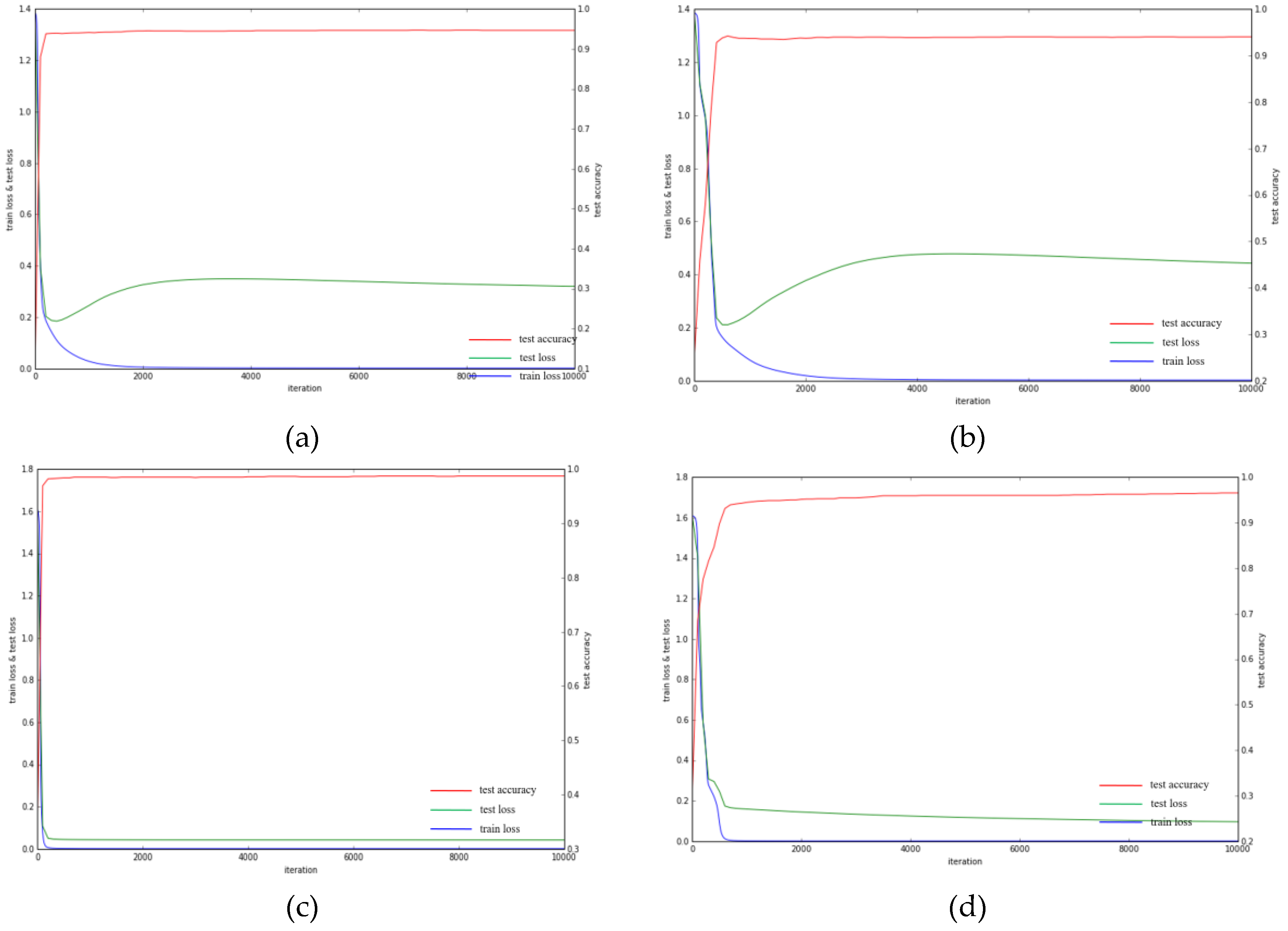
2. Methodology

2.1. 3D Convolution for Multi-Temporal Multi-Spectral Images

Deep CNN utilizes multi-layer linear transformation wx + b, followed by a non-linear activation σ, to learn multi-level representations of input data that are needed for the following classification or detection. In Equation (1), w is the weight template (i.e., convolution kernel), b is the bias vector of current layer l, and x is the neuron input from the previous layer l − 1. w and b are unknown parameters to be trained. The activation functions could be sigmoid or rectified linear unit (ReLU) [34].

y^l = σ(w^lx^l−1) + b^l

(1)

The form of original input x⁰ depends on special applications. In crop classification, x⁰ is typically collected from spectral-temporal images. A simple way is to treat all of the channels independently and clip same-size window patches around sample points or from shape files. A 2D convolution operation, as in Equation (2), is commonly used to aggregate raw information to a more abstract representation of next layer,

$$y_{cd}=\sigma ({\displaystyle \sum _{n=0}^N{\displaystyle \sum _{i=0}^M{\displaystyle \sum _{j=0}^M{w}_{ij,n}{x}_{(c+i)(d+j),n}}}}+b)$$

(2)

where w_ij,n is the n-th shared M × M weight template for a certain feature, N denotes the number of original channels or the feature maps of previous layer, x_cd and y_cd represent the input and output activation at location (c, d), respectively. For simplification, we omit the layer notation l in Equation (1).

To prevent a 2D convolution operation collapsing, all of the information from separate channels to a 2D plane (see Figure 1a), a 3D convolution as in Equation (3) can be used to extract and reserve the dynamic features through consecutive periods (see Figure 1b), and can be written as,

$$y_{cde}=\sigma ({\displaystyle \sum _n{\displaystyle \sum _{k=0}^N{\displaystyle \sum _{i=0}^M{\displaystyle \sum _{j=0}^M{w}_{kij,n}{x}_{c+i,d+j,e+k,n}}}}}+b)$$

(3)

where w_kij is a 3D tensor, k is the temporal indicator and N is its length, n indicates n-th feature map of previous layer, x_cde and y_cde are the input and output activation at location (c, d, e), respectively. In practice, temporal images also consist of multi-spectral channels, that is, spatial, spectral, and temporal dimensions form a four-dimensional (4D) tensor. To treat spatio-temporal information as main characteristic, the relations among spectral bands must be treated independent in 3D convolution, just as R, G and B bands in a conventional 2D CNN. As in Figure 2, all temporal images of a certain wave band, for example, red, are stacked up to form a 3D tensor, followed by a “green” stack. Indicator n in (3) equals the stack number in the first layer of a 3D CNN. Obviously, to treat spatio-spectral information as main feature, one should stack spectral images of a certain time first.

2.2. 3D CNN Structure for Spatio-Temporal Images

We take the widely used neural network structure developed by Oxford’s Visual Geometry Group (VGGnet) [35] as template to train a deep convolutional neural network where all 2D convolution operations are replaced by 3D convolution. Small-size kernel (especially, 3 × 3 in an image) is used to represent multi-level features, while the length of the temporal dimension can be set to 3, as in [30]. However, the kernel-size parameter is also fine-tuned in experiments. Layer number and kernel number of each layer typically depend on the capacity of inputs and complexity of problems. We chose a five-layer 3D convolutional network, with 32 or 64 kernels for all the experiments in this study, as is shown in Figure 3. The input consists of m independent channels (typically four, blue, green, red and near infrared), with size of n × w × h in temporal, width, and height directions, respectively. The first three layers consists of common convolution-pooling concatenation with 32, 32, 64 neurons to be learned sequentially. To best reserve the temporal information, i.e., the complete crop growth cycle, uncompressed till the first full connected layer (short as FC), 1 × 2 × 2 average pooling strategy is applied. The last FC layer, with dimension c × 1 where c the label number, is then fed to loss function, here, Maxout [36], to mark samples a score to each label. We set a fixed learning rate of 0.001 but set different random sampling strategies and batch size according to the sample capacity of different tests.

In addition to the 3D CNN, a conventional 2D CNN is also applied. The structure is shown in Figure 4, which is similar to the 3D CNN and facilitates the comparison between 2D and 3D CNN.

The network structures in Figure 3 and Figure 4 are used both for a classic training-test process by discrete samples and for pixelwise classification of the whole image. In both cases, the input patch is abstracted into multi-level representations to classify the central point of the patch. In Section 3.2 and Section 4 we will discuss the optimal patch size and mixed-pixel problem.

2.3. An Active Learning Framework of CNN

Different from the classification applications using abundant internet pictures, the samples of agriculture crop type could be more difficult to collect. A person can clearly discriminate a cat from a dog in pictures, however: one needs specific knowledge or even field validation to recognize rice from corn or wheat in satellite images. How to efficiently improve the number of high-quality samples is important. An active learning framework is introduced into our 3D CNN based methods to improve the classification accuracy to a required level. Active learning consists of three steps, iteratively. First, train a model (here CNN) with the current available sample set. Second, label the unlabeled samples using the model, and detect and select the most salient ones, which are supposed to improve the current model most likely, for manual check. Thirdly, add the manually labelled samples to the current training set and iterate again.

Table 1. Workflow of active learning for CNN.

0.	prepare original sample set {N0}
1.	train 2D/3D CNN model Lk with current sample {Nk}
2.	label all the unknown pixels with the CNN model Lk
3.	select n salient samples for each crop type according to Equation (4) and check manually
4.	move the samples to sample set {Nk+1} and repeat step 1~4 until required accuracy met or to a given max loop count kmax

specifies this flow for CNN model.

Equation (4) is a designed rule for picking out those salient samples.

B/A > T₁ or A < T₂

(4)

In Equation (4), A and B are the largest and second largest scores to different crop categories of an arbitrary sample given by the current model. The left inequation expresses that, if the ratio of B and A are bigger than given threshold T₁ (e.g., 0.8), then the classifier cannot clearly distinguish the two candidate labels. The right inequation indicates that all scores are smaller than the given T₂, i.e., no good candidate label exists. Half of the samples from each criterion are then picked out for check according to their score ranking. Other criterions, for example, the conflict between SVM and CNN, i.e., different categories of a sample predicted by SVM and CNN, also can be used.

3. Results and Analysis

3.1. Data

We use two GF2 (Gaofen 2) multi-temporal images (Figure 5), acquired, respectively, in June, July, August, and September of 2015, and May, June, July, September, and October of 2016, and a GF1 (Gaofen1) image (Figure 6), acquired in April, May, July, and September of 2014, for testing. The GF1 satellite was launched in 2013 and the GF2 in 2014, both of them are in series of Chinese high-resolution earth observation system. The GF2 images have four bands, red, green, blue and near infrared, with image size of 1417 × 2652 and 1111 × 293 pixels and 4 m ground resolution. The GF1 image contains 5400 × 6500 pixels with 15 m ground resolution. Both of GF1 and GF2 data have been preprocessed with quick atmospheric correction (QUAC) method [37] and geometrical rectification.

Handcrafted shape files of the GF2 data are used as a reference for pixelwise classification. For discrete sample classification, 400 training samples and 2000 testing samples with four labels, corn, tree, rice, and sorghum, were selected from the 2015 shape file; 50 training samples; and, 1500 testing samples with five labels, corn, rice soybean, tree, and nursery land, were selected from the 2016 shape file.

As to the GF1 data, only discrete point samples are available with nine labels, soybean, wheat, rice, corn, grass, forest, building, water and road, each of which is labelled with different colors in Figure 6. 1055 pixels are selected for training and 180 for testing. It is expected that the multi-temporal information can well discriminate certain crop with special growth trend from static objects as buildings and from other crops.

3.2. Parameter Tuning of 3D CNN

We tune input size, convolutional kernel size, layer number, pooling strategy, and their combination in the 3D CNN. Practical deep learning is basically a stochastic method that utilizes minibatch and stochastic gradient descent optimization. We train each parameter 10 times and average the training results (

Table 2. The parameter tuning results of 3D CNN.

FIXED	8 × 8, 3 L, A		333, 3 L, A		8 × 8, 333, A		8 × 8, 333, 3 L	8 × 8, 333, 3 L, A
TUNING	133	355	16 × 16	32 × 32	2 L	4 L	M	-
2015	0.921	0.945	0.927	0.916	0.934	0.931	0.934	0.947
2016	0.951	0.985	0.980	0.968	0.974	0.961	0.973	0.989
GF1	0.789	0.794	0.755	0.733	0.783	0.756	0.774	0.794

). The model whose performance is nearest to the average training accuracy is selected for testing. All of the samples for 2D CNN consist of m × n patches with w × h pixel size, where m and n are spectral and temporal numbers, and w, h are width and height, respectively. Samples for 3D CNN consist of m tensor patches with n × w × h size in temporal, width, and height direction, respectively. Except for m, n is also fixed to the number of all temporal images to reserve the complete growth cycle.

Other parameters in CNN are set as follows: epoch and iteration number are both set to 10,000 in GF2 2016, when considering that we can train all the 50 samples at once; minibatch optimization is applied in GF1 and GF2-2015 with batch-size 500 and 400, respectively; the last full-connected layer outputs a c × 1 vector with c the number of classes; the learning rate is fixed to 0.001.

From Table 2, kernel size of 3 × 3 × 3 shows slightly better than other kernel sizes of 1 × 3 × 3 and 3 × 5 × 5. It is compatible with the results in video recognition [29], and indicate 3 × 3 × 3 maybe a robust setting to generic spatio-temporal representation. Patch size 8 × 8 (w × h) is the most suitable to both GF1 and GF2 data for larger patch size may cause mixed-pixel problem. For the number of the convolutional layer (short as “3 L” for example), three convolutional layers perform slightly better than two-layer and four-layer networks. Four or more layers are not necessary here for after three 2× pooling the sample size has been reduced to 1 in image space. For pooling strategy, “A” and “M” denote average pooling and max pooling respectively. The average pooling got 1.3, 1.6, and 2.0 percent better performance than the max pooling in GF2 2015, GF2 2016, and GF1 data, respectively. The training process with the optimal parameters, i.e., the last-column ones, is shown in Figure 7. The training converged fast after several hundred iterations, and the test accuracy is gradually and slightly improved in the following thousands of loops.

3.3. Comparison to 2D CNN and Empirical Methods

The 2D CNN parameters are tuned the same way as the 3D CNN. The 2D CNN network is set as 8 × 8 patch size, 3 × 3 kernel size, three convolutional layers, and average pooling strategy (Figure 4). The loss function is the same as 3D CNN, and the only difference between 2D and 3D CNN is the learned multi-level representations, guaranteeing the pure comparison between spatio-temporal and spatial features. Figure 7 is the corresponding test accuracy of 94.0%, 97.2%, and 77.2%, in GF2 2015, GF2 2016, and GF1 data, respectively, when compared to the accuracy of 94.7%, 98.9%, and 79.4%, respectively, in 3D CNN.

Concatenated NDVI [6,8] and original temporal image patches [12,13] are used as inputs for comparison. SVM, KNN, and PCA-KNN [38] are utilized for comparison with both types of inputs. Results of all these methods are obtained after optimal parameter tuning as CNN did and list in Figure 8.

According to Figure 8a, with concatenated temporal-image input, there are three notable points. First, CNN based methods perform better than the conventional methods in the three tests. The latter performs worse both in GF1 data where all methods show overall low performances, and in GF2 data where all methods perform well. Second, 3D CNN performs better than 2D CNN.

Table 3. Confusion matrix using GF2 data.

GF2 2015
3D CNN						2D CNN
Class	Corn	Tree		Rice	Sorghum		Corn	Tree		Rice	Sorghum
Corn	0.944	0.014		0.018	0.024	Corn	0.916	0.018		0.022	0.044
Tree	0.032	0.938		0.012	0.018	Tree	0.056	0.904		0.012	0.028
Rice	0.01	0.038		0.946	0.006	Rice	0.010	0.032		0.942	0.016
Sorg	0.014	0.038		0.006	0.942	Sorg	0.034	0.038		0.006	0.922
GF2 2016
3D CNN						2D CNN
Class	Nursery	Corn	Rice	Soybean	Tree		Nursery	Corn	Rice	Soybean	Tree
Nurs	1.000	0.000	0.000	0.000	0.000	Nurs	1.000	0.000	0.000	0.000	0.000
Corn	0.000	0.983	0.016	0.000	0.000	Corn	0.000	0.966	0.034	0.000	0.000
Rice	0.006	0.009	0.971	0.013	0.000	Rice	0.007	0.016	0.970	0.013	0.000
Soyb	0.000	0.000	0.003	0.996	0.000	Soyb	0.000	0.003	0.006	0.990	0.000
Tree	0.000	0.003	0.000	0.000	0.997	Tree	0.000	0.010	0.000	0.000	0.990

shows the confusion matrix of categories. In GF2 2015 test, the diagonal elements of corn and tree of 3D CNN are larger than that of 2D CNN, indicating better selectivity; in GF2 2016 test, corn is more easily discriminated from rice by 3D CNN, and the relatively lower performance of 2D CNN will be amplified in corresponding pixelwise classification tests (see Section 3.4). Since the 2D and 3D CNN share almost the same structure except the learned representations, it could be inferred that the temporal features extracted by 3D CNN contribute 1.2% accuracy improvement compared to 2D CNN with GF2 data, and contribute 2.2% improvement with GF1 data. Third, SVM is most effective among the conventional methods, and has shown close to 2D CNN. KNN and PCA are both poorly performed in these tests.

According to Figure 8b with NDVI input, the first notable point is the performances of all the CNN and conventional methods are decreased largely when compared to that of the original data input. In GF2 2015 test, the overall accuracy of the CNN methods dropped 12% on average and the conventional methods dropped 4%, which made CNN methods worse than the conventional ones. In GF2 2016 test, the overall accuracy of the CNN methods dropped 5%, while the other methods dropped 4%. This could be explained that NDVI discarded some necessary information for crop classification, and the information is much more important for CNN based methods, which prefer to learn multi-level representations from original data and incline to overfit with the inputs of less information. When considering the poor performance of NDVI input, we only use concatenated original data for both CNN based and conventional methods in the next pixelwise classification experiments.

3.4. Pixelwise Classification Results and Analysis

The pixelwise classification performances of all the methods are compared using GF2 2015 and GF2 2016 data (see Figure 9 and Figure 10). The quantitative results are listed in

Table 4. Comparisons of different methods on pixelwise classification.

			GF2 2015
Methods	2D CNN	3D CNN	SVM	KNN	PCA + KNN
OA	0.935	0.939	0.932	0.927	0.9277
Kappa	0.896	0.902	0.890	0.882	0.8827
			GF2 2016
Methods	2D CNN	3D CNN	SVM	KNN	PCA + KNN
OA	0.900	0.959	0.906	0.698	0.663
Kappa	0.820	0.924	0.830	0.510	0.462

where the maximum values in each row (in bold) indicate that in both tests the 3D CNN outperforms the other methods on two most used indexes, overall accuracy (OA), and Kappa, both computed from the confusion matrix. In the 2015 tests, the 3D CNN is slightly better when comparing to the 2D CNN and other methods. In this case, the spatial information could have been sufficient for label discrimination, while the temporal information contributes less to the classification accuracy.

However, in the 2016 test, the overall accuracy of 3D CNN exceeded about 6 percent to that of 2D CNN and SVM, and 30 percent to that of KNN and PCA + KNN. On Kappa, 3D CNN exceeded about 10 percent to 2D CNN and SVM, and more than 40 percent to KNN and PCA + KNN.

Table 5. Confusion matrix in GF2 2016 data.

3D CNN						2D CNN
Class	Nursery	Corn	Rice	Soybean	Tree		Nursery	Corn	Rice	Soybean	Tree
nurs	1.00	0.00	0.00	0.00	0.00	nurs	1.00	0.00	0.00	0.00	0.00
corn	0.00	0.98	0.02	0.00	0.00	corn	0.00	0.96	0.02	0.01	0.00
rice	0.01	0.02	0.95	0.02	0.00	rice	0.01	0.12	0.86	0.02	0.00
Soyb	0.00	0.00	0.00	1.00	0.00	Soyb	0.00	0.00	0.00	1.00	0.00
tree	0.00	0.01	0.00	0.01	0.98	tree	0.00	0.01	0.00	0.00	0.99

reveals the main reason why the 3D CNN outperforms the 2D CNN, along with a prior knowledge that in Northeast China, a certain variety of upland rice and corn are spectrally similar in almost every stage of the growing season. From a satellite view, it is hard to discriminate between the two classes from a single temporal image or simply concatenated temporal images by the 2D CNN and other conventional methods. However, the 3D CNN could extract the subtle differences, i.e., distinctive temporal features, from temporal image series and greatly reduces the uncertainty between rice and corn from 0.12 to 0.02 in the confusion matrix, and increases Kappa from 0.820 to 0.924. Corresponding to the quantitative results of Table 5, the top part of Figure 10 provides more visual evidences where a large area of rice was wrongly labelled to corn by all of the methods expect 3D CNN. It could be limitedly concluded that 3D CNN functions robust and accurate in different situations, whereas other methods rely much more on distinguishable representations of 2D images.

Figure 9 also reveal some sparse trees that were missed by the handcrafted shape file were rediscovered by automatic methods. This caused a statistical bias slightly. However, the impact is fair for the comparisons of all the methods.

3.5. Active Learning Strategy for CNN

To efficiently increase the test accuracy up to the given threshold 90% for GF1 data, on which all of the methods performed poorly and were below 80%, an iterative 3D CNN under the active learning strategy described in Table 1 is utilized. In each iteration, 100 unlabeled samples (about 11 samples per current label) are picked out by the rule (4) with dynamic thresholds T1 and T2 for choosing only top 11 samples per label for manual check, which are then moved to the training dataset. Finally, we get the test accuracy as shown in

Table 6. Comparison between stochastic and active learning strategies.

New	100	200	300	400	500	600	700	800	900	1000	1500	2000	2500	3000
AL (rule 4)	0.83	0.85	0.86	0.90	0.91	0.92	0.94	-	-	-	-	-	-	-
RA	0.81	0.82	0.84	0.85	0.85	0.86	0.87	0.87	0.87	0.88	0.90	0.92	0.93	0.93
CNN + SVM	0.82	0.83	0.85	0.89	0.91	0.92	0.93	-	-	-	-	-	-	-

, where every 100 more manual samples are added, better (2%~3%) test accuracy is achieved, up to 0.94 with total 700 new samples. We test the efficiency of adding random samples (RA). As can be seen in the third row of Table 6, 1500 new training samples have to be added to reach 90% test accuracy, whereas only 400 samples are needed if utilizing the active learning strategy. We also test another active learning strategy where the prominent samples with different labels predicted by 3D CNN and SVM, respectively, is selected for check. The efficiency of this method (CNN + SVM) is approaching that of our rule (4) but it requires an additional SVM classification process.

It could be suggested that if a given accuracy cannot be achieved by the current model, a simple active learning strategy can be easily applied to save a large amount of manual labelling work.

4. Discussion

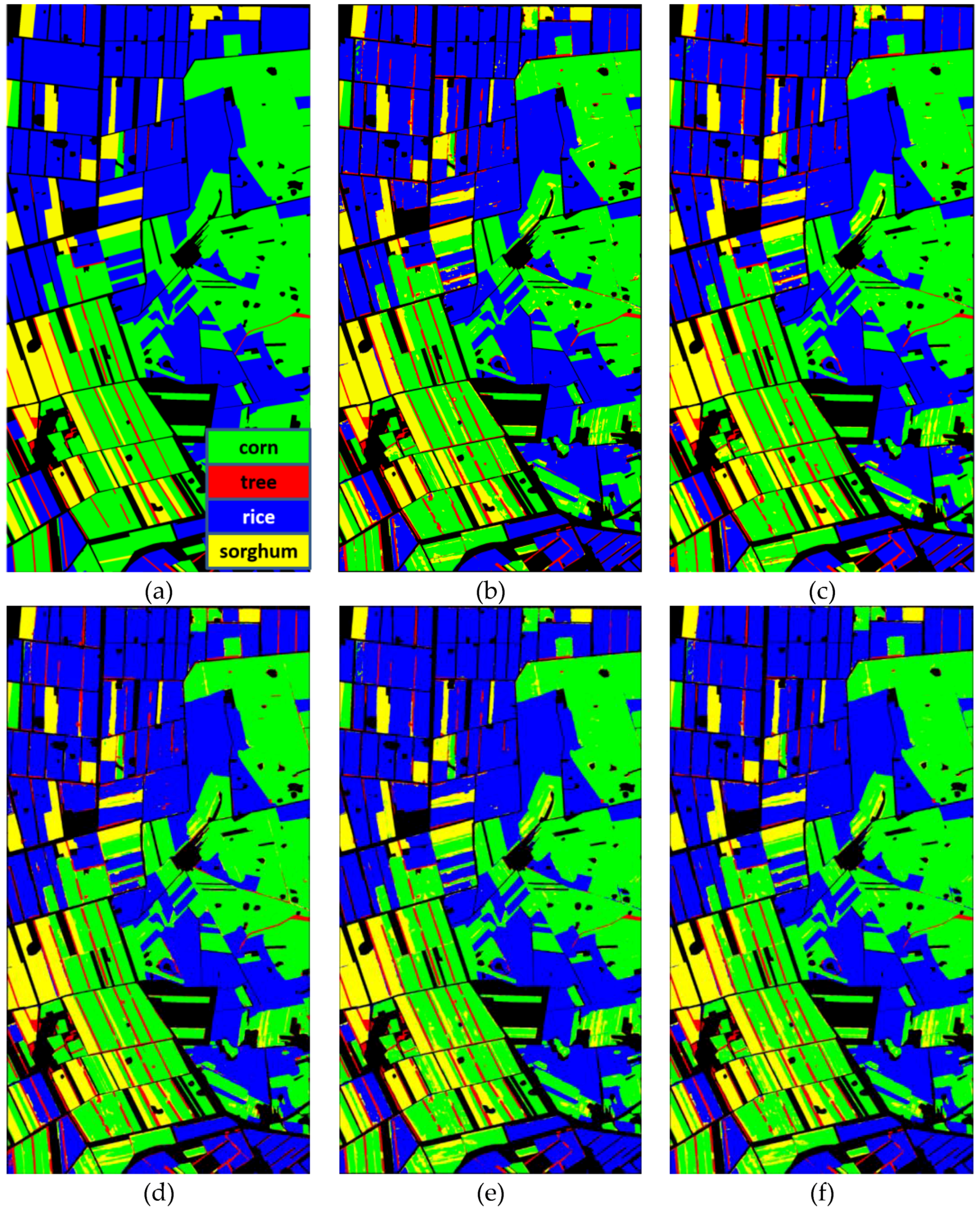
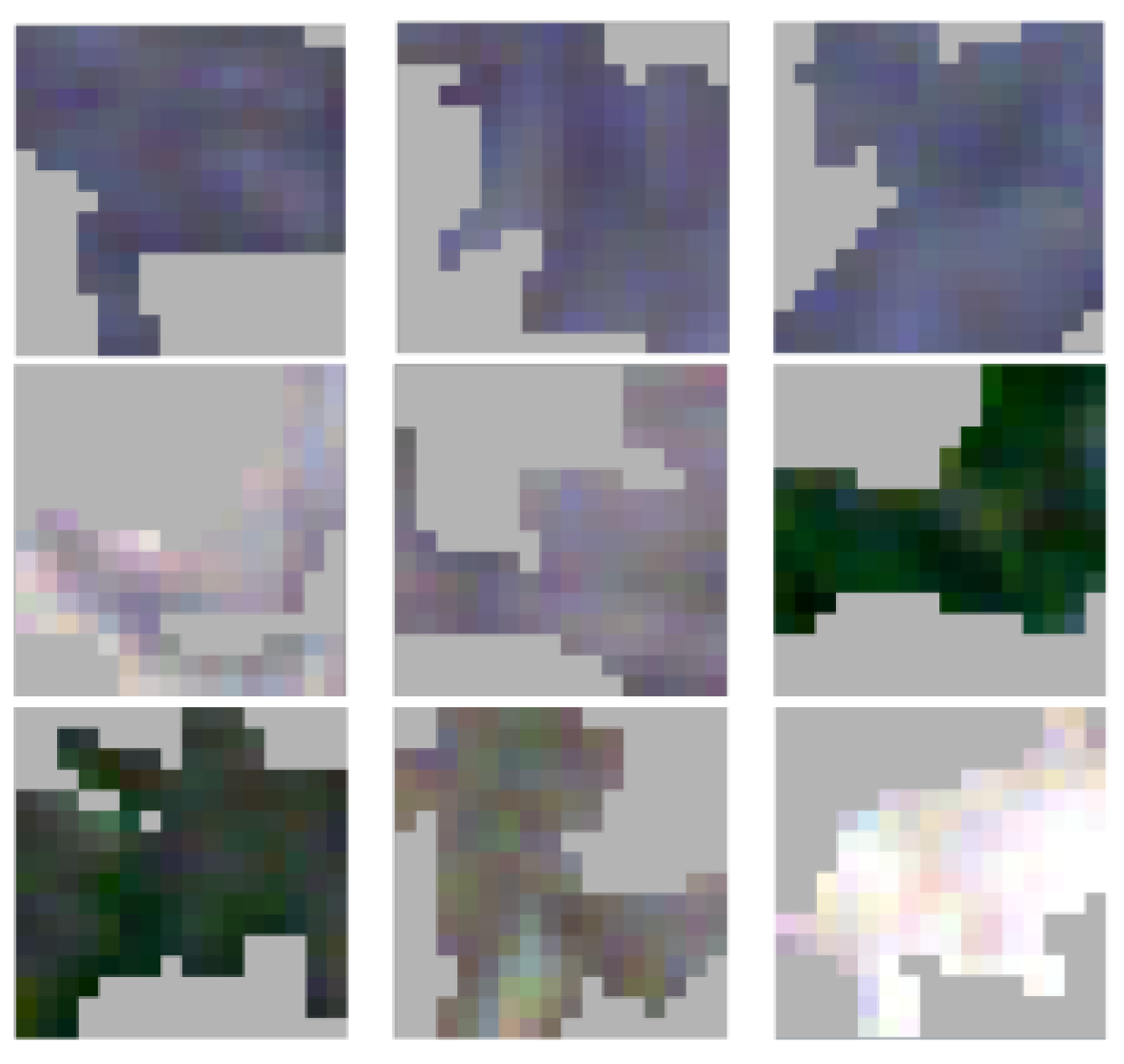
Except for CNN parameters, the quality of original samples is also important for remote sensing classification. A widely used preprocessing is segmenting original images to hyper-pixels for obtaining more “pure” samples. We test the performance of hyper-pixel inputs extracted from the GF1 data, when considering the 8 × 8 window patches we used before may contain mixed classes. The whole image is firstly segmented by the method that is developed by Liu et al. [39] to hyper-pixels, and every 8 × 8 patch sample (16 × 16 patch shown in Figure 11 instead for better vision) is then obtained by the superposition of the corresponding hyper-pixel upon 8 × 8 background template. However, the test accuracy decreased near 2 percent when compared to that of our original input. One plausible explanation is that the segmentation operation may introduce confusing information to classification, especially the shapes. The penalty of this exceeds the contribution of pixel purity. We did not test this on 3D CNN because the hyper-pixels containing the same sample points show different shapes in different periods.

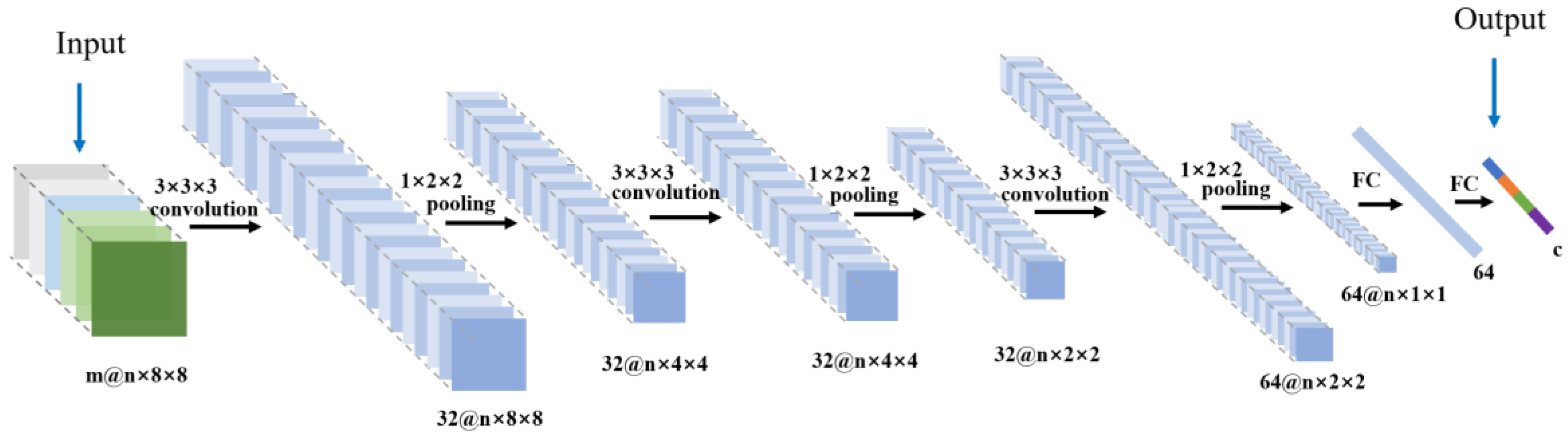
Another interesting question is whether spectral features, extracted from the combination of red, green, blue, and infrared bands, also have a high performance on crop classification. The current 3D convolutional network can be easily modified to check this by stacking the spectral images of a certain time first according to Figure 2. We applied the modified 3D tensor inputs on the GF1 dataset but kept all the CNN parameters the same. From

Table 7. 3D CNN results with spectrums as the third Dimension.

Data	Spatio-Spectral 3D CNN	2D CNN	Spatio-Temporal 3D CNN
GF1	0.760	0.772	0.794

, the spatio-spectral 3D CNN obtained much worse result when comparing to the spatio-temporal 3D CNN and a slightly worse result when comparing to the 2D CNN. The latter may be caused by the lack of more spectral bands or the inevitable noise in a “standard” spectral curve of a certain material, which is a common case in multi-spectral images. However, the processing of spatio-spectral information is not the focus of this study, and other recent articles could be referred [32].

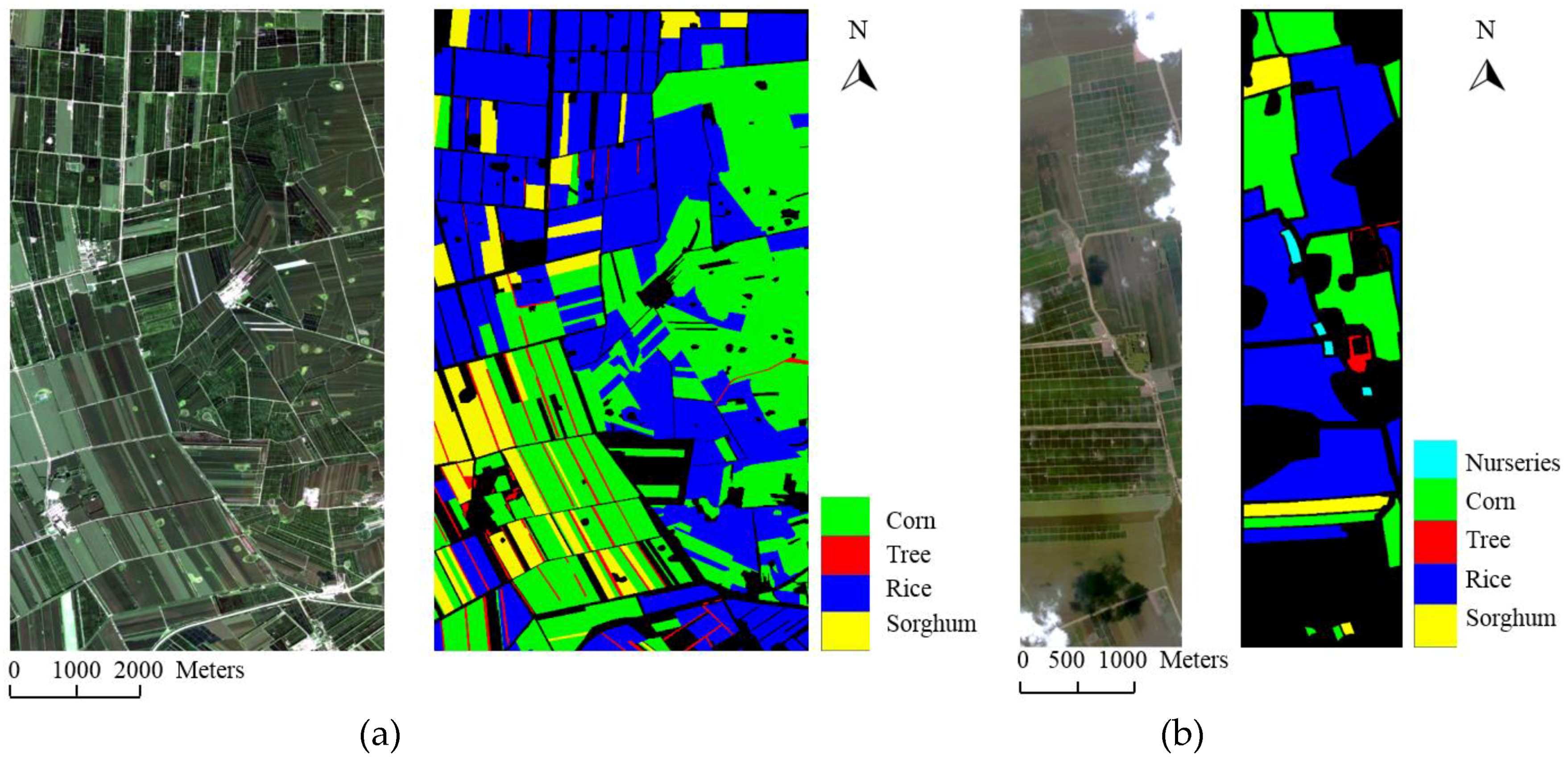
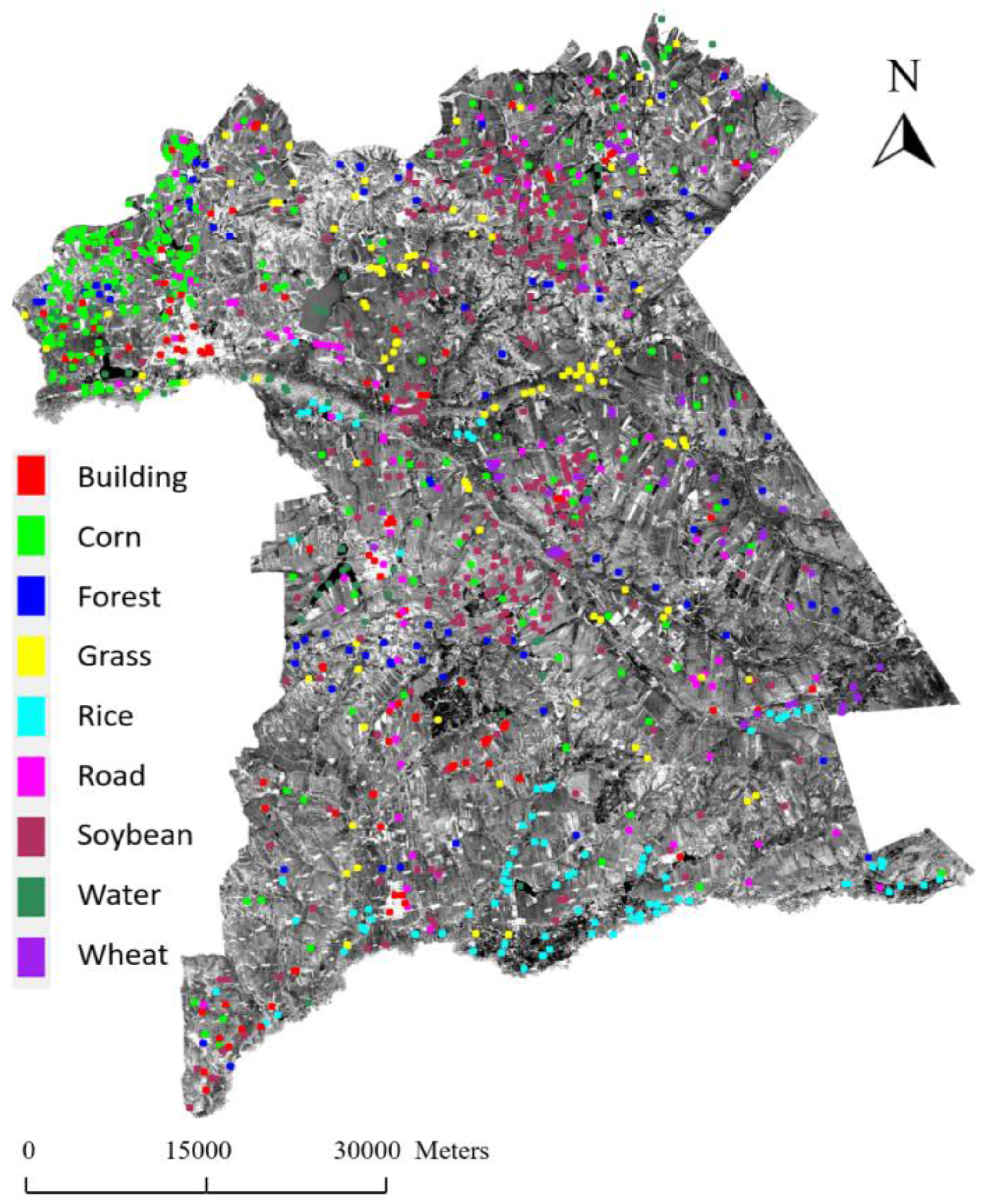
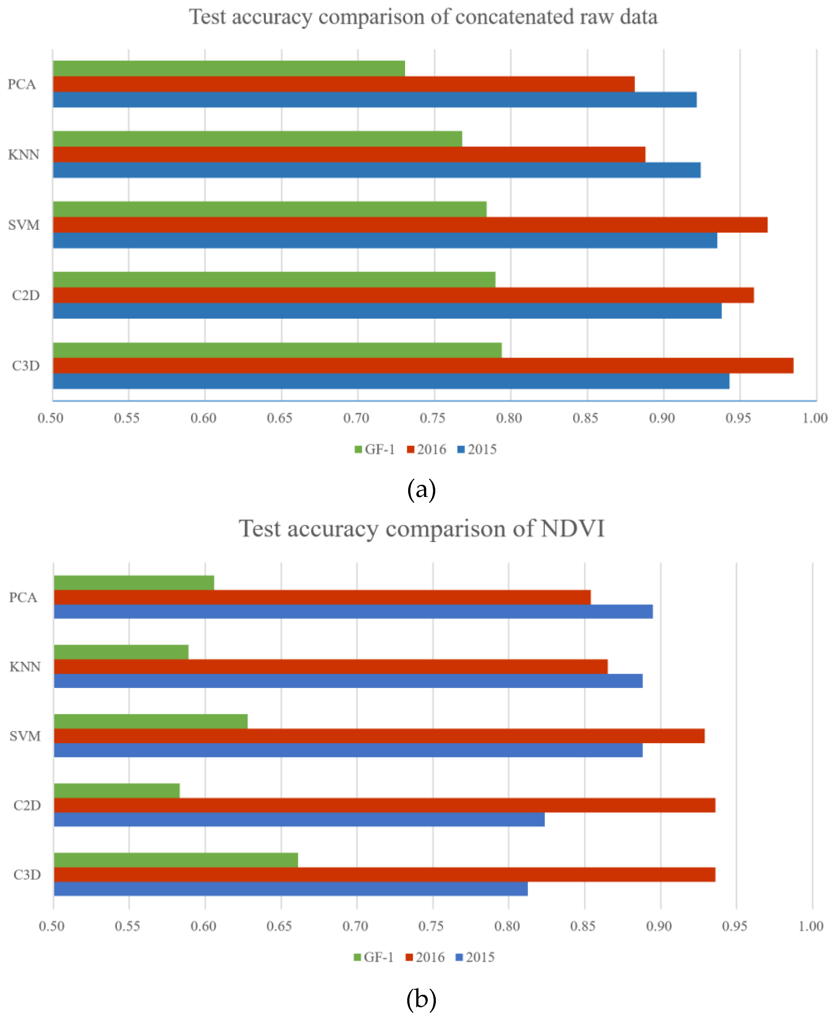
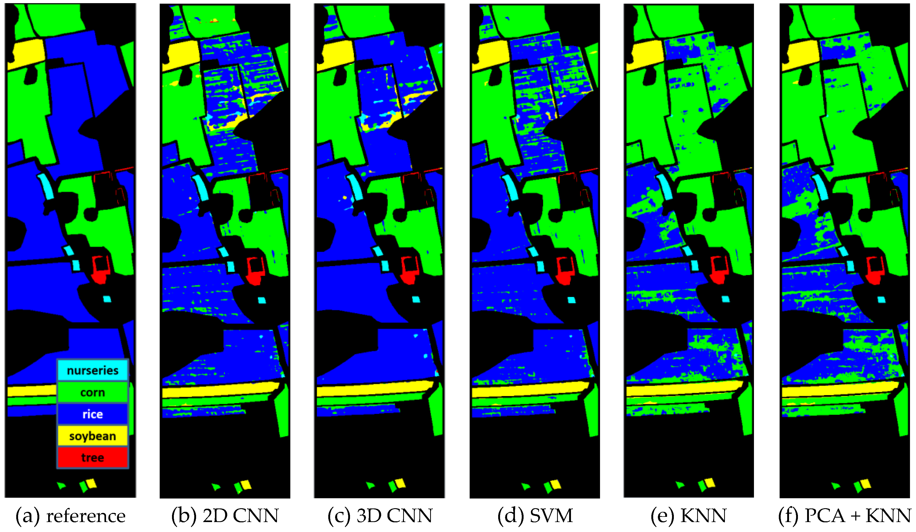
Third, we discuss more on the performance comparison of 2D CNN, 3D CNN, and SVM in pixelwise classification, which is the most common case in remote sensing applications other than the training-test procedure on discrete samples [8,12]. The overall accuracy of 3D CNN exceeds that of 2D CNN and SVM about 3% in average, and about 6% in the most challenging GF2 2016 data, where all of the other methods failed to discriminate corn from rice. The 3D CNN outperforms the 2D CNN purely with the learned spatio-temporal representations since they share the same parameters and classifier. The performance of SVM is approaching that of 2D CNN, which indicated that the concatenated temporal images are a good representation and match the state-of-the-art multi-level representation learned by a conventional CNN, if we ignore the classifier difference. It also explains from a side that the concatenated temporal images have been widely used in vegetation classification [12,13]. However, representing temporal features only by a concatenation operation is oversimplified and is not as good as spatio-temporal representations extracted by the 3D CNN.

At last, in this study, only temporal images and NDVI are used for feature inputs. We obtained similar result as Guerschman et al. [13], which also shows that advantage of using the whole spectral profile instead of the NDVI. The other method [8] utilized a feature combination of NDVI, humidity and luminance. Luminance is a spatial feature that could be extracted from original images, while humidity could be hard to accurately retrieve from spectral sensors with similar vegetarian covers. Testing all types of empirical features that are used before is unrealistic. We are interested in if additional empirical features could help the selectivity of CNN-based representations and further improve the performance of CNN methods. We added every NDVI layer to the corresponding original temporal image to train the 2D CNN.

Table 8. 2D CNN results with original images and the combination of original images and NDVI layers.

Data	Original	Original + NDVI
GF1	0.772	0.770

shows they obtained similar performances. It implies that a CNN based method could learn the optimal representations and including new empirical features is unnecessary.

5. Conclusions

Deep learning has been applied extensively in remote sensing applications. In this study, a novel method based on 3D CNN is introduced to crop classification using multi-temporal remote sensing images. The results show that the 3D CNN with proper structure performed better than either the conventional methods or the 2D CNN. According to the comparison of 2D and 3D CNN, 3D convolution could be a better feature extractor for spatio-temporal remote sensing data, while a common 2D convolution would lose the temporal information due to its own mathematical restriction, and a conventional method may take an oversimplified empirical rule to represent temporal features. In addition, we introduced an active learning strategy to CNN for improve the efficiency of manual labelling. It is very useful to embed the strategy in sample preparation or model refinement stage when the required accuracy is not achieved.

Furthermore, discovering the feasibility and efficiency of spatio-temporal feature representation by a 3D CNN could benefit not only in crop classification, but also other modelling process that is related to changes, trends or dynamics using remote sensing data. For example, embed a high-dimension deep learning framework into studies of glacier melting, climate changes, and seasonal forest dynamics, etc.

References

1. Wardlow, B.D.; Egbert, S.L.; Kastens, J.H. Analysis of time-series MODIS 250 m vegetation index data for crop classification in the US Central Great Plains. Remote Sens. Environ. 2007, 108, 2903–2910. [Google Scholar] [CrossRef]
2. Mathur, A.; Foody, G.M. Crop classification by support vector machine with intelligently selected training data for an operational application. Int. J. Remote Sens. 2008, 29, 2227–2240. [Google Scholar] [CrossRef]
3. Suykens, J.A.; Vandewalle, J. Least squares support vector machine classifiers. Neural Process. Lett. 1999, 9, 293–300. [Google Scholar] [CrossRef]
4. Blanzieri, E.; Melgani, F. Nearest neighbor classification of remote sensing images with the maximal margin principle. IEEE Trans. Geosci. Remote Sens. 2008, 46, 1804–1811. [Google Scholar] [CrossRef]
5. Murthy, C.; Raju, P.; Badrinath, K. Classification of wheat crop with multi-temporal images: Performance of maximum likelihood and artificial neural networks. Int. J. Remote Sens. 2003, 24, 4871–4890. [Google Scholar] [CrossRef]
6. Xiao, X.; Boles, S.; Liu, J.; Zhuang, D.; Frolking, S.; Li, C.; Salas, W.; Moore, B. Mapping paddy rice agriculture in southern China using multi-temporal MODIS images. Remote Sens. Environ. 2005, 95, 480–492. [Google Scholar] [CrossRef]
7. Conrad, C.; Colditz, R.; Dech, S.; Klein, D.; Vlek, P.G. Temporal segmentation of MODIS time series for improving crop classification in Central Asian irrigation systems. Int. J. Remote Sens. 2011, 32, 8763–8778. [Google Scholar] [CrossRef]
8. Sexton, J.O.; Urban, D.L.; Donohue, M.J.; Song, C. Long-term land cover dynamics by multi-temporal classification across the Landsat-5 record. Remote Sens. Environ. 2013, 128, 246–258. [Google Scholar] [CrossRef]
9. Simonneaux, V.; Duchemin, B.; Helson, D.; Er-Raki, S.; Olioso, A.; Chehbouni, A.G. The use of high-resolution image time series for crop classification and evapotranspiration estimate over an irrigated area in central Morocco. Int. J. Remote Sens. 2008, 29, 95–116. [Google Scholar] [CrossRef] [Green Version]
10. Conrad, C.; Fritsch, S.; Zeidler, J.; Rücker, G.; Dech, S. Per-field irrigated crop classification in arid Central Asia using SPOT and ASTER data. Remote Sens. 2010, 2, 1035–1056. [Google Scholar] [CrossRef] [Green Version]
11. Löw, F.; Michel, U.; Dech, S.; Conrad, C. Impact of feature selection on the accuracy and spatial uncertainty of per-field crop classification using support vector machines. ISPRS J. Photogramm. Remote Sens. 2013, 85, 102–119. [Google Scholar] [CrossRef]
12. Zhu, X.; Liu, D. Accurate mapping of forest types using dense seasonal Landsat time-series. ISPRS J. Photogramm. Remote Sens. 2014, 96, 1–11. [Google Scholar] [CrossRef]
13. Guerschman, J.; Paruelo, J.; Bella, C.D.; Giallorenzi, M.; Pacin, F. Land cover classification in the Argentine Pampas using multi-temporal Landsat TM data. Int. J. Remote Sens. 2003, 24, 3381–3402. [Google Scholar] [CrossRef]
14. Esch, T.; Metz, A.; Marconcini, M.; Keil, M. Combined use of multi-seasonal high and medium resolution satellite imagery for parcel-related mapping of cropland and grassland. Int. J. Appl. Earth Obs. Geoinf. 2014, 28, 230–237. [Google Scholar] [CrossRef]
15. Zhang, Y.; Wu, L. Crop classification by forward neural network with adaptive chaotic particle swarm optimization. Sensors 2011, 11, 4721–4743. [Google Scholar] [CrossRef] [PubMed]
16. Mcnairn, H.; Shang, J.; Jiao, X.; Champagne, C. The contribution of ALOS PALSAR multipolarization and polarimetric data to crop classification. IEEE Trans. Geosci. Remote Sens. 2009, 47, 3981–3992. [Google Scholar] [CrossRef]
17. Wang, H.; Zhang, J.; Xiang, K.; Liu, Y. Classification of remote sensing agricultural image by using artificial neural network. In Proceedings of the 2009 International Workshop on Intelligent Systems and Applications, Wuhan, China, 23–24 May 2009; pp. 1–4. [Google Scholar]
18. Tatsumi, K.; Yamashiki, Y.; Torres, M.C.; Taipe, C.R. Crop classification of upland fields using Random forest of time-series Landsat 7 ETM+ data. Comput. Electron. Agric. 2015, 115, 171–179. [Google Scholar] [CrossRef]
19. Omkar, S.N.; Senthilnath, J.; Mudigere, D.; Kumar, M.M. Crop classification using biologically-inspired techniques with high resolution satellite image. J. Indian Soc. Remote Sens. 2008, 36, 175–182. [Google Scholar] [CrossRef]
20. Gallego, J.; Kravchenko, A.; Kussul, N.; Skakun, S.; Shelestov, A.; Grypych, Y. Efficiency assessment of different approaches to crop classification based on satellite and ground observations. J. Autom. Inf. Sci. 2012, 44, 67–80. [Google Scholar] [CrossRef]
21. Siachalou, S.; Mallinis, G.; Tsakiristrati, M. A hidden markov models approach for crop classification: Linking crop phenology to time series of multi-sensor remote sensing data. Remote Sens. 2015, 7, 3633–3650. [Google Scholar] [CrossRef]
22. LeCun, Y.; Bengio, Y.; Hinton, G. Deep learning. Nature 2015, 521, 436–444. [Google Scholar] [CrossRef] [PubMed]
23. Cireşan, D.C.; Meier, U.; Gambardella, L.M.; Schmidhuber, J. Deep, big, simple neural nets for handwritten digit recognition. Neural Comput. 2010, 22, 3207–3220. [Google Scholar] [CrossRef] [PubMed]
24. Krizhevsky, A.; Sutskever, I.; Hinton, G.E. Imagenet classification with deep convolutional neural networks. In Proceedings of the 25th International Conference on Neural Information Processing Systems, Lake Tahoe, NV, USA, 3–6 December 2012; pp. 1097–1105. [Google Scholar]
25. Chen, Y.; Lin, Z.; Zhao, X.; Wang, G.; Gu, Y. Deep learning-based classification of hyperspectral data. IEEE J. Sel. Top. Appl. Earth Obs. Remote Sens. 2014, 7, 2094–2107. [Google Scholar] [CrossRef]
26. Mobahi, H.; Collobert, R.; Weston, J. Deep learning from temporal coherence in video. In Proceedings of the 26th Annual International Conference on Machine Learning, Montreal, QC, Canada, 14–18 June 2009; pp. 737–744. [Google Scholar]
27. Meszlényi, R.; Buza, K.; Vidnyánszky, Z. Resting state fMRI functional connectivity-based classification using a convolutional neural network architecture. Front. Neuroinform. arXiv 2017, arXiv:1707.06682. [Google Scholar]
28. Kussul, N.; Lavreniuk, M.; Skakun, S.; Shelestov, A. Deep learning classification of land cover and crop types using remote sensing data. IEEE Geosci. Remote Sens. Lett. 2017, 14, 778–782. [Google Scholar] [CrossRef]
29. Ji, S.; Xu, W.; Yang, M.; Yu, K. 3D convolutional neural networks for human action recognition. IEEE Trans. Pattern Anal. Mach. Intell. 2013, 35, 221–231. [Google Scholar] [CrossRef] [PubMed]
30. Tran, D.; Bourdev, L.; Fergus, R.; Torresani, L.; Paluri, M. Learning spatiotemporal features with 3D convolutional networks. In Proceedings of the 2015 IEEE International Conference on Computer Vision, Santiago, Chile, 7–13 December 2015; pp. 4489–4497. [Google Scholar]
31. Maturana, D.; Scherer, S. 3D convolutional neural networks for landing zone detection from lidar. In Proceedings of the 2015 IEEE International Conference on Robotics and Automation (ICRA), Seattle, WA, USA, 26–30 May 2015; pp. 3471–3478. [Google Scholar]
32. Li, Y.; Zhang, H.; Shen, Q. Spectral-spatial classification of hyperspectral imagery with 3D convolutional neural network. Remote Sens. 2017, 9, 67. [Google Scholar] [CrossRef]
33. Tong, S.; Koller, D. Support vector machine active learning with applications to text classification. J. Mach. Learn. Res. 2001, 2, 45–66. [Google Scholar]
34. Dahl, G.E.; Sainath, T.N.; Hinton, G.E. Improving deep neural networks for LVCSR using rectified linear units and dropout. In Proceedings of the 2013 IEEE International Conference on Acoustics, Speech and Signal Processing (ICASSP), Vancouver, BC, Canada, 26–31 May 2013; pp. 8609–8613. [Google Scholar]
35. Simonyan, K.; Zisserman, A. Very deep convolutional networks for large-scale image recognition. Available online: http://adsabs.harvard.edu/abs/2014arXiv1409.1556S (accessed on 5 January 2018).
36. Goodfellow, I.; Bengio, Y.; Courville, A. Deep Learning; MIT Press: Cambridge, MA, USA, 2016. [Google Scholar]
37. Bernstein, L.S.; Adlergolden, S.M.; Sundberg, R.L.; Levine, R.Y.; Perkins, T.C.; Berk, A.; Ratkowski, A.J.; Felde, G.; Hoke, M.L. Validation of the QUick atmospheric correction (QUAC) algorithm for VNIR-SWIR multi- and hyperspectral imagery. Proc. SPIE 2005, 5806, 668–678. [Google Scholar]
38. Jolie, I. Principal Component Analysis; Springer: New York, NY, USA, 1986. [Google Scholar]
39. Liu, M.-Y.; Tuzel, O.; Ramalingam, S.; Chellappa, R. Entropy rate superpixel segmentation. In Proceedings of the 2011 IEEE Conference on Computer Vision and Pattern Recognition (CVPR), Colorado Springs, CO, USA, 20–25 June 2011; pp. 2097–2104. [Google Scholar]
Figure 1. Comparison of two-dimensional (2D) and three-dimensional (3D) convolution. The image patches of the same area are captured in May, June, July, September and October. In (a) 2D convolution, ⊗2 indicates 2D convolution operator where no relations exist between extracted features (in different color) in temporal direction; ⊕ is sum operator where all features are collapsed. In (b) 3D convolution, ⊗3 indicates 3D convolution operator with length 3 in temporal direction. The operator is executed three times sequentially (in red, green and blue arrows) through temporal direction. The features pointed by the same-color arrows then contain temporal information, and output map is also a 3D tensor.
Remotesensing 10 00075 g001
Figure 2. 3D convolution strategy for multi-temporal multi-spectral image input in this study. A 3D feature map is obtained after 3D convolution on spatio-temporal images and accumulating over different spectral bands (denoted by different border colors).
Remotesensing 10 00075 g002
Figure 3. The network structure of 3D convolutional neural network (CNN) for multi-temporal crop classification.
Remotesensing 10 00075 g003
Figure 4. The network structure of 2D CNN for multi-temporal crop classification.
Remotesensing 10 00075 g004
Figure 5. GF2 images captured in (a) 2015 and (b) 2016, respectively. Black pixels in the shape files are lack of label information.
Remotesensing 10 00075 g005
Figure 6. The GF1 testing data.
Remotesensing 10 00075 g006
Figure 7. Test accuracy (red line), training loss (blue line), and test loss (green line) with optimal parameters. The test accuracy of 3D CNN shows 0.7%, 1.7% and 2.2% higher than that of 2D CNN in GF2-2015, GF2-2016 and GF1 data, respectively. (a) 3D CNN for GF2 2015 data; (b) 2D CNN for GF2 2015 data; (c) 3D CNN for GF2 2016 data; (d) 2D CNN for GF2 2016 data; (e) 3D CNN for GF1 data; and, (f) 2D CNN for GF1 data.
Remotesensing 10 00075 g007aRemotesensing 10 00075 g007b
Figure 8. Comparison of test accuracy among 2D CNN, 3D CNN, SVM, KNN, and PCA with NDVI and original data respectively. (a) Concatenated temporal image patches as input; (b) Concatenated NDVI maps of different periods as input.
Remotesensing 10 00075 g008
Figure 9. Pixelwise classification results of different methods on GF2 2015 data. (a) reference; (b) 2D CNN; (c) 3D CNN; (d) SVM; (e) KNN; and, (f) PCA + KNN.
Remotesensing 10 00075 g009
Figure 10. Pixelwise classification results of different methods on GF2 2016 data. (a) reference; (b) 2D CNN; (c) 3D CNN; (d) SVM; (e) KNN; and, (f) PCA + KNN.
Remotesensing 10 00075 g010
Figure 11. Hyper-pixel inputs.
Remotesensing 10 00075 g011