Issues with Large Area Thematic Accuracy Assessment for Mapping Cropland Extent: A Tale of Three Continents

Abstract

Accurate, consistent and timely cropland information over large areas is critical to solve food security issues. To predict and respond to food insecurity, global cropland products are readily available from coarse and medium spatial resolution earth observation data. However, while the use of satellite imagery has great potential to identify cropland areas and their specific types, the full potential of this imagery has yet to be realized due to variability of croplands in different regions. Despite recent calls for statistically robust and transparent accuracy assessment, more attention regarding the accuracy assessment of large area cropland maps is still needed. To conduct a valid assessment of cropland maps, different strategies, issues and constraints need to be addressed depending upon various conditions present in each continent. This study specifically focused on dealing with some specific issues encountered when assessing the cropland extent of North America (confined to the United States), Africa and Australia. The process of accuracy assessment was performed using a simple random sampling design employed within defined strata (i.e., Agro-Ecological Zones (AEZ’s) for the US and Africa and a buffer zone approach around the cropland areas of Australia. Continent-specific sample analysis was performed to ensure that an appropriate reference data set was used to generate a valid error matrix indicative of the actual cropland proportion. Each accuracy assessment was performed within the homogenous regions (i.e., strata) of different continents using different sources of reference data to produce rigorous and valid accuracy results. The results indicate that continent-specific modified assessments performed for the three selected continents demonstrate that the accuracy assessment can be easily accomplished for a large area such as the US that has extensive availability of reference data while more modifications were needed in the sampling design for other continents that had little to no reference data and other constraints. Each continent provided its own unique challenges and opportunities. Therefore, this paper describes a tale of these three continents providing recommendations to adapt accuracy assessment strategies and methodologies for validating global cropland extent maps.

1. Introduction

Accurate and consistent cropland information is crucial to answer the issues of global food security to make future policy, investment and logistical decisions [1,2,3,4,5,6,7]. Global cropland mapping provides baseline cropland information to accurately assess the drivers and implications of cropland dynamics both at regional and global scale [8,9,10]. To predict and respond to food insecurity, global cropland products are readily available from coarse and medium spatial resolution earth observation data. Therefore, remote sensing has been recognized as an extremely effective, economical and feasible approach to create cropland thematic maps over a range of spatial and temporal scales [11,12,13].

Cropland maps such as Global Map of Irrigation Areas (GMIA), Global Map of Rain-fed Areas (GMRCA) [14], Global Monthly Irrigated and Rain-fed Crop Areas (MIRCA2000) [15], Global Rain-fed, Irrigated and Paddy Croplands (GRIPC) [16] and MODIS-Cropland [17] derived from coarse-resolution satellite data are currently some of the main sources of cropland information on a global scale. However, these types of products either have insufficient accuracy or their resolution is too coarse for use in other than global applications [10]. More recently, with advances in remotely sensed imagery and classification algorithms implemented on cloud computing platforms such as Google Earth Engine, cropland products are available at higher spatial resolutions. For example, global cropland products were generated at 250 m and 30 m spatial resolutions by the NASA MEaSURES (Making Earth System Data Records for Use in Research Environments) GFSAD (Global Food Security Data Analysis) project [18,19,20,21].

Previously, accuracy assessments performed on most global cropland extent maps were conducted to produce a single global accuracy measure (i.e., overall accuracy) without regard to continental or regional differences [22,23]. These measures could then be used to make a statement about the overall accuracy of the global map, but not about specific continents or regions [24]. The accuracy of a specific continent or region could only be determined if an assessment was done for that area. Insufficient availability of reference data in most regions of the world along with significant variations in agricultural landscape patterns offers unique challenges to conduct a more detailed accuracy assessment of any global mapping product. The reference data required to perform the assessment over large area cropland maps are not uniformly available for all the continents. For instance, some of the continents have extensive reference data available for assessment (such as US and Canada) while other continents (such as Africa) have very little to none. Additionally, mapping in some continents exhibits larger errors than others simply depending on the complexity of the agriculture landscapes [25,26]. For example, it has been reported that an accurate map is difficult to achieve in developing countries with small holder agricultural landscape by the International Food Policy Research Institute (IFPRI) [27]. Therefore, most of the global assessments have not attempted to provide a more regionalized measure of accuracy encompassing continents/regions or different agriculture landscapes [28].

Clearly, a single accuracy estimate will not provide a holistic view of the ability to map variation within the agriculture landscapes of different continents. However, these continental variations could be reported by assessing the map accuracy in response to different issues observed in the cropland maps of different continents [22,29,30,31]. Therefore, a continent-based assessment strategy will provide more intensive evaluation of the cropland maps in agriculture landscapes for different continents. This kind of intense and efficient assessment strategy for different continents will also help to understand the efficacy, quality and variations of large area cropland maps [32]. Therefore, the question is how to implement such a continent-based assessment strategy effectively for each continent while also considering the different kinds of issues and constraints related to both reference data availability and complexity of agriculture landscapes.

While individual measures of accuracy are well established in literature (e.g., [30,31,33]), considerable ambiguity remains about the implementation and interpretation of accuracy assessment for large areas. The most widely accepted approach to perform an accuracy assessment is through the use of an error matrix [31]. The error matrix is a cross tabulation of the class labels predicted by the image classification against that observed from the reference dataset. The key issue in generating a valid error matrix is the collection of sufficient and appropriate reference data. The collection of such data must be conducted using an appropriate sampling scheme with sufficient samples in consideration of the complexities of the area being mapped [24].

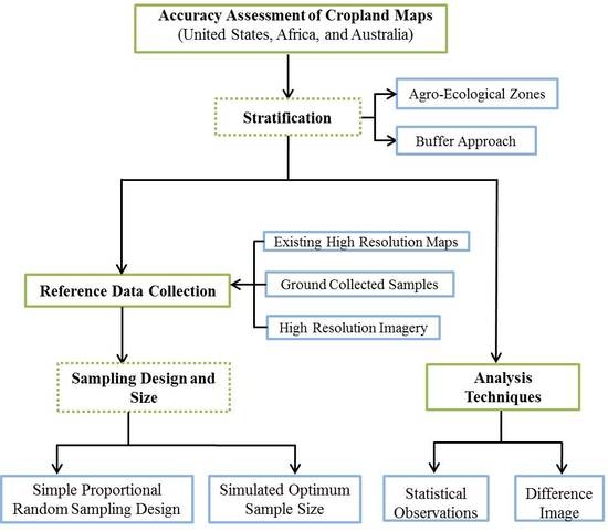
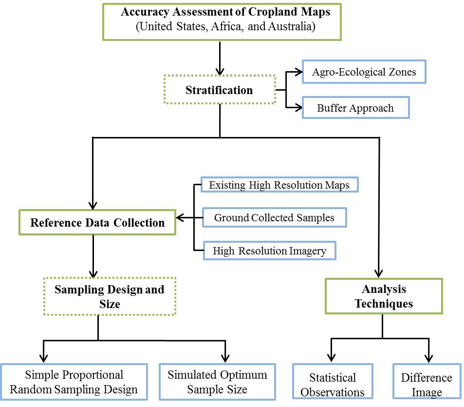
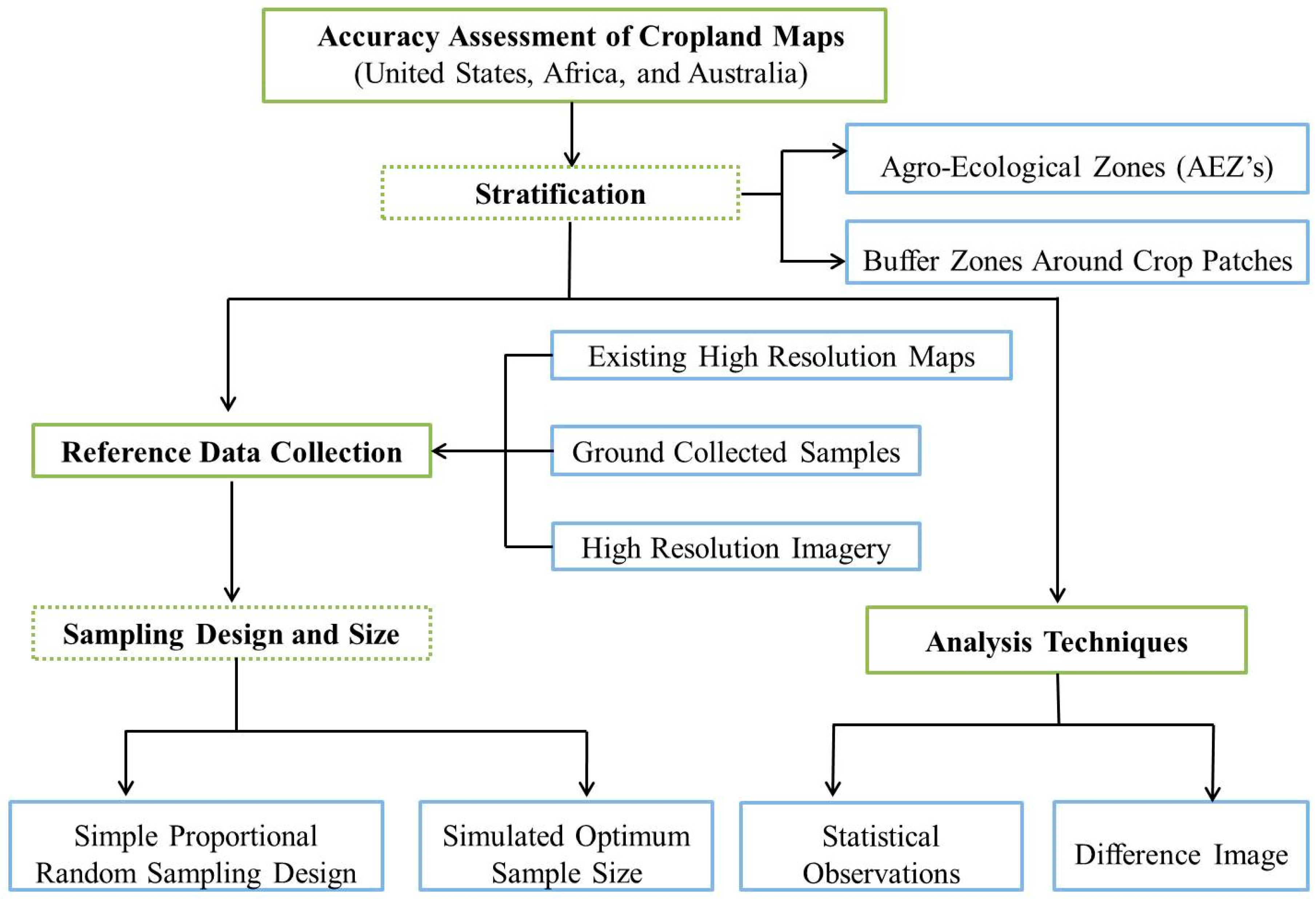
In order to conduct a detailed continent-based assessment of cropland extent maps generated in the GFSAD project, it was important to consider how the mapping was performed in each continent. The cropland extent maps for each continent were created by dividing the area into homogeneous regions (i.e., stratification) rather than just producing a single map of the entire continent. As a result, the accuracy assessment was also performed within these homogeneous areas using traditional assessment methods with modified sampling designs for collecting reference data depending on the agriculture landscapes in each continent [23,30]. Such modified sampling designs for collecting reference data ensured an optimum sampling approach considering different agriculture landscapes in each continent. Therefore, continent-based accuracy assessment of the cropland maps generated in GFSAD project was conducted by continent in response to different issues and constraints observed in the cropland extent maps.

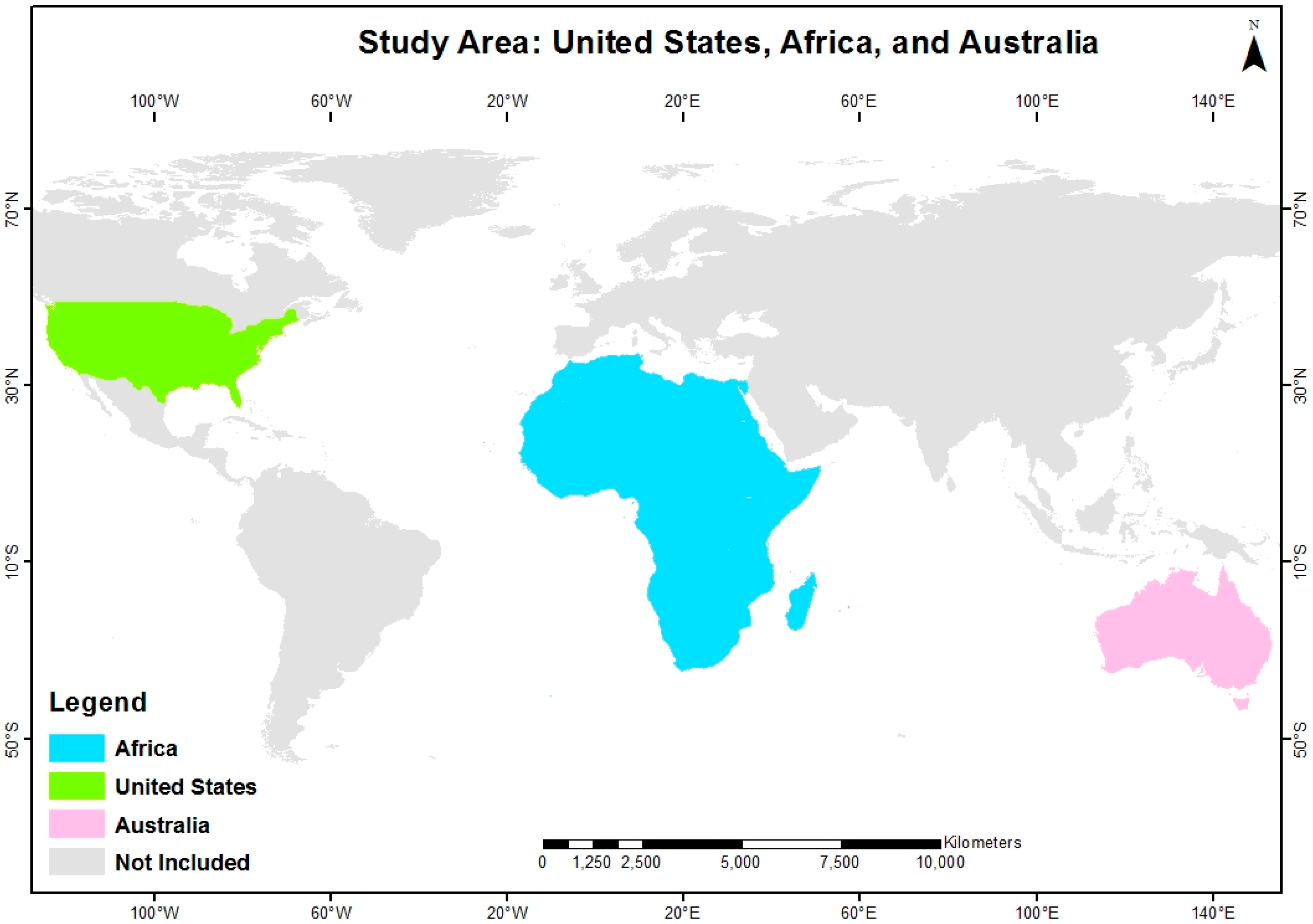
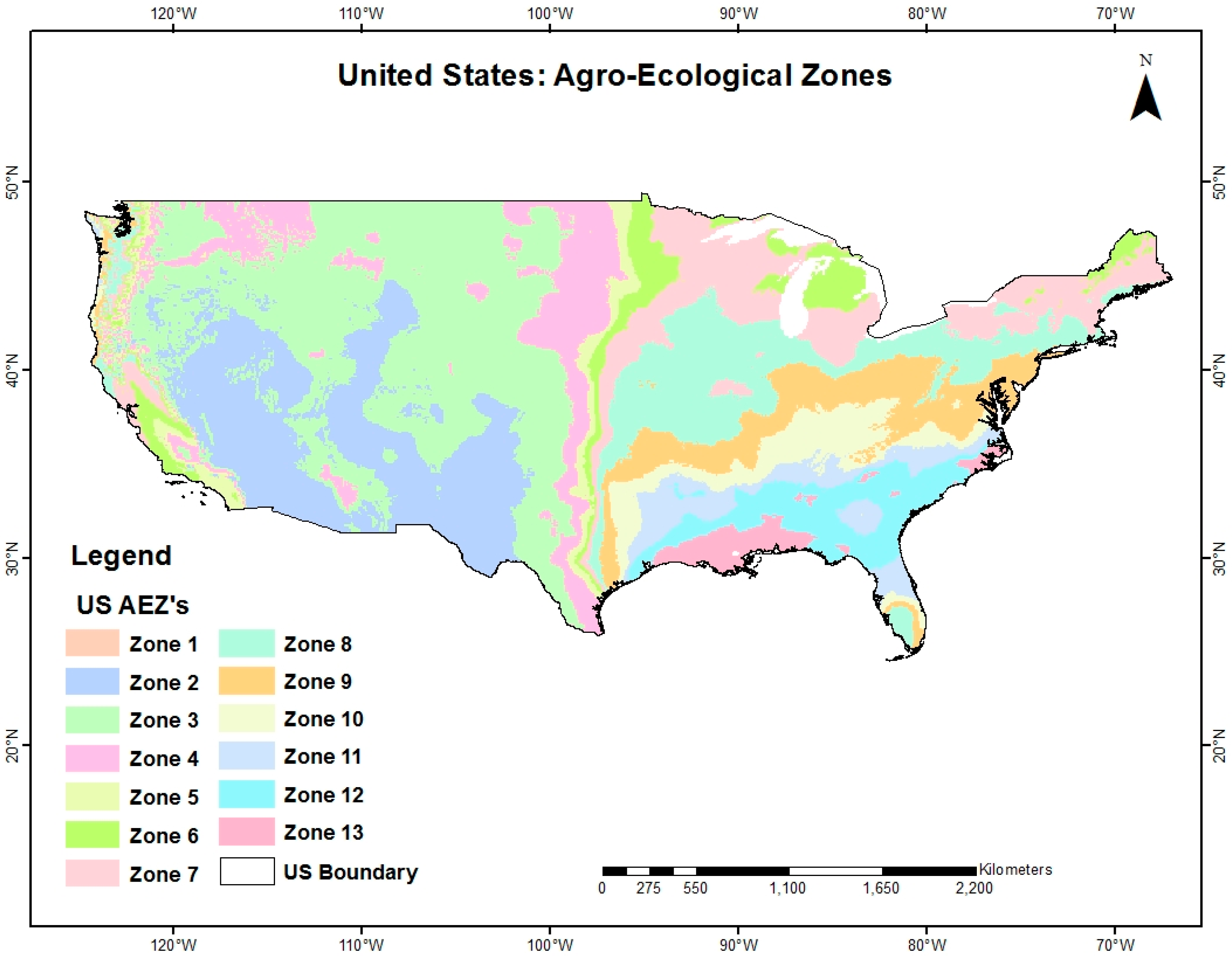
The goal of this paper is to provide specific approaches and recommendations for modifying existing accuracy assessment strategies and methodologies to validate global cropland extent maps considering the issues and constraints unique to each continent. Meaningful and statistically valid assessment results demonstrate that these methods and approaches contribute a better understanding of global cropland distribution by continent. This work is specifically focused on dealing with unique issues encountered when assessing cropland extent for North America (confined to the USA), Africa and Australia. These three continents were selected as a representative of different cropping patterns with variable size agriculture fields and availability of reference data. Lessons learned from this work can be further extended to other continents to provide appropriate methods of accuracy assessment where different scenarios of reference data availability and agriculture landscapes exist. The approach of stratifying the continents based on Agro-Ecological Zones (AEZ’s) for the US and Africa provided rigorous and valid accuracy results [29]. The buffer-based stratification approach used in Australia also provides an alternative methodology for when crops are clustered only in certain areas of the continent and are not appropriately represented by AEZ’s.

2. Materials and Methods

This section describes the study area and the generalized methodology used for assessing the cropland maps of three continents selected throughout the world. The results then detail how these generalized methods were implemented to deal with specific issues and constraints found in each continent.

2.1. Study Area

The study area for this paper includes three continents (i.e., North America (confined to United States), Africa and Australia) where a wide variety of climate, topography, moisture and crop growing periods prevail due to the large size, range of geographic features and non-contiguous arrangement of homogeneous agriculture landscapes [34] (Figure 1). For North America, the United States (US) was chosen as a representative of the continent. This assumption is appropriate here as the issues and constraints found in the US also hold for Canada and Mexico. For the other two continents, the entire continent has been assessed. Food and Agriculture Organization (FAO) Agro-Ecological Zones (AEZ’s) that are defined by the length of the growing period days derived from temperature, precipitation and soil water holding capacity were used to stratify both the US and Africa [35]. Both the mapping and the accuracy assessment were performed within these homogeneous areas (AEZ’s). However, this AEZ-based stratification method resulted in more fragmented zones when applied to Australia because of a single, large area in the center of the continent having low probability of cropland. Therefore, a different and more effective stratification method (i.e., buffering approach) was used instead to define an appropriate sampling area around the cropland patches for the Australian continent.

The US is composed mostly of large, agriculturally homogeneous regions and large area farming is prevalent due to abundant land availability [34]. The cropland areas are roughly concentrated in the central regions of the US; pastures are in the more arid west; and forest land in the East, where the topography and precipitation patterns are conducive to growing trees (USDA, Economic Research, 2012). Dominant crops such as corn and soybeans are grown in large, homogeneous, agriculture fields. In contrast, there are some heterogeneous regions in the US that grow rare crops and have a high diversity of crop types. All of these crop areas along with their specific types have been regularly mapped by USDA-NASS (i.e., United States Department of Agriculture-National Agricultural Statistics Service) every year since 2009 for all 48 conterminous states with a 30 m pixel resolution [36]. Before 2009, cropland was mapped at 56 m spatial resolution. All these data are readily available in a database called the Cropland Database Layer (CDL) and can be used as reference data for other mapping efforts including the GFSAD project. Therefore, in the US, assessing cropland maps is much easier than any other part of the world.

Africa has more scattered cropland distribution than any other cropping region of the world. The variation between AEZ’s in Africa is large, ranging from the dry and barren desert, through the rich soil of the Rift, Nile and Niger River Valleys, to the southern extremes. However, unlike any other parts of the world, there are no large crop belts in Africa. Rather, there are agricultural regions within which different combinations of crops are cultivated [34].

Australia closely resembles other temperate regions of the world. Wheat is the dominant crop in Australia; it is interrupted only briefly by a combination of wheat and barley in the southern part of the continent. In the western portion of the Australian Wheat Belt, pulses are the most prominent secondary crop, while barley is the secondary crop in the eastern portions. Pulses are the third most dominant crop (about 11%) [37]. However, the total cropland distribution is restricted to a ring-like region around the edges of the continent. Therefore, to minimize cropland omission and commission errors and to avoid sampling where there was no possibility of finding a crop, the area surrounding the crop patches was chosen for sampling through the use of a buffering approach instead of using AEZ’s.

2.2. Methods

The typical approach to perform a statistically rigorous thematic accuracy assessment of any map generated from remotely sensed imagery includes collecting reference data and then computing descriptive statistics [31]. This paper focuses on the accuracy assessment of large area cropland extent maps generated for the entire world. The methods to perform such an accuracy assessment must include the consideration of specific issues, concerns and characteristics for each continent including: (1) the appropriate stratification; (2) the effective and valid collection of reference data; (3) the appropriate sampling; and (4) the application of a descriptive analysis protocol (Figure 2).

2.2.1. Stratification

Continents with diverse cropping patterns are expected to have variations in classification accuracy due to a number of reasons including: these diverse cropping patterns, differences in the classifiers employed to create the maps and the different spatial resolutions of the satellite images used [37,38]. It is more likely that low accuracy and confidence levels are achieved in mapping rare classes due to their limited population size [39]. When comparing the cropland maps of different continents, it has been shown that high agreement and consistency in accuracy is associated with areas of no or almost fully covered agricultural classes [40]. However, the regions with scattered and sparse cropping patterns contained more uncertainty and inconsistency. The issue of variations in different agriculture landscapes must be considered and addressed by modifications to the accuracy assessment strategy. The assessment of cropland maps and reporting the accuracy estimates for homogeneous regions of similar cropping patterns using some type of stratification approach will result in more meaningful, representative and applicable mapping products [39].

There are two advantages of implementing a stratification method while mapping cropland areas and assessing their accuracy. First, implementing a stratification method of dividing a large mapping area into homogeneous regions reduces the extent of the area to be mapped and assessed. The stratification then results in more efficient performance of the classification algorithm in response to the variations of each region and allows for more effective validation [40]. Secondly, the stratification method also helps to optimize the efforts required to collect a valid and efficient reference dataset required for mapping and assessing the accuracy of the cropland areas [41]. The choice of an appropriate stratification method could be either based on the mapped classes or homogeneous zones of different cropping and climatic conditions such as Agro-Ecological Zones (AEZ’s) in any particular area of interest (i.e., a continent).

AEZ-based stratification methods were used to divide the study area into more homogeneous regions in previous research such as simulating crop yield potentials [42], global change assessment the [43] and climate change [44] projects. Therefore, AEZ-based stratification method will also help to divide different continents into homogeneous regions to implement the assessment strategy required to assess the cropland extent maps [45]. However, it is difficult to divide sparse cropland regions into homogeneous zones based on AEZ’s. In such sparse cropland regions, AEZ-based stratification methods result in more fragmented zones rather than homogeneous ones. Therefore, a more representative stratification method is required to define an appropriate sampling area around the sparse cropland patches (for example, Australia). Upon close examination of the cropland distribution in the three selected continents (i.e., US, Africa and Australia), two stratification methods (i.e., AEZ’s and Euclidean distance buffering) were used to divide the continents into zones before assessing the cropland maps. In US and Africa, the cropland extent was stratified using the AEZ approach based on the number of growing period days. In Australia, the cropland distribution is mostly concentrated in a narrow belt towards the edges of the continent leaving a large portion toward the center with a very low likelihood of crops. Therefore, a buffering approach rather that an AEZ approach was used for stratification in Australia.

2.2.2. Collecting Reference Data

The reference data can be sourced either from ground-collected data, or from any existing appropriate reference maps (e.g., USDA CDL), or from interpretation of very high-resolution imagery (VHRI). However, in many cases, a difference in the classification scheme between the existing reference data and the map to be assessed and/or the size of the sample unit (often too small) can limit the use of any existing reference data [46,47]. Therefore, ground collected data are considered as the optimal, yet most expensive, reference data. The timing of the reference data collection for assessing agricultural maps is also a very important factor. Significant errors can occur when not keeping the reference data collection to as near as possible to the image collection date [24]. It is critical that the reference data be independent of any other data used for training and initial testing of the thematic mapping. Once the independency, timing and source of the reference data are achieved, it is important to choose the appropriate sampling design and sample size.

Upon completion of a thorough search for any readily available reference data for the three continents, an independent source of reference data was generated using an appropriate sampling design in the homogeneous regions for each continent. For example, existing reference maps (e.g., CDL for the US with an accuracy range of 85–95% [36]) can be used as reference data to perform the assessment of cropland extent map while ground sampling or interpretation of very high-resolution imagery (VHRI) might be performed for continents such as Africa with little to no existing reference data. In addition, a field campaign (i.e., ground sampling) usually focuses on collecting the reference data for the map class of interest (in our case, crops). Therefore, to generate a proportionally balanced reference dataset, additional reference samples may need to be interpreted from VHRI. In this study, a combination of the three different sources of reference data (i.e., existing reference maps, independent generated random samples and ground collected samples) were ultimately used to assess the cropland extent maps of the three selected continents.

2.2.3. Sampling

Many researchers have published suggestions regarding the proper sampling scheme to use for collecting reference data depending on different regions of interest (e.g., [48,49,50]). These suggestions vary from simple random sampling to stratified, systematic and other sampling approaches for assessing the accuracy of remotely sensed maps. There are both pros and cons associated with each of these types of sampling schemes. Another study [51] has proposed the relative strengths and weakness of these different sampling designs based on seven desirable criteria. These criteria are: (1) probability-based; (2) practical implications; (3) cost effectiveness, (4) spatially balanced; (5) precise estimates of class-specific accuracy; (6) ability to estimate standard errors; and (7) flexibility to change the sample size.

Systematic and spatially stratified designs were generally rated as strong on the spatially balanced criterion, whereas the designs stratified by thematic map classes were strong for determining class-specific accuracy. Systematic sampling was usually rated as weak due to non-availability of an unbiased variance estimator. A key issue in sampling is that of randomness such that each sample (in this case, crop and no-crop) has an equal and independent chance of being selected [24]. Given that in this project there were only two map classes, simple random (probability-based) sampling with flexibility to modify the sample size for each continent is the best scheme. Therefore, a simple random sampling design was selected to distribute samples in different agriculture landscapes of the three selected continents to assess the accuracy of the cropland maps.

Once the sampling scheme was selected, then the next question is to decide the size of the sample unit. In literature, a cluster of pixels has been suggested to be used as the sample unit when assessing the accuracy of cropland maps derived from medium resolution imagery. Selecting a homogeneous cluster of 3 × 3 pixels accounts for issues in positional accuracy for maps derived from 30 m or so satellite imagery to ensure that thematic accuracy is being analyzed and not positional error [24]. However, it is extremely difficult to find a 3 × 3 homogeneous cluster of pixels for coarse resolution satellite imagery (250 m pixels). Therefore, a single pixel sample unit was used to collect reference samples to assess the accuracy of the 250 m cropland maps in the three selected continents.

The most challenging component of assessing the accuracy of a thematic map is collecting enough samples to perform a valid assessment. Different equations and guidelines have been established by many researchers for choosing an appropriate sample size [48,49,52,53,54,55]. In the literature, a method based on Monte Carlo simulation [53] suggested that most thematic maps can be assessed using a sample size of 50 for each mapped class. However, given that the areas to be assessed here (AEZ or buffer zones) are quite large, a sample simulation using the Monte Carlo method was performed to determine the appropriate sample size. Based on the results of the sample simulation, an appropriate sample size was selected for each of the selected continent.

2.2.4. Computing Descriptive Statistics

The last step in an accuracy assessment is the descriptive analysis protocol to report accuracy measures in the form of an error matrix and, in some cases, spatial agreement and disagreement analysis using a difference image. Once an error matrix has been properly generated, it can be used as a starting point to calculate individual class accuracies (i.e., producer’s and user’s accuracies) in addition to an overall accuracy [56]. The producer’s and user’s accuracy are often called commission and omission errors, respectively. A commission error is defined as including an area into a thematic class when it does not belong to that class while an omission error is excluding that area from the thematic map when it belongs to the map. Omission errors can be calculated by dividing the total number of correctly classified sample units in a category by the total number of sample units in that category from the reference data [31,56]. Commission errors, on the other hand, are calculated by dividing the number of correctly classified sample units for a category by the total number of sample units that were classified in that category [30,31,56].

In addition to these statistical measures, a difference image can also be created by comparing the map with an existing cropland map created by other researchers for each continent and spatially depicting the agreement and disagreement in the map classes. This image can only be generated when there is another thematic map available such as in the US, where reference data sets are available that cover the entire study area. In most areas of the world, these reference maps do not exist and only limited reference data samples are available.

When the reference map is assumed to be 100% correct, the difference image is used to depict the omission and commission errors that occurred between the two cropland maps. Unless the comparison is being conducted using a reference map, the different image demonstrates similarity between the two maps rather than an omission and commission error. Once the difference image is created, the results can also be shown in a similarity matrix, which is generated in the same way as an error matrix.

3. Results

The results of the accuracy assessment process that was performed including specific issues and constraints observed in the cropland maps are presented in the following three major components for each of the three selected continents: (1) Stratification: dividing each continent into homogeneous regions; (2) Collecting reference data and sampling design: developing continent specific procedures for effective and valid collection of reference data using an appropriate sampling design; and (3) Accuracy measures: generating error matrices and difference image of spatial agreement using the collected reference data for different continents. The results are presented by continent beginning with the US, then Africa and finally Australia.

3.1. United States (US)

The cropland extent map of the US was created by Northern Arizona University (NAU) in NASA MEaSURES’s GFSAD project for the year 2008 at 250 m spatial resolution [18]. An extensive and easily available high-quality reference data set (i.e., USDA CDL) is available at a spatial resolution of 56 m to perform the assessment of this cropland extent map. The availability of such an extensive reference data set (i.e., CDL) and the well-distributed cropland areas in the US make it extremely easy to perform an accuracy assessment. The following sections present the major components of AEZ-based assessment strategy with a modified sampling design that was used to assess the cropland map of the US.

3.1.1. Stratification

The agriculture landscape of the US was stratified or divided into homogeneous regions using an AEZ-based stratification method. The entire US was divided into 13 zones based on the length of growing period days (from 0 to 365 days) using Global Agro-Ecological Zones (GAEZ) layer provided by FAO (Figure 3). AEZ 1 has no likelihood of cropland areas and therefore sampling was not employed in this zone while performing the assessment.

3.1.2. Reference Data Collection and Sampling

The reference data for US were samples selected from the CDL (Source: USDA, NASS) for the year 2008. The availability of such an extensive and easily accessible cropland reference dataset made the process of accuracy assessment in the US extremely easy. The samples selected for accuracy where independent of any samples used by the mapping team at NAU to create the cropland map. To perform the assessment of the 250 m cropland map, the CDL [57] was resampled from 56 m to 250 m and the CDL classification scheme was simplified into crop and no-crop classes.

Simple random sampling was implemented in all the AEZ’s of the US to perform the accuracy assessment of the cropland extent map. The samples were distributed randomly in each AEZ with a minimum distance of 10 km apart minimizing the spatial autocorrelation that could possibly occur in near-distant samples. An appropriate sample size was selected by sample simulation analysis performed in all the AEZ’s. The optimum sample size was selected when the proportion of crop samples reached a stable level (asymptote) and did not increase further with a further increase in sample size (Figure 4). Therefore, an optimum sample size of 350 was selected. Figure 5 shows the distribution of the 350 samples in each of the AEZ in the US.

3.1.3. Computing Accuracy Statistics

Both error matrices and a difference image were generated to report the accuracy measures and spatial distribution of agreement and disagreement respectively in the US. The error matrices were generated for each of the AEZ’s separately to present the statistical and quantitative assessment of the cropland map. The accuracy measures including an overall, producer’s and user’s accuracy of the individual class (i.e., crop and no-crop) have been listed for all the AEZ’s in

Table 1. Zone-wise accuracy estimates listed for all the AEZ’s of the United States.

Zone	C/C	C/NC	NC/C	NC/NC	RCS	RNCS	MCS	MNCS	PAC	PANC	UAC	UANC	OA
Zone 2	5	1	0	344	6	344	5	345	83.3%	100.0%	100.0%	99.7%	99.7%
Zone 3	14	1	0	335	15	335	14	336	93.3%	100.0%	100.0%	99.7%	99.7%
Zone 4	25	3	0	322	28	322	25	325	89.3%	100.0%	100.0%	99.1%	99.1%
Zone 5	46	11	0	293	57	293	46	304	80.7%	100.0%	100.0%	96.4%	96.9%
Zone 6	89	12	0	249	101	249	89	261	88.1%	100.0%	100.0%	95.4%	96.6%
Zone 7	82	12	0	256	94	256	82	268	87.2%	100.0%	100.0%	95.5%	96.6%
Zone 8	60	6	0	284	66	284	60	290	90.9%	100.0%	100.0%	97.9%	98.3%
Zone 9	53	11	0	286	64	286	53	297	82.8%	100.0%	100.0%	96.3%	96.9%
Zone 10	49	14	0	287	63	287	49	301	77.8%	100.0%	100.0%	95.4%	96.0%
Zone 11	34	7	0	309	41	309	34	316	82.9%	100.0%	100.0%	97.8%	98.0%
Zone 12	30	2	0	318	32	318	30	320	93.8%	100.0%	100.0%	99.4%	99.4%
Zone 13	33	7	0	310	40	310	33	317	82.5%	100.0%	100.0%	97.8%	98.0%

C: Crop; NC: No-Crop; Symbol /: Classified as; RCS: Number of Reference Crop Samples; RNCS: Number of Reference No-Crop Samples; MCS: Number of Map Crop Samples; MNCS: Number of Map No-Crop Samples; PAC: Producer’s Accuracy of Crop; UAC: User’s Accuracy of Crop; PANC: Producer’s Accuracy of No-Crop; UANC: User’s Accuracy of No-Crop OA: Overall Accuracy.

.

An overall accuracy was also calculated for the entire US in addition to accuracy estimates for each AEZ using the entire validation dataset. The error matrix in

Table 2. An overall accuracy matrix for the cropland extent map of US.

All Zones Combined		Reference Data
Map Data		Crop	No-Crop	Total	User Accuracy
	Crop	520	0	520	100.0%
	No-Crop	87	3593	3680	97.6%
Total		607	3593	4200
Producer Accuracy		85.7%	100.0%		98.0%

shows an overall accuracy of 98.0%. There is no misclassification of No-Crop samples into the Crop class on the map. It indicates that there is no commission error in the cropland class on the map. There is only omission error in the cropland extent map (i.e., only some crop areas have been mapped as no-crop) (Table 2).

A difference image (i.e., the spatial map of agreement and disagreement in the crop and no-crop classes) was created to show the spatial distribution of omission and commission errors in the cropland map. The results from the difference image can be presented as a similarity matrix, which is generated the same way as an error matrix. The difference image of the US cropland extent map with CDL showed only 2% omission errors in the map (Figure 6). The difference image in Figure 6 showed a small area of 2% disagreement in the crop class that has been omitted or mapped as no-crop in the map. The agreement in the two maps was depicted by the class labeled as “No-Difference” in Figure 6.

3.2. Africa

The cropland extent map of Africa was generated by the USGS team of the NASA MEaSURES’s GFSAD project for the year 2014 at 250 m spatial resolution [19]. Upon close examination of the cropland distribution and reference data availability in Africa, some issues and constraints of concern were considered before choosing the stratification method and sampling analysis to assess the cropland maps. These were: (1) the lack of an extensive and easily accessible reference data and (2) the scattered distribution of cropland areas throughout the entire continent. Due to non-availability of easily accessible reference data and non-uniform cropland distribution of Africa continent, the basic traditional strategy of accuracy assessment was modified.

3.2.1. Stratification

Like the US, the AEZ-based stratification method (source: FAO) was used to divide Africa into 8 homogeneous cropping pattern regions or AEZ’s (Figure 7). According to the distribution of cropland area, different growing period days provided by FAO were combined together to create fewer and more reasonable zones. As a result, these combined eight AEZ’s were well structured based on the distribution of cropland areas in Africa continent. The AEZ’s with less number of growing period days had sparse distribution of cropland as compared to the ones with high number of growing period days. Therefore, the AEZ-based stratification method helped to understand and describe the cropland distribution to perform the assessment of the croplands of Africa. For example, AEZ 1 and 2 have a scattered and sparse cropland distribution and therefore, could be assessed with a lower sample size as compared to other AEZ’s with more cropland areas. The stratification method facilitates the process of collecting the reference data and performing the sampling analysis in each AEZ’s based on the distribution of cropland areas and results in a more detailed, meaningful and valid accuracy results.

3.2.2. Collecting Reference Data and Sampling Design

Upon completion of a thorough search for reference data availability for the African continent, it was determined that there is a lack of any extensive reference data required to perform the assessment of the cropland map. In addition, ground collected reference data were also limited due to the high costs and effort required to obtain them [28]. Therefore, the reference data to perform the accuracy assessment of the cropland map of Africa was obtained from visual interpretation of VHRI.

To collect the reference data from VHRI, it was necessary to decide on an appropriate sampling design and an optimum sample size for the continent. Samples were distributed randomly using a simple random sampling design to account for the variability in the cropping pattern in all the 8 AEZ’s of Africa. The sample size for each AEZ was selected based on a sample simulation analysis performed ranging from a sample size of 50 to 250. A small sample size of 50 was enough for the sparse cropland regions (i.e., AEZ 1 and 2) as compared to other zones where the proportion of crop samples was not stable until a sample size of 250 was obtained (Figure 8). The choice of a less intensive sample size for scarce cropland regions allowed for more sampling effort to be dedicated to areas with more croplands.

Randomly generated reference samples were interpreted using high-resolution imagery by two independent interpreters. The crop and no-crop samples were labeled by interpreting a 250 m × 250 m homogeneous sample unit on VHRI. A sample size of 1600 was used for the overall zone-wise assessment of cropland map of Africa. Only when both interpreters independently agreed on the same map classes were the samples used for assessment. Figure 9 shows the distribution of the 1600 reference samples (2 zones at 50 samples and 6 zones at 250 samples) along with the cropland distribution in all the AEZ’s of Africa.

3.2.3. Computing Accuracy Statistics

Only the error matrices were generated to report the accuracy measures of the cropland extent map of Africa due to non-availability of a reference thematic map required to conduct the spatial comparison of the two maps. An overall accuracy along with user’s and producer’s accuracy was computed for each AEZ from the error matrices. The comparison of accuracy estimates in all the zones provides knowledge of how much effort, time and costs are required to collect appropriate reference data to perform the accuracy assessment.

Table 3. Zone-wise accuracy estimates listed for all the AEZ’s in Africa.

Zone	C/C	C/NC	NC/C	NC/NC	RCS	RNCS	MCS	MNCS	PAC	PANC	UAC	UANC	OA
Zone 1	1	0	0	49	1	49	1	49	100.0%	100.0%	100.0%	100.0%	100.0%
Zone 2	2	0	0	48	2	48	2	48	100.0%	100.0%	100.0%	100.0%	100.0%
Zone 3	24	13	11	202	37	213	35	215	64.9%	94.8%	68.60%	94.0%	90.4%
Zone 4	29	12	8	201	41	209	37	213	70.7%	96.2%	78.4%	94.4%	92.0%
Zone 5	14	8	14	214	22	228	28	222	63.6%	93.9%	50.0%	96.4%	91.2%
Zone 6	5	10	7	228	15	235	12	238	33.3%	97.0%	41.7%	95.8%	93.2%
Zone 7	3	4	5	238	7	243	8	242	42.9%	97.9%	37.5%	98.4%	96.4%
Zone 8	4	12	0	234	16	234	4	246	25.0%	100.0%	100.0%	95.1%	95.2%

C: Crop; NC: No-Crop; Symbol /: Classified as; RCS: Number of Reference Crop Samples; RNCS: Number of Reference No-Crop Samples; MCS: Number of Map Crop Samples; MNCS: Number of Map No-Crop Samples; PAC: Producer’s Accuracy of Crop; UAC: User’s Accuracy of Crop; PANC: Producer’s Accuracy of No-Crop; UANC: User’s Accuracy of No-Crop OA: Overall Accuracy.

shows the comparison of the accuracies in all 8 AEZ’s. An overall accuracy of 100.0% was achieved using a sample size of 50 in AEZ 1 and 2. AEZ 3–8 used a sample size of 250. The overall accuracies for these six zones (i.e., from AEZ 3–8) ranged from 90.4% to 96.4%. The samples from all the AEZ’s were combined to generate an overall accuracy for the entire Africa continent (

Table 4. An overall accuracy matrix for the cropland extent map of Africa.

All Zones Combined		Reference Data
Map Data		Crop	No-Crop	Total	User Accuracy
	Crop	82	45	127	64.6%
	No-Crop	59	1414	1473	96.0%
Total		141	1459	1600
Producer Accuracy		58.2%	96.9%		93.5%

).

3.3. Australia

The cropland extent map of Australia was created by the USGS team of the NASA MEaSURES’s GFSAD project for the year 2014 at 250 m spatial resolution [20]. The assessment strategy to assess the cropland map of Australia was modified in response to the cropland diversity, which is different from the pattern observed in the other selected continents. The cropland area in Australia is mostly concentrated in a narrow belt towards the edges of the continent leaving a large, single portion towards the center with very low probability of cropland areas. Sampling in the area with a very low probability of cropland would not be indicative of the ability to accurately map cropland. Therefore, the continent was divided into a homogeneous region where the crops occurred using a buffering approach rather than the AEZ-based stratification method. Consequently, this method provided a more appropriate sampling design creating a sampling frame around the cropland patches and excluding the areas with no chance of cropland.

3.3.1. Stratification

The stratification method for Australia was performed using a buffering strategy instead of AEZ’s. The buffer zones (Figure 10) were generated using the Euclidean distance method. This method calculates the distance between crop and no-crop pixels from a raster layer of the cropland map and results in a buffer around the crop areas. Using this method, two crop buffers were generated around the cropland patches with a Euclidean Distance (ED) of 1 (~100 km) and 2 (~200 km). These buffer zones represent the reduced regions where a reasonable occurrence of cropland areas can be expected. No sampling was performed in areas outside the buffer zones.

3.3.2. Collecting Reference Data and Sampling Design

To perform the assessment of the cropland extent map of Australia, reference data were collected both from ground-based samples and from VHRI for the year 2014. A field campaign was initially conducted in which 3343 samples were collected (3234 crop samples and 109 no-crop samples) for the southern region of Australia where croplands are prevalent. One-third (1118 samples with 1082 crop and 36 no-crop samples) of these ground collected reference data were set aside and used to assess the cropland map of Australia independently from the samples that were used as training data for making the cropland map (Figure 11). Most of the ground samples were collected in the cropland areas of southern Australia with few no-crop samples being collected. Therefore, it was necessary to supplement the ground-collected samples with more no-crop samples in order to achieve a balanced, valid and effective reference dataset. More no-crop samples were collected from visual interpretation of VHRI in a sampling frame around the cropland patches making sure to exclude areas with no chance of cropland (Figure 12). The 36 no-crop ground collected samples were augmented with an additional 787 no-crop samples interpreted using VHRI. Given that the proportion of cropland across Australia was approximately 12%, it is necessary to sample the reference data such that it represents this proportion. Therefore, since there were 823 (787 + 36) no-crop samples, we randomly selected 106 crop samples (about 12%) from the 1082 ground collected crop samples to achieve a balanced reference data set for generating the error matrix.

As a result of this initial analysis, it was clear that only portions of Australia (mostly around the coastal area) grow crops. The center of Australia has very little chance of cropland because of extremely dry conditions. Therefore, in order to effectively validate the cropland areas a buffering approach was employed instead of AEZs that would have included the entire continent. This approach resulted in the collection of 700 and 800 reference samples independently for the two buffer zones, respectively using visual interpretation of VHRI (Figure 13). The final analysis then resulting in having four sets of reference data with different sample sizes (i.e., 1118, 929, 700 and 800) with the first two based on the ground reference data collection (initial and balanced assessments) and the last two based on the buffering approach (buffer 1 and buffer 2) that were used to assess the cropland map of Australia.

A simple random sampling design was used to distribute all the reference samples to perform the accuracy assessment of the cropland map of Australia. Figure 11, Figure 12 and Figure 13 show the distribution of these reference samples used in the accuracy assessment process. Figure 11 shows the original and complete ground-based field campaign reference data. Figure 12 shows the augmentation of the ground-based data with VHRI interpreted no-cropland samples to achieve a balanced data set. Finally, Figure 13 shows the results of the buffering approach (buffers 1 and 2) to extend the crop sampling across the entire continent minus the area in the center where there was no chance of cropland existing.

3.3.3. Computing Accuracy Statistics

The accuracy assessment of cropland extent map of Australia was performed using a combination of ground collected and VHRI interpreted samples generated with the stratification (buffer zones) of Australia. Error matrices were generated from the ground collected samples from the initial field campaign resulting in an unbalanced sampling approach (

Table 5. The error matrix generated using unbalanced ground collected reference samples.

		Reference Data
		Crop	No-Crop	Total	User Accuracy
Map Data	Crop	1040	13	1053	98.77%
	No-Crop	42	23	65	35.38%
Total		1082	36	1118
Producer Accuracy		96.12%	63.89%		95.08%

), a combination of ground and VHRI samples to create a balanced (proportional) sampling approach (

Table 6. The error matrix generated using balanced ground collected reference samples augmented with VHRI interpreted samples.

		Reference Data
		Crop	No-Crop	Total	User Accuracy
Map Data	Crop	102	13	115	88.70%
	No-Crop	4	810	814	99.51%
Total		106	823	929
Producer Accuracy		96.23%	98.42%		98.17%

) and then within the buffer zones 1 and 2 (

Table 7. The error matrix generated using balanced reference samples generated in crop buffer zone 1.

		Reference Data
		Crop	No-Crop	Total	User Accuracy
Map Data	Crop	55	15	70	78.57%
	No-Crop	48	582	630	92.38%
Total		103	597	700
Producer Accuracy		53.40%	97.49%		91.00%

and

Table 8. The error matrix generated using balanced reference samples generated in crop buffer zone 2.

		Reference Data
		Crop	No-Crop	Total	User Accuracy
Map Data	Crop	58	31	89	65.17%
	No-Crop	24	687	711	96.62%
Total		82	718	800
Producer Accuracy		70.73%	95.68%		93.13%

) for Australia. The error matrix in Table 5 and Table 6 depicts the accuracy estimates when the cropland map of Australia was assessed separately with ground collected samples only and with the ground samples augmented with VHRI respectively to augment the non-cropland samples to produce a proportional sample. The error matrix in Table 7 and Table 8 are generated for the buffer zones 1 and 2 respectively using reference samples interpreted from VHRI.

4. Discussion

The accuracy assessment of large area cropland extent maps was performed in response to specific issues, constraints of concern, limitations and a few advantages observed in different continents throughout this project. The assessment strategy was adapted for the selected continent in order to determine measures in homogeneous regions and provide more information for the large area cropland maps. It is important to note how the assessment strategies were modified from one continent to another globally in response to the cropping patterns in different agriculture landscapes. The heterogeneity in the agriculture landscapes of different continents was minimized by dividing each continent into homogeneous Agro-Ecological Zones (i.e., AEZ’s), which were then used to perform the accuracy assessment. Indeed, there is no single sampling design for collecting global reference data that can serve as a universally appropriate everywhere [28]. Therefore, modified sampling designs were employed in the AEZ-based assessment strategies for the different continents. Where the use of an AEZ-based stratification failed to produce more homogeneous regions (e.g., Australia), a buffering approach was selected instead. The following is a discussion of the results for each of the selected continents.

4.1. United States

The US has dynamic cropping patterns where dominant crop types are well distributed in large homogeneous agriculture field sizes and rare crop types are scattered across heterogeneous agricultural landscapes. Therefore, these variations in agriculture landscape need to be considered while performing an assessment of the cropland maps. The issues and constraints of cropland diversity were incorporated by dividing the US into homogeneous regions using a stratification method based on AEZ’s. The accuracy results for homogeneous regions of a continent can be more meaningful for the users to implement various region-based cropland models for planning and decision-making.

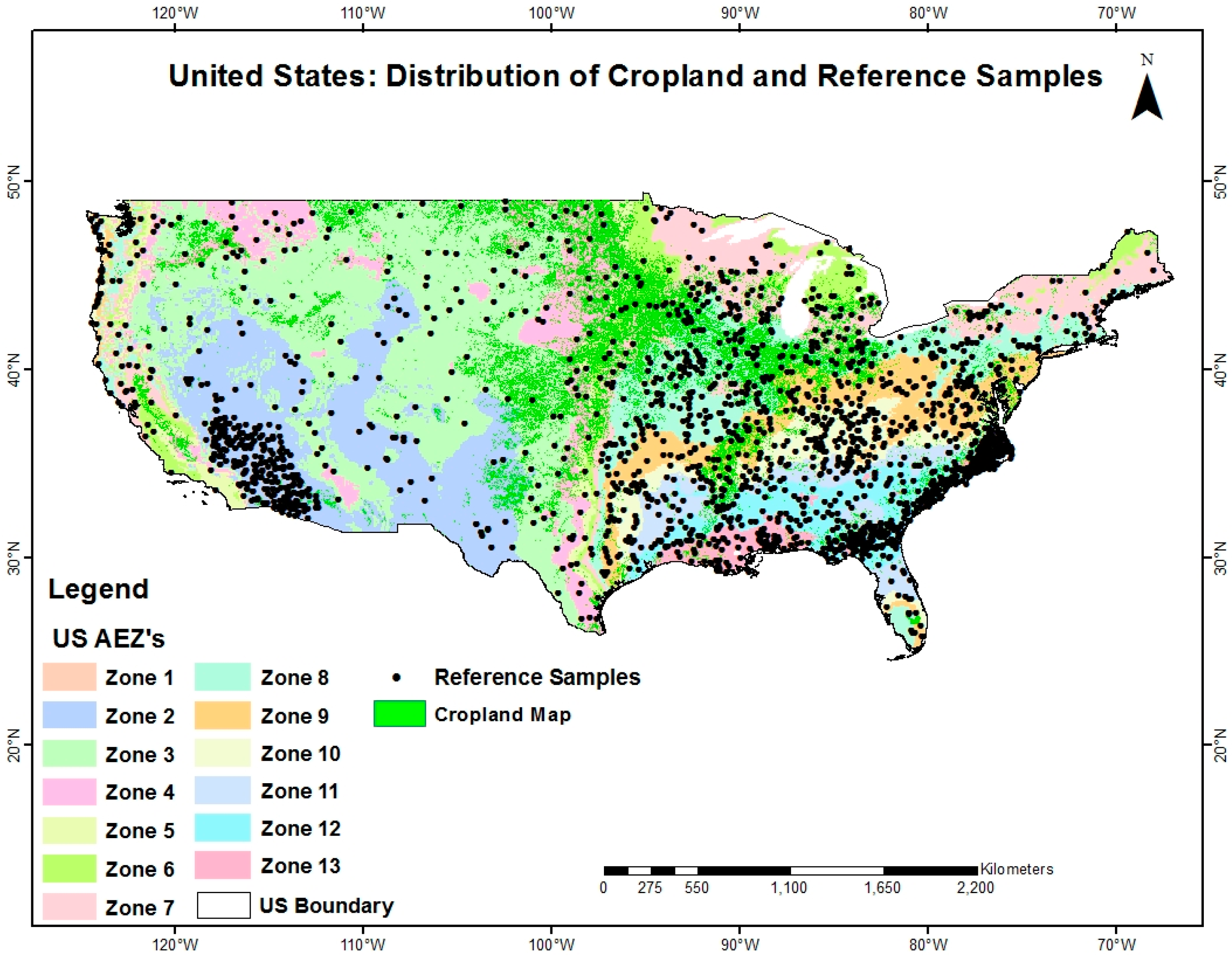
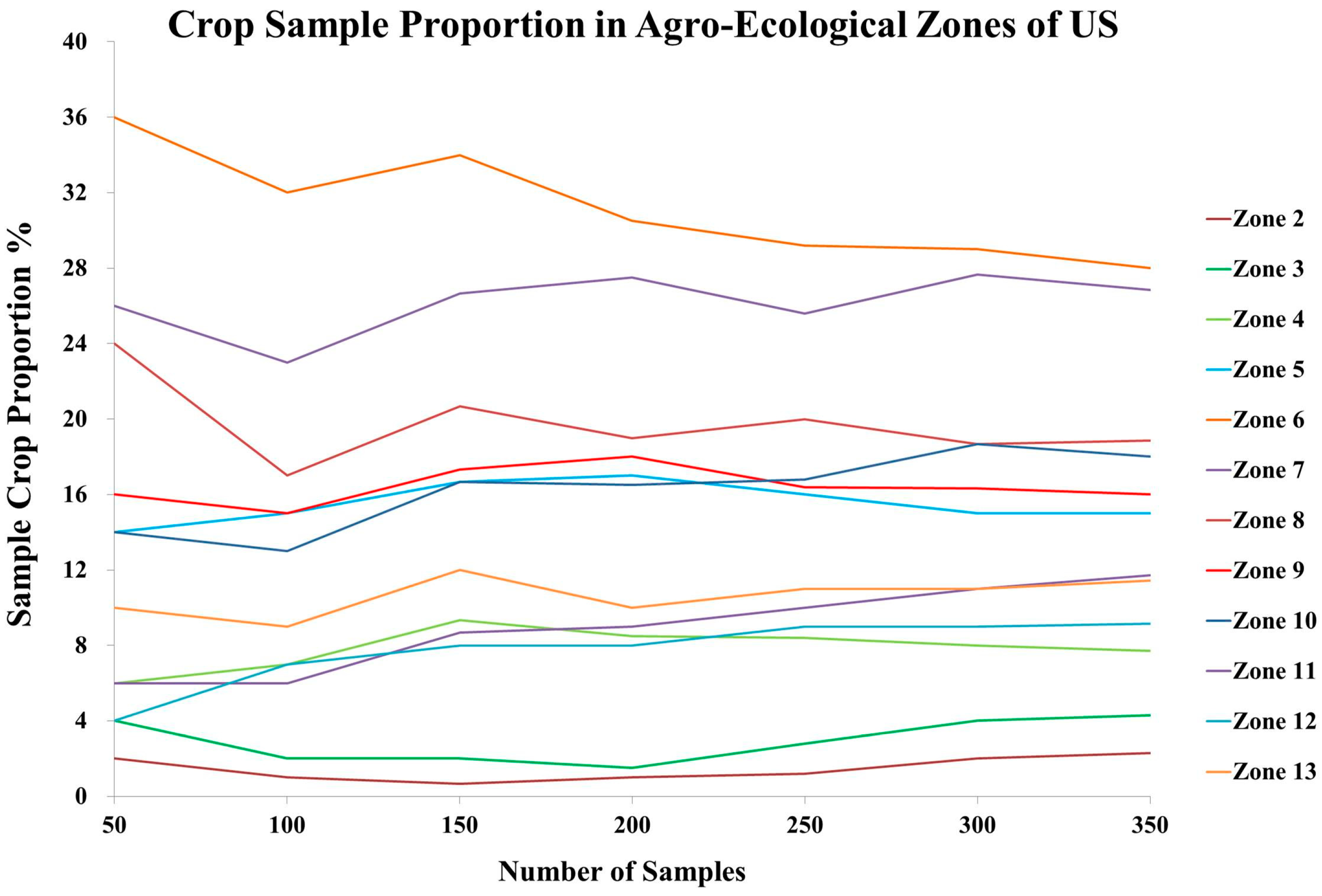
There is a great advantage in the US of having an extensive and easily accessible reference data set (i.e., USDA CDL). Due to the availability of such a high-quality reference data (i.e., accuracy ranges from 85–95%) [36], it was easy to perform an accuracy assessment of cropland maps in the US as compared to other continents. AEZ-based assessment strategy was employed with only a few modifications in the sampling design to choose an appropriate sample scheme and size. The task of achieving an appropriate sample size was determined by a sample simulation analysis that provided insight into how many samples were required to perform a continent specific accuracy assessment. Therefore, AEZ-based assessment strategy using high-quality reference data with some modifications in the sampling design was employed to report the accuracy measures in all the AEZ’s.

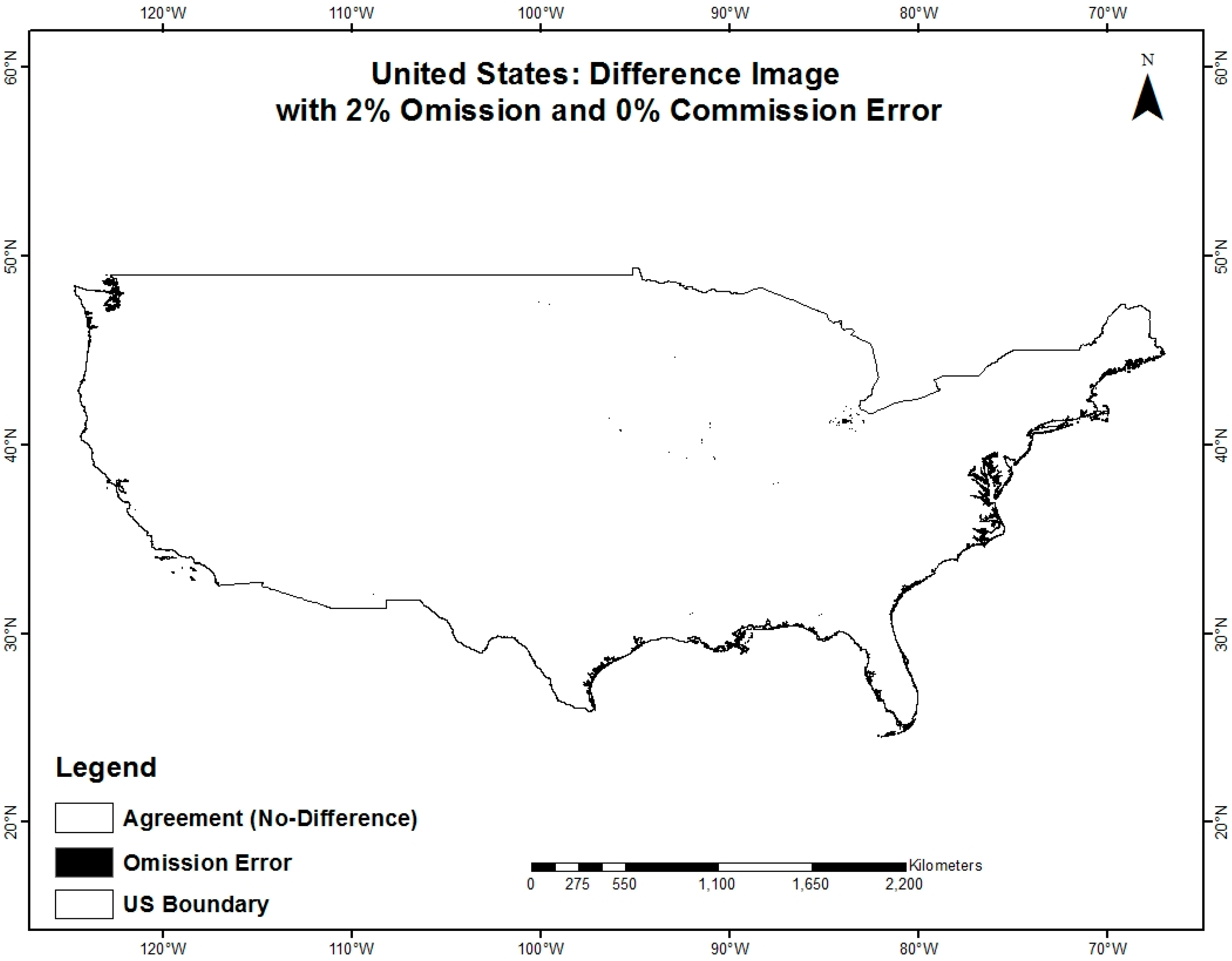
The accuracy assessment of cropland extent map in the US provided both accuracy measures in the form of error matrices and spatial distribution of agreement and disagreement in the form of a difference image. The compiled accuracy estimates generated for all the AEZ’s showed high overall accuracies for the crop and no-crop classes with no commission errors in the cropland areas (Table 1). These results were also confirmed with a difference image that showed spatial agreement and disagreement between the reference data and the map (Figure 6). The cropland class on the map has no-commission error and only 2% omission error. Overall, there were no complications in performing the accuracy assessment of the cropland maps of the US. The results show that performing an accuracy assessment of the cropland extent map for a continent with an extensive reference data set can easily be done, but that care still must be taken to determine homogeneous cropping regions which result in more meaningful, representative and valid mapping products.

4.2. Africa

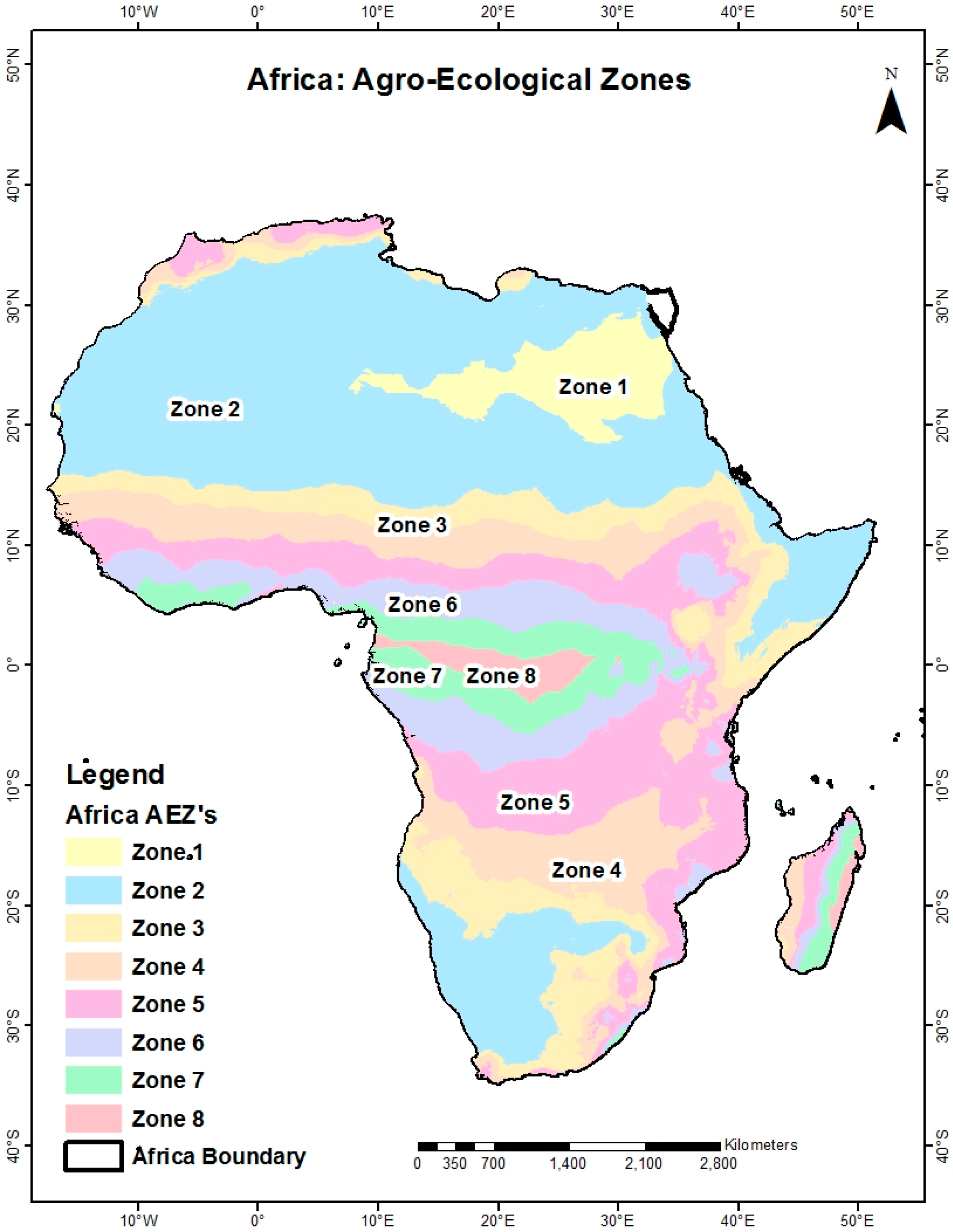
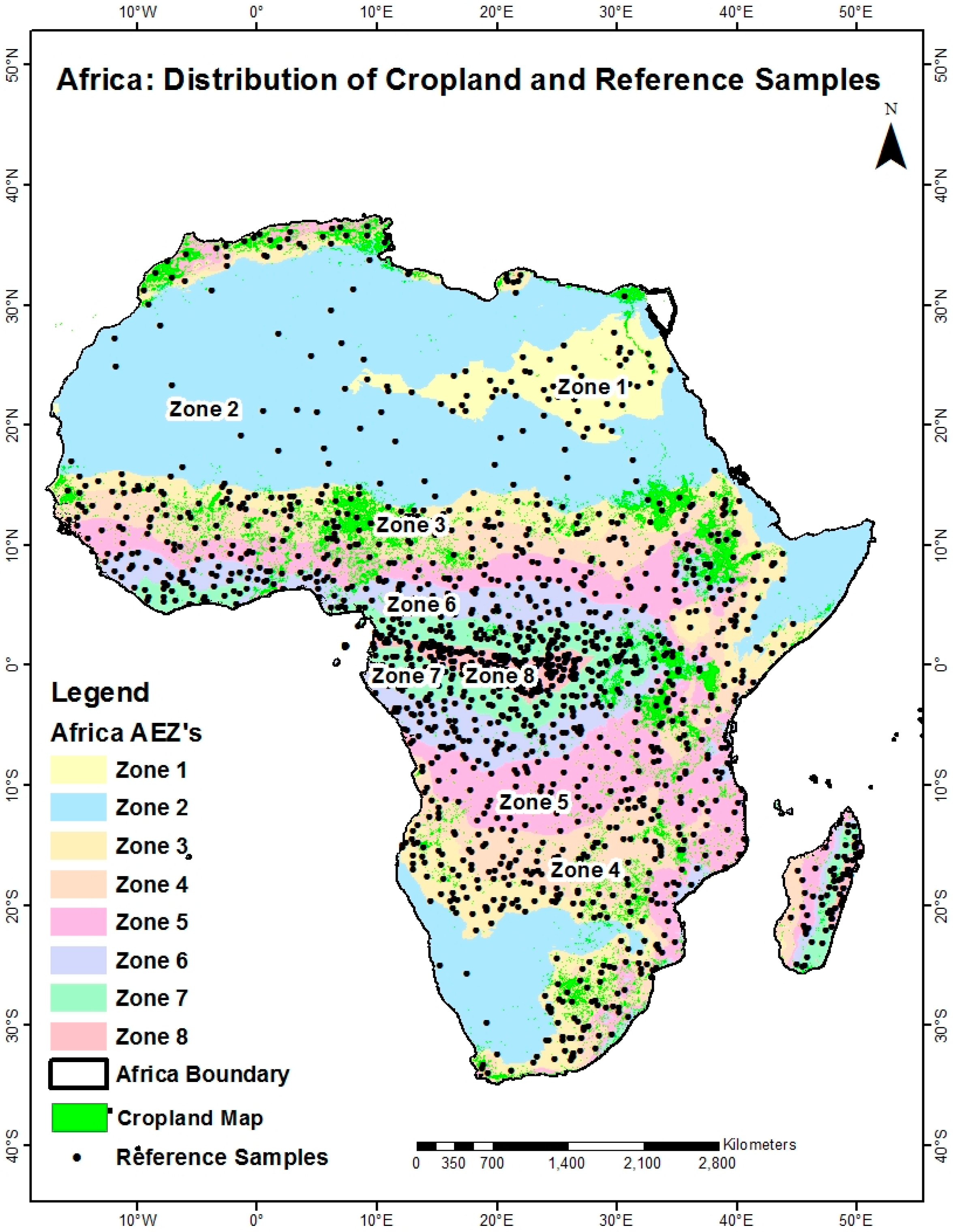
In Africa, different issues and constraints were observed when compared to the other selected continents due to: (1) the heterogeneous and scattered cropland distribution across the AEZ’s; and (2) the lack of effective and valid reference data. In Africa, AEZ’s were quite diverse from each other with a few zones having very sparse cropland distribution as compared to others where the cropland areas were more uniformly distributed. These issues and concerns were considered and planned for well before assessing the cropland maps using the AEZ-based accuracy assessment strategy with a modified sampling design. The AEZ-based strategy was different from the one employed in the US as it was specific to each AEZ according to each zone’s cropping pattern variability. In response to these cropping patterns and the lack of availability of valid reference data, the traditional method of accuracy assessment was conducted using a modified sampling design.

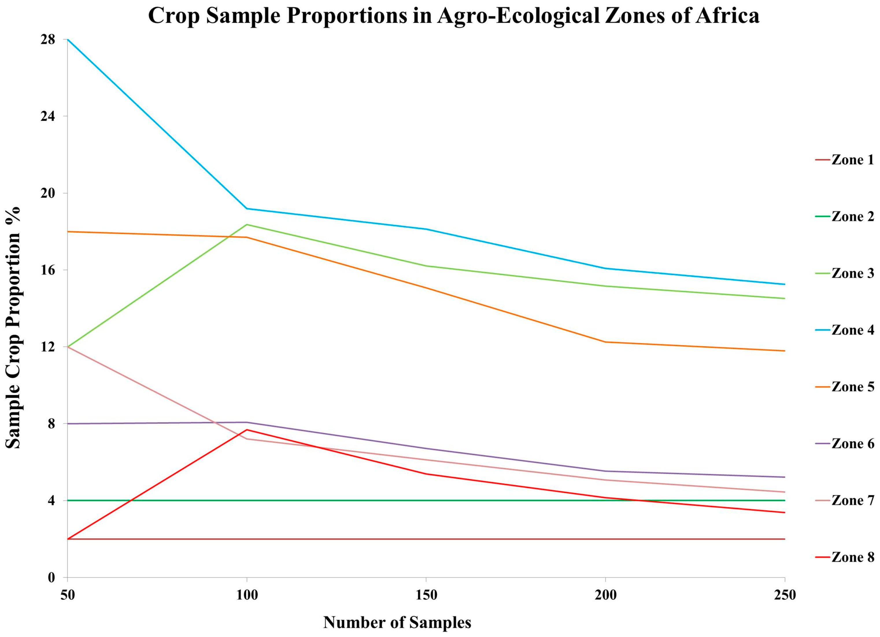
To perform the accuracy assessment of the cropland extent map of Africa, the reference data had to be collected from interpretation of VHRI for the year 2014 because no other data existed. Before collecting this reference data, it was necessary to determine where and how many samples were required. Another sampling simulation was performed to determine appropriate sample sizes for the various AEZs. Because of the large variability in the cropland distribution of the AEZ’s in Africa, zones with low crop diversity (i.e., AEZ 1 and 2) were sampled with a minimum number of samples (50) as compared to the other zones (250). Such modified sampling in Africa demonstrates the power of being able to selectively devote effort and time in collecting reference data based on the variability in the cropland distribution.

The results in Table 3 show that there is a high overall accuracy in all the zones. It is very important to note the producer’s and user’s accuracy of the crop class in each AEZ. In Zone 5, 6 and 7, the producer’s and user’s accuracy of the crop class are low due to low crop intensity and spatial structure of cropland areas. However, Zone 1 and 2 also has low crop proportion but the spatial structure of crop patches is different in these zones as compared to zone 5, 6 and 7. Therefore, different users’ and producers’ accuracies were observed in each zone due to spatial fragmentation of cropland areas in specific zones. These accuracies provide a more detailed view for each mapped class beyond just the overall accuracy and are indicative of the AEZ-based assessment strategy. Specific to Africa, it is very important to observe the cropping pattern in each AEZ and how much effort is required to generate the reference data necessary to perform the AEZ-based assessment strategy. These results show that the AEZ’s with low crop proportions do not require large sampling efforts as these zones have smaller geographic extent and less cropland area to assess. It is, therefore, reasonable to assume that if the sample size was increased for these zones; neither the number of crop samples nor the map accuracy would increase. Throughout this process of assessing the cropland map of Africa, the AEZ-based assessment strategy helped to provide a more detailed view of the accuracies of homogeneous regions within the continent.

4.3. Australia

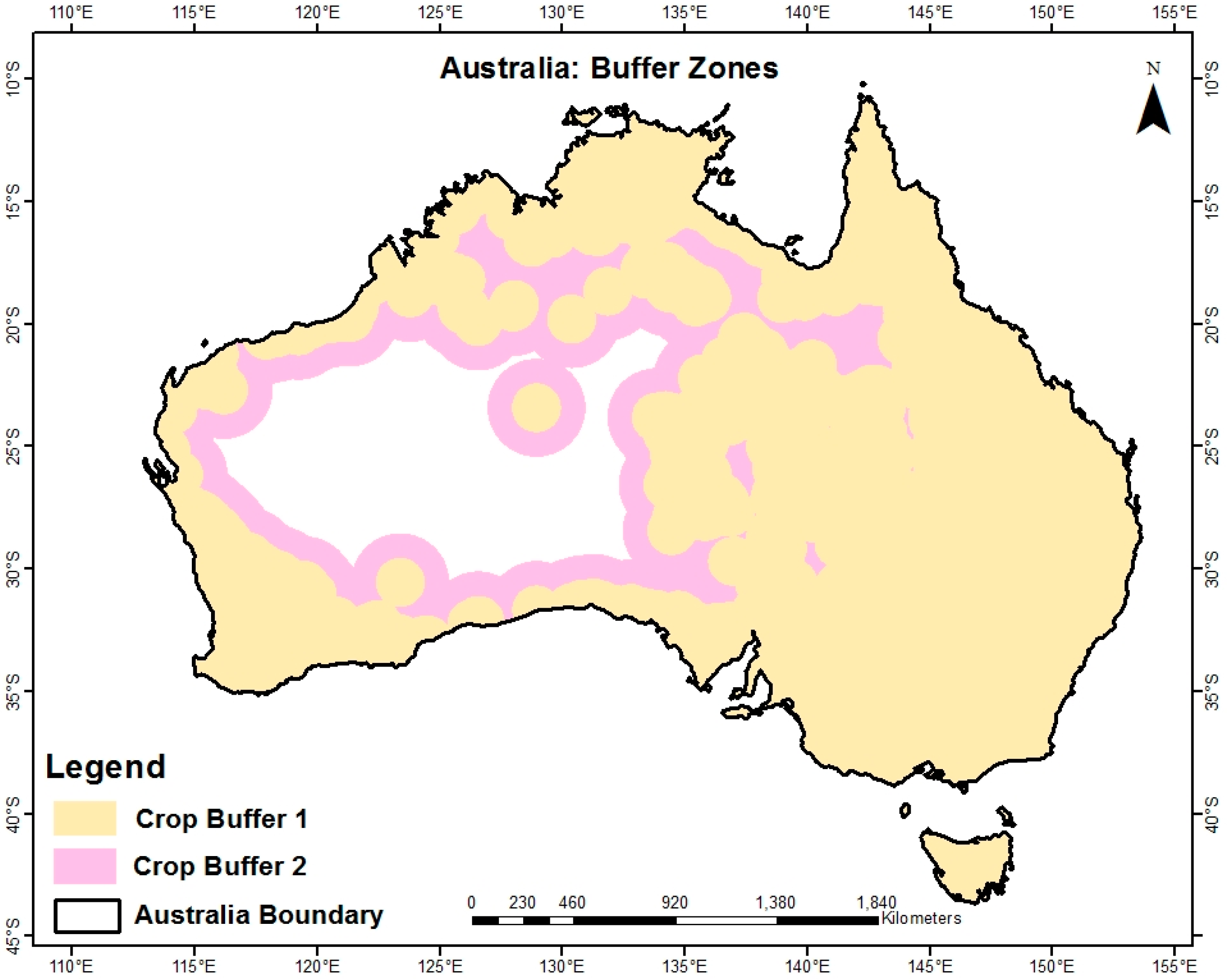
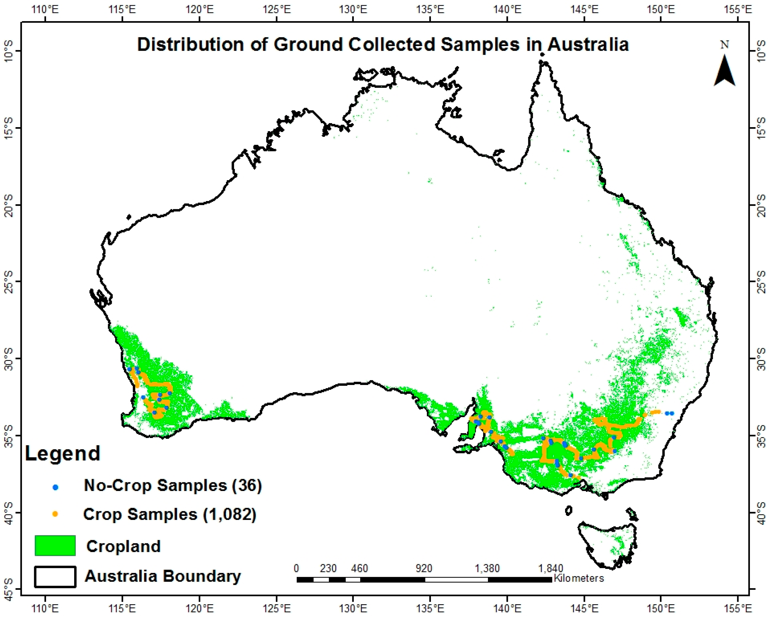
The accuracy assessment process to validate the cropland extent map of Australia was modified differently than the process used in the US and Africa. In Australia, the cropland distribution is concentrated only along a narrow belt towards the edges of the continent. There is a very low chance of cropland areas towards the center region of Australia because of the very dry conditions there. This concentrated cropping pattern was considered in the assessment strategy by choosing a reduced region around these cropland patches. AEZ’s in Australia do not exhibit much diversity due to low crop variability in the continent and therefore, were not appropriate to stratify the continent. Rather than an AEZ-based assessment strategy, a buffering approach was used to divide the continent into homogeneous regions to perform a valid assessment of the cropland map of Australia.

In addition to a different method of stratification, two different sources of reference data were used in Australia. The first were ground collected samples and the second were collected from interpretation of VHRI. As a result of the ground-collected reference data, a new set of issues needed to be considered. This ground data was collected during a field campaign that emphasized identifying cropland areas. As a result, very little non-cropland samples were recorded. 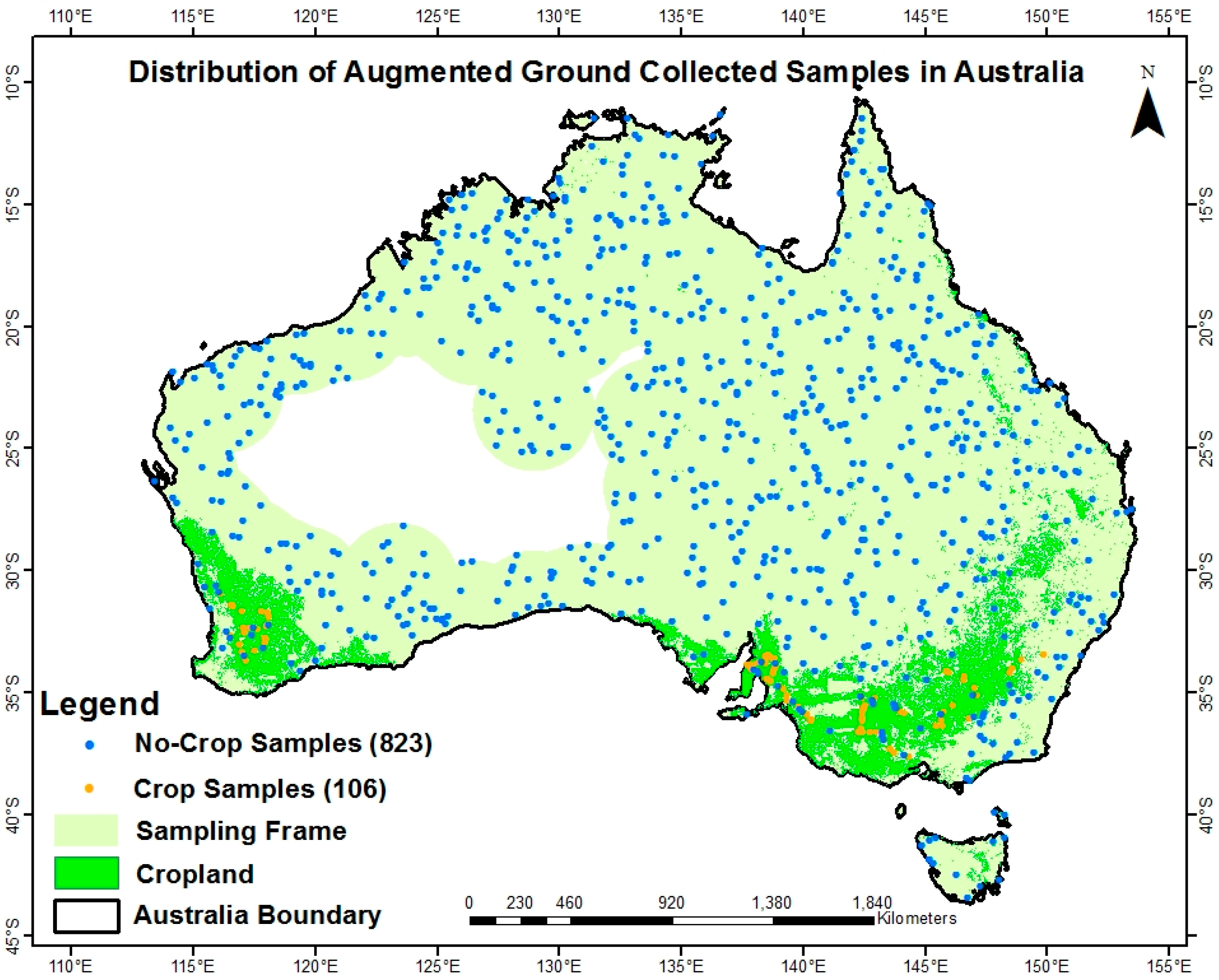Therefore, creating an error matrix from the reference data resulted in an error matrix in which there were many cropland samples and few non-cropland samples (Table 5). However, given that only approximately 12% of Australia is cropland, this error matrix was highly imbalanced and not representative of the map accuracy. The non-cropland samples were augmented appropriately using interpretation of VHRI to obtain sufficient samples to generate a balanced error matrix indicative of the actual cropland/non-cropland proportion (Table 6).

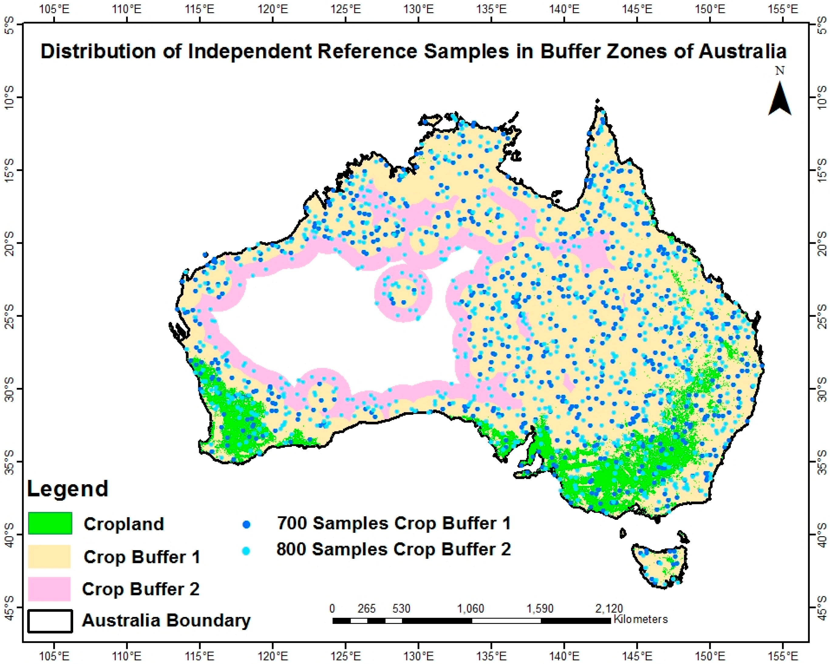
While the balanced error matrix generated from the ground reference data augmented with interpretation of VHRI demonstrates good overall cropland mapping, it is not representative of the entire continent since the ground data were collected all in the southern region. To solve this problem, a stratification approach using buffer analysis was adopted. This method provides a buffer around the cropland areas of Australia at two distances and eliminates sample collection from the center of the continent where there was very low chance of finding crops.

The error matrices generated for the buffer zones (Table 7 and Table 8) have high accuracies, but are lower than the error matrix in Table 6. However, these error matrices from the buffering approach should be viewed as more representative and meaningful than the matrix that used reference data from only part of the continent. As demonstrated in Australia, the entire continent might not be considered as an appropriate sampling area for assessing the accuracy of the cropland maps. In such places, therefore, the sampling area needs to be modified to accommodate sparse and concentrated cropping pattern to provide meaningful and representative accuracy results.

5. Lessons Learned

Accuracy assessment is an expensive, yet essential, component of the mapping projects. Maps without their associated accuracy estimates will not be valuable to the users [28,46]. While there is a well-established traditional method to perform the accuracy assessment of thematic maps [30], there remains considerable need for future research and development to perform the accuracy assessment of large area thematic maps. There are few important lessons that were learned from a modified assessment strategy conducted for three different continents while assessing large area cropland extent maps:

• Before assessing the cropland extent maps of different continents, some sort of stratification must be employed to divide the area into homogeneous regions. The stratification approach must be considered and recommended to address the issues of variation in different agricultural landscapes within each continent.
• It is important to ensure that the accuracy assessment of large area cropland extent maps is performed in accordance with how the map was created. Failure to consider the methodologies used including any stratification that was performed will result in unresolved issues.
• In order to conduct a modified accuracy assessment for the homogeneous regions within the continent, different issues, constraints and characteristics observed in the cropland maps for different continents must be considered carefully. These issues can be either related to complex agricultural landscapes or the availability of reference data for different continents.
• Performing an accuracy assessment for a continent with an extensive reference data can be easily done, but still the sampling scheme and size must be modified carefully to determine enough samples for the homogeneous cropping regions to result in meaningful, representative and valid mapping products.
• A modified sampling scheme and size must be chosen using a sample analysis approach for each homogeneous region in response to their cropping pattern variability. Such modified sampling can demonstrate the power of being able to selectively devote effort and time in collecting reference data based on the cropping pattern variability.
• Any ground collected samples especially if only certain map classes (i.e., crops) area collected must be augmented to create a balanced and effective reference data set. However, this balanced error still might be representative of the entire continent if the ground data were collected in only one region.
• When the entire continent cannot be considered as an appropriate sampling area for assessing the accuracy of cropland maps, the sampling area should be modified to accommodate the sparse and concentrated cropping pattern using stratification method.

6. Conclusions

This paper presents modified accuracy assessment strategies used to assess the accuracy of large area cropland extent maps in response to different issues such as variations of cropping pattern and reference data availability in different continents. Considering and addressing these issues, the modified assessment strategies helped to understand the efficacy and quality of cropland extent maps for different agricultural landscapes to implement economic planning and policymaking. The information derived from large area cropland maps with agricultural landscapes of different continents can be enriched, improved and analyzed with modified assessment strategies. Such modified assessment strategies promise to achieve more meaningful, representative and applicable mapping products for each continent. Therefore, the need for a continent-specific assessment strategy developed by modifying the sampling design for collecting reference data and computing accuracy measures was demonstrated to be valuable. However, different sampling methods can be employed and compared in the future to analyze the accuracy results for different cropping scenarios.

A modified assessment strategy was employed to assess the accuracy of the cropland extent maps of three selected continents developed as a part of GFSAD project. The variability of cropping pattern in the agricultural landscapes and reference data availability were considered and addressed to provide meaningful and valid accuracy results for mapping products within these selected continents. The stratification approach based on AEZ’s or buffer zones used to divide the continent into homogeneous cropping regions: (1) minimized the heterogeneity of different cropping patterns and (2) helped to rationalize the validation efforts for different continents. Finally, the sampling scheme and size were modified for the homogeneous regions using a sample analysis approach based on the variations of cropping pattern within the continent.

In summary, continent-specific modified assessments performed for three selected continents demonstrate that the accuracy assessment can be easily done for a continent such as the US with extensive availability of a reference dataset while more modifications were needed in the sampling scheme for the continents with little to no reference datasets. The result of the modified sampling performed in the AEZ’s of Africa show that the effort and time in collecting reference data can be selectively devoted based on the variability in the cropland distribution. Finally, a modified sampling was employed in the buffer zones of Australia using two different sources of reference data. An unbalanced number of ground samples collected during a field campaign that emphasized identifying cropland areas were augmented and balanced to be indicative of the crop/no crop area proportion of the map to generate a balanced and valid error matrix for Australia. The analysis performed with this modified strategy shows that the entire continent might not be considered as an appropriate sampling area for assessing the cropland maps due to little chance of cropland in center of Australia because of extremely dry conditions.

References

1. Wu, Z.; Thenkabail, P.S.; Mueller, R.; Zakzeski, A.; Melton, F.; Johnson, L.; Rosevelt, C.; Dwyer, J.; Jones, J.; Verdin, J.P. Seasonal cultivated and fallow cropland mapping using MODIS-based automated cropland classification algorithm. J. Appl. Remote Sens. 2014, 8, 83618–83685. [Google Scholar] [CrossRef]
2. Giri, C.; Pengra, B.; Long, J.; Loveland, T.R. Next generation of global land cover characterization, mapping, and monitoring. Int. J. Appl. Earth Obs. Geoinf. 2013, 25, 30–37. [Google Scholar] [CrossRef]
3. Olofsson, P.; Stehman, S.V.; Woodcock, C.E.; Sulla-Menashe, D.; Sibley, A.M.; Newell, J.D.; Friedl, M.A.; Herold, M. A global land-cover validation data set, part I: Fundamental design principles. Int. J. Remote Sens. 2012, 33, 5768–5788. [Google Scholar] [CrossRef]
4. Pflugmacher, D.; Krankina, O.N.; Cohen, W.B.; Friedl, M.A.; Sulla-Menashe, D.; Kennedy, R.E.; Nelson, P.; Loboda, T.V.; Kuemmerle, T.; Dyukarev, E.; et al. Comparison and assessment of coarse resolution land cover maps for Northern Eurasia. Remote Sens. Environ. 2011, 115, 3539–3553. [Google Scholar] [CrossRef]
5. Fritz, S.; See, L. Identifying and quantifying uncertainty and spatial disagreement in the comparison of Global Land Cover for different applications. Glob. Chang. Biol. 2008, 14, 1057–1075. [Google Scholar] [CrossRef]
6. Husak, G.J.; Marshall, M.T.; Michaelsen, J.; Pedreros, D.; Funk, C.; Galu, G. Crop area estimation using high and medium resolution satellite imagery in areas with complex topography. J. Geophys. Res. Atmos. 2008, 113. [Google Scholar] [CrossRef]
7. Thenkabail, P.S.; Wu, Z. An automated cropland classification algorithm (ACCA) for Tajikistan by combining landsat, MODIS, and secondary data. Remote Sens. 2012, 4, 2890–2918. [Google Scholar] [CrossRef]
8. Grekousis, G.; Mountrakis, G.; Kavouras, M. An overview of 21 global and 43 regional land-cover mapping products. Int. J. Remote Sens. 2015, 36, 5309–5335. [Google Scholar] [CrossRef]
9. Foody, G.M. Valuing map validation: The need for rigorous land cover map accuracy assessment in economic valuations of ecosystem services. Ecol. Econ. 2015, 111, 23–28. [Google Scholar] [CrossRef]
10. Fritz, S.; See, L.; You, L.; Justice, C.; Becker-Reshef, I.; Bydekerke, L.; Cumani, R.; Defourny, P.; Erb, K.; Foley, J.; et al. The need for improved maps of global cropland. Eos Trans. Am. Geophys. Union 2013, 94, 31–32. [Google Scholar] [CrossRef]
11. Gallego, F.J.; Kussul, N.; Skakun, S.; Kravchenko, O.; Shelestov, A.; Kussul, O. Efficiency assessment of using satellite data for crop area estimation in Ukraine. Int. J. Appl. Earth Obs. Geoinf. 2014, 29, 22–30. [Google Scholar] [CrossRef]
12. Wu, W.; Shibasaki, R.; Yang, P.; Zhou, Q.; Tang, H. Remotely sensed estimation of cropland in China: A comparison of the maps derived from four global land cover datasets. Can. J. Remote Sens. 2008, 34, 467–479. [Google Scholar] [CrossRef]
13. Barrett, E.C. Introduction to Environmental Remote Sensing, 1st ed.; Routledge: Abingdon, UK, 2013. [Google Scholar]
14. Thenkabail, P.S.; Lyon, G.J.; Turral, H.; Biradar, C. Remote Sensing of Global Croplands for Food Security; CRC Press-Taylor and Francis Group: Boca Raton, FL, USA; London, UK, 2009; p. 556. [Google Scholar]
15. Portmann, F.T.; Siebert, S.; Döll, P. MIRCA2000—Global monthly irrigated and rainfed crop areas around the year 2000: A new high-resolution data set for agricultural and hydrological modeling. Glob. Biogeochem. Cycles 2010, 24, 1–24. [Google Scholar] [CrossRef]
16. Salmon, J.M.; Friedl, M.A.; Frolking, S.; Wisser, D.; Douglas, E.M. Global rain-fed, irrigated, and paddy croplands: A new high resolution map derived from remote sensing, crop inventories and climate data. Int. J. Appl. Earth Obs. Geoinf. 2015, 38, 321–334. [Google Scholar] [CrossRef]
17. Pittman, K.; Hansen, M.C.; Becker-Reshef, I.; Potapov, P.V.; Justice, C.O. Estimating global cropland extent with multi-year MODIS data. Remote Sens. 2010, 2, 1844–1863. [Google Scholar] [CrossRef]
18. Massey, R.; Sankey, T.T.; Congalton, R.G.; Yadav, K.; Thenkabail, P.S.; Ozdogan, M.; Sánchez Meador, A.J. MODIS phenology-derived, multi-year distribution of conterminous U.S. crop types. Remote Sens. Environ. 2017, 198, 490–503. [Google Scholar] [CrossRef]
19. Xiong, J.; Thenkabail, P.S.; Gumma, M.K.; Teluguntla, P.; Poehnelt, J.; Congalton, R.G.; Yadav, K.; Thau, D. Automated cropland mapping of continental Africa using Google Earth Engine cloud computing. ISPRS J. Photogramm. Remote Sens. 2017, 126, 225–244. [Google Scholar] [CrossRef]
20. Teluguntla, P.; Thenkabail, P.S.; Xiong, J.; Gumma, M.K.; Congalton, R.G.; Oliphant, A.; Poehnelt, J.; Yadav, K.; Rao, M.; Massey, R. Spectral matching techniques (SMTs) and automated cropland classification algorithms (ACCAs) for mapping croplands of Australia using MODIS 250-m time-series (2000–2015) data. Int. J. Digit. Earth 2017, 10, 944–977. [Google Scholar] [CrossRef]
21. Global Croplands. Available online: https://www.croplands.org/app/map?lat=0&lng=0&zoom=2 (accessed on 5 March 2017).
22. Tsendbazar, N.E.; de Bruin, S.; Herold, M. Assessing global land cover reference datasets for different user communities. ISPRS J. Photogramm. Remote Sens. 2015, 103, 93–114. [Google Scholar] [CrossRef]
23. Foody, G.M. Status of land cover classification accuracy assessment. Remote Sens. Environ. 2002, 80, 185–201. [Google Scholar] [CrossRef]
24. Congalton, R.G.; Green, K. Assessing the Accuracy of Remotely Sensed Data-Principles and Practices, 2nd ed.; CRC Press: Boca Raton, FL, USA, 2009; ISBN 9781420055122. [Google Scholar]
25. DeGloria, S.D.; Laba, M.; Gregory, S.K.; Braden, J.; Ogurcak, D.; Hill, E.; Fegraus, E.; Fiore, J.; Stalter, A.; Beecher, J.; et al. Conventional and fuzzy accuracy assessment of land cover maps at regional scale. In Proceedings of the 4th International Symposium on Spatial Accuracy Assessment in Natural Resources and Environmental Sciences, Amsterdam, The Netherlands, 11–13 July 2000. [Google Scholar]
26. Ung, C.H.; Lambert, M.C.; Guidon, L.; Fournier, R.A. Integrating Landsat-TM data with environmental data for classifying forest cover types and estimating their biomass. In Proceedings of the 4th International Symposium on Spatial Accuracy Assessment in Natural Resources and Environmental Sciences, Amsterdam, The Netherlands, 12–14 July 2000; pp. 659–662. [Google Scholar]
27. Fritz, S.; See, L.; Mccallum, I.; You, L.; Bun, A.; Moltchanova, E.; Duerauer, M.; Albrecht, F.; Schill, C.; Perger, C.; et al. Mapping global cropland and field size. Glob. Chang. Biol. 2015, 21, 1980–1992. [Google Scholar] [CrossRef] [PubMed] [Green Version]
28. Strahler, A.H.; Boschetti, L.; Foody, G.M.; Friedl, M.A.; Hansen, M.C.; Herold, M.; Mayaux, P.; Morisette, J.T.; Stehman, S.V.; Woodcock, C.E. Global Land Cover Validation: Recommendations for Evaluation and Accuracy Assessment of Global Land Cover Maps. GOFC-GOLD Report No. 25. European Commission Joint Research Centre, 2006; pp. 48–51. Available online: http://nofc.cfs.nrcan.gc.ca/gofc-gold/Report%20Series/GOLD_25.pdf (accessed on 10 April 2017).
29. Foody, G.M. Local characterization of thematic classification accuracy through spatially constrained confusion matrices. Int. J. Remote Sens. 2005, 37–41. [Google Scholar] [CrossRef]
30. Congalton, R.G.; Green, K. Assessing the Accuracy of Remotely Sensed Data: Principles and Practices, 1st ed.; CRC Press: Boca Raton, FL, USA, 1999; ISBN 1420055127. [Google Scholar]
31. Congalton, R.G. A review of assessing the accuracy of classifications of remotely sensed data. Remote Sens. Environ. 1991, 37, 35–46. [Google Scholar] [CrossRef]
32. Wardlow, B.D.; Egbert, S.L. Large-area crop mapping using time-series MODIS 250 m NDVI data: An assessment for the U.S. Central Great Plains. Remote Sens. Environ. 2008, 112, 1096–1116. [Google Scholar] [CrossRef]
33. Stehman, S.V. Selecting and interpreting measures of thematic classification accuracy. Remote Sens. Environ. 1997, 62, 77–89. [Google Scholar] [CrossRef]
34. Ramankutty, N.; Evan, A.T.; Monfreda, C.; Foley, J.A. Farming the planet: 1. Geographic distribution of global agricultural lands in the year 2000. Glob. Biogeochem. Cycles 2008, 22, 1–19. [Google Scholar] [CrossRef]
35. Fischer, G.; Nachtergaele, F.O.; Prieler, S.; Teixeira, E.; Toth, G.; van Velthuizen, H.; Verelst, L.; Wiberg, D. Global Agro-Ecological Zones (GAEZ): Model Documentation; International Institute of Applied Systems Analysis: Laxenburg, Austria; Food and Agricultural Organization: Rome, Italy, 2012; pp. 1–179. [Google Scholar]
36. Boryan, C.; Yang, Z.; Mueller, R.; Craig, M. Monitoring US agriculture: The US department of agriculture, national agricultural statistics service, Cropland data layer program. Geocarto Int. 2011, 26, 341–358. [Google Scholar] [CrossRef]
37. Leff, B.; Ramankutty, N.; Foley, J.A. Geographic distribution of major crops across the world. Glob. Biogeochem. Cycles 2004, 18. [Google Scholar] [CrossRef]
38. Shao, Y.; Lunetta, R.S. Comparison of support vector machine, neural network, and CART algorithms for the land-cover classification using limited training data points. ISPRS J. Photogramm. Remote Sens. 2012, 70, 78–87. [Google Scholar] [CrossRef]
39. Champagne, C.; McNairn, H.; Daneshfar, B.; Shang, J. A bootstrap method for assessing classification accuracy and confidence for agricultural land use mapping in Canada. Int. J. Appl. Earth Obs. Geoinf. 2014, 29, 44–52. [Google Scholar] [CrossRef]
40. Vancutsem, C.; Marinho, E.; Kayitakire, F.; See, L.; Fritz, S. Harmonizing and combining existing land cover/land use datasets for cropland area monitoring at the African continental scale. Remote Sens. 2013, 5, 19–41. [Google Scholar] [CrossRef] [Green Version]
41. Waldner, F.; Canto, G.S.; Defourny, P. Automated annual cropland mapping using knowledge-based temporal features. ISPRS J. Photogramm. Remote Sens. 2015, 110, 1–13. [Google Scholar] [CrossRef]
42. Van Wart, J.; van Bussel, L.G.J.; Wolf, J.; Licker, R.; Grassini, P.; Nelson, A.; Boogaard, H.; Gerber, J.; Mueller, N.D.; Claessens, L.; et al. Use of agro-climatic zones to upscale simulated crop yield potential. Field Crop. Res. 2013, 143, 44–55. [Google Scholar] [CrossRef] [Green Version]
43. Di Vittorio, A.V.; Kyle, P.; Collins, W.D. What are the effects of Agro-Ecological Zones and land use region boundaries on land resource projection using the Global Change Assessment Model? Environ. Model. Softw. 2016, 85, 246–265. [Google Scholar] [CrossRef]
44. Seo, S.N. Evaluation of the Agro-Ecological Zone methods for the study of climate change with micro farming decisions in sub-Saharan Africa. Eur. J. Agron. 2014, 52, 157–165. [Google Scholar] [CrossRef]
45. Stehman, S.V.; Czaplewski, R.L. Design and analysis for thematic map accuracy assessment—An application of satellite imagery. Remote Sens. Environ. 1998, 64, 331–344. [Google Scholar] [CrossRef]
46. Thenkabail, P.S. Assessing positional and thematic accuracies of map generated from remotely sensed data. In Remotely Sensed Data Characterization, Classification, and Accuracies; CRC Press-Taylor and Francis Group: Boca Raton, FL, USA, 2005; pp. 583–605. [Google Scholar]
47. Congalton, R.G.; Gu, J.; Yadav, K.; Thenkabail, P.; Ozdogan, M. Global land cover mapping: A review and uncertainty analysis. Remote Sens. 2014, 6, 12070–12093. [Google Scholar] [CrossRef]
48. Ginevan, M.E. Testing land-use map accuracy: Another look. Photogramm. Eng. Remote Sens. 1979, 45, 1371–1377. [Google Scholar]
49. Hord, R.M.; Brooner, W. Land-use map accuracy criteria. Photogramm. Eng. Remote Sens. 1976, 42, 671–677. [Google Scholar]
50. Stehman, S.V. Comparison of systematic and random sampling for estimating the accuracy of maps generated from remotely sensed data. Photogramm. Eng. Remote Sens. 1992, 58, 1343–1350. [Google Scholar]
51. Stehman, S.V. Sampling designs for accuracy assessment of land cover. Int. J. Remote Sens. 2009, 30, 5243–5272. [Google Scholar] [CrossRef]
52. Van Genderen, J.; Lock, B. Testing land use map accuracy. Photogramm. Eng. Remote Sens. 1977, 43, 1135–1137. [Google Scholar]
53. Congalton, R.G. A comparison of sampling schemes used in generating error matrices for assessing the accuracy of maps generated from remotely sensed data. Photogramm. Eng. Remote Sens. 1988, 54, 593–600. [Google Scholar]
54. Hay, A.M. Sampling designs to test land use map accuracy. Photogramm. Eng. Remote Sens. 1979, 45, 529–533. [Google Scholar]
55. Rosenfield, G.H.; Fitzpatrick-Lins, K.; Ling, H.S. No Sampling for thematic map accuracy testing. Photogramm. Eng. Remote Sens. 1982, 48, 131–137. [Google Scholar]
56. Story, M.; Congalton, R.G. Accuracy assessment: A user’s perspective. Photogramm. Eng. Remote Sens. 1986, 52, 397–399. [Google Scholar] [CrossRef]
57. CropScape—Cropland Data Layer, United States Department of Agriculture, National Agricultural Statistics Service. Available online: https://nassgeodata.gmu.edu/CropScape (accessed on 7 March 2017).
Figure 1. Map showing the location of three selected continents and their respective homogeneous regions such as agro-ecological zones (AEZs) and crop buffer.
Remotesensing 10 00053 g001
Figure 2. Flowchart of the process used to conduct the continent-based accuracy assessment of the GFSAD mapping products.
Remotesensing 10 00053 g002
Figure 3. The distribution of Agro-ecological zones in the United States.
Remotesensing 10 00053 g003
Figure 4. The graphical representation of sample size simulation in AEZ’s of the US.
Remotesensing 10 00053 g004
Figure 5. The distribution of randomly generated reference samples within each of the AEZ’s of the US.
Remotesensing 10 00053 g005
Figure 6. The difference image derived using reference data and cropland map of the US showing 2% Omission and 0% commission error.
Remotesensing 10 00053 g006
Figure 7. Agro-Ecological Zones (AEZ’s) of Africa.
Remotesensing 10 00053 g007
Figure 8. The graph showing the sample simulation in AEZ’s of Africa.
Remotesensing 10 00053 g008
Figure 9. The distribution of Cropland and Reference Samples in Africa.
Remotesensing 10 00053 g009
Figure 10. Crop buffer zones delineated using Euclidean Distance buffering approach.
Remotesensing 10 00053 g010
Figure 11. The distribution of ground collected samples used in the accuracy assessment of cropland map of Australia.
Remotesensing 10 00053 g011
Figure 12. The distribution of ground collected and augmented no-crop samples in Australia.
Remotesensing 10 00053 g012
Figure 13. The distribution of reference samples in buffer zones of Australia.
Remotesensing 10 00053 g013