Downscaling GRACE Remote Sensing Datasets to High-Resolution Groundwater Storage Change Maps of California’s Central Valley

Abstract

NASA’s Gravity Recovery and Climate Experiment (GRACE) has already proven to be a powerful data source for regional groundwater assessments in many areas around the world. However, the applicability of GRACE data products to more localized studies and their utility to water management authorities have been constrained by their limited spatial resolution (~200,000 km²). Researchers have begun to address these shortcomings with data assimilation approaches that integrate GRACE-derived total water storage estimates into complex regional models, producing higher-resolution estimates of hydrologic variables (~2500 km²). Here we take those approaches one step further by developing an empirically based model capable of downscaling GRACE data to a high-resolution (~16 km²) dataset of groundwater storage changes over a portion of California’s Central Valley. The model utilizes an artificial neural network to generate a series of high-resolution maps of groundwater storage change from 2002 to 2010 using GRACE estimates of variations in total water storage and a series of widely available hydrologic variables (PRISM precipitation and temperature data, digital elevation model (DEM)-derived slope, and Natural Resources Conservation Service (NRCS) soil type). The neural network downscaling model is able to accurately reproduce local groundwater behavior, with acceptable Nash-Sutcliffe efficiency (NSE) values for calibration and validation (ranging from 0.2445 to 0.9577 and 0.0391 to 0.7511, respectively). Ultimately, the model generates maps of local groundwater storage change at a 100-fold higher resolution than GRACE gridded data products without the use of computationally intensive physical models. The model’s simulated maps have the potential for application to local groundwater management initiatives in the region.

1. Introduction

Groundwater monitoring has historically relied on a network of local observations of well levels, or in situ measurements. In the United States, the United States Geological Survey (USGS) maintains a network of 850,000 active monitoring wells that provides fundamental data on groundwater quantity and quality [1] and enables essential regional studies [2,3]. In many other parts of the world, however, groundwater observation networks often lack adequate spatial and temporal coverage, they are often underfunded, and therefore they may well be unreliable [4,5]. Even in the United States, where a relative abundance of well data provides information to water managers on short- and long-term water level trends at specific locations, more monitoring sites are needed to better understand the groundwater surface and the spatial distribution of pumping patterns [1].

To overcome the shortcomings from sparse observation networks and insufficient in situ data, significant progress has been made in the way the groundwater surface and its behavior are represented. These advances have come from the fields of groundwater modeling [2,6,7,8], monitoring network design [9], and geostatistical analysis of groundwater data [10,11,12]. While this research has made huge strides in characterizing groundwater from limited data, many of these studies focused on small, sub-basin scales and represented limitations to capture wider spatial trends in groundwater.

Satellite remote sensing can complement existing monitoring networks and modeling studies, and can help compensate for gaps in spatial and temporal coverage. In particular, several authors have now demonstrated that NASA’s Gravity Recovery and Climate Experiment (GRACE) can reliably measure monthly groundwater storage changes in the large aquifer systems of the world [13,14,15]. Some examples include the Ogallala aquifer [16], northwestern India [17], California’s Central Valley [18], South America’s Guarani aquifer [19], the Middle East [20], the North China Plain [21], and several others [22,23,24].

Despite these studies, the ability of GRACE to monitor changes at finer scales, which could directly benefit local water management authorities, is limited. This is largely due to the low spatial resolution of its observations (~200,000 km²), and researchers and hydrogeologists have noted these drawbacks [25,26]. The lack of ground truthing and the potential errors in retrieval algorithms are also cited as deficiencies in remotely sensed data [27]. A higher-resolution GRACE data product would significantly improve information availability for local-scale decision makers, as well as offer novel data for regions that do not have adequate in situ monitoring networks.

To complement the shortage in regional in situ data and improve upon the resolution of GRACE data, this study downscales GRACE and creates a hybrid product that utilizes available local observations along with GRACE estimates of changes in total water storage to accurately characterize local changes in groundwater availability. Our approach has potential for use in data-scarce regions world-wide, as it requires only minimal hydrologic data and GRACE estimates of changes in total water storage to simulate groundwater storage change in a complex aquifer system.

1.1. Downscaling GRACE Data

The majority of research approaches for downscaling remote satellite data originate in the climate modeling literature, owing to the need to better understand the regional impacts of global change. Two approaches, dynamical and statistical, are the most common [28]. Dynamical methods typically utilize a higher-resolution, physically-based model using low-resolution data, such as those from a global climate model or general circulation model, as the lateral boundary conditions. Previous data assimilation approaches with GRACE have effectively been a form of dynamical downscaling [29]. Monthly GRACE observations of terrestrial water storage change (i.e., the change in the sum of snow, surface water, soil moisture, and groundwater) were assimilated into a physically based land surface model at the scale of the major watersheds of the Mississippi River Basin [29]. The output of the physical models—the higher-resolution, modeled water storage changes within the major watersheds—was forced to sum to the lower-resolution assimilated constraint from GRACE. The physics of the land surface modeling and atmospheric forcings were used to distribute the GRACE data to finer scales. Schumacher et al. (2017) combine GRACE data on total water storage (TWS) with a conceptual ~500 km resolution model to improve drought simulations within the Murray–Darling Basin, Australia [30]. Their results show that a simultaneous calibration and data assimilation approach that incorporates GRACE data leads to more accurate groundwater model simulations. Data assimilation methods have the strong advantage of being physically consistent but, at the same time, require significant computational time, limiting their applicability [31].

Statistical downscaling methods, instead, draw upon relationships between coarser-scale input data and finer-resolution target data [32]. A variety of statistical techniques have been applied and studied in the downscaling literature, including classification-based methods, regression models, Markov chains, statistical inversion [33], and stochastic models [34]. The advantages of these methods are that they are relatively flexible to various data types and spatial and temporal scales, they can generate uncertainty estimates of parameters and model output, and they are generally easy to apply [34]. Statistical methods are, however, based on the assumptions that the input and target data fully capture the dynamics of the system under study and that these dynamics are valid even outside of the observation period [34]. Studies that have compared dynamical and statistical downscaling approaches have revealed relatively similar results between the two types of methods [31].

Some researchers have opted for a physically based statistical modeling approach that combines both methods, promoting a decrease in computational time as one of the method’s advantages [35]. Purely statistical methods, though, offer ease of use, even lower computational requirements, and simplicity, which has been shown to be an advantageous attribute for downscaling hydrologic data [36,37,38].

Given these benefits, we have adopted a tried and true statistical downscaling approach that will be novel in its application to downscale GRACE data. It will rely on derived relationships from local observations instead of on equations based on physical processes. Of the possible statistical methods available for this approach, the artificial neural networks technique was selected. This technique has been widely used for statistical downscaling in the hydrosciences [39,40,41], in spatial data analysis [42,43,44], in studies for groundwater management [45], for predicting groundwater levels [46,47,48,49,50,51,52], as well as for predicting groundwater levels with GRACE data [53]. Neural network studies have also illustrated the method’s ability to simulate complex hydrological characteristics across various regions and time periods [54,55]. In addition, artificial neural networks are highly capable of processing different types of data efficiently [56]. This allows the proposed model to use input data (GRACE, meteorological forcings, and soil types) similar to previous, well-established data assimilation studies, yet depart from these physically based methods conceptually and offer a quicker computational time. The neural network model also has the flexibility to incorporate alternative data sets and future GRACE data releases, such as GRACE RL05M Mascon Solutions and future GRACE Follow-On (GRACE-FO) data [57,58].

1.2. Goals and Objectives

Here we present a neural network model to spatially downscale GRACE data from ~200,000 km² to ~16 km², as well as to vertically isolate the groundwater component from GRACE estimates of total water storage. We apply the downscaling model to the time period 2002–2010 in order to generate a series of annual, high-resolution maps of changes in groundwater storage over a portion of California’s Central Valley. In doing so, we seek to determine whether or not a neural network statistical downscaling approach is appropriate for downscaling remote sensing data. We also examine the optimal spatial and temporal characteristics of the calibration dataset that would inform future work and a more widespread application of downscaled remote sensing data to groundwater management. We assess this by testing the type of groundwater information (i.e., point data or interpolated surfaces) that improves the neural network’s estimate of groundwater change in a given year. Finally, our modeling approach also investigates the best way to calibrate and validate the model in time and if the method has the capability to project forward in time.

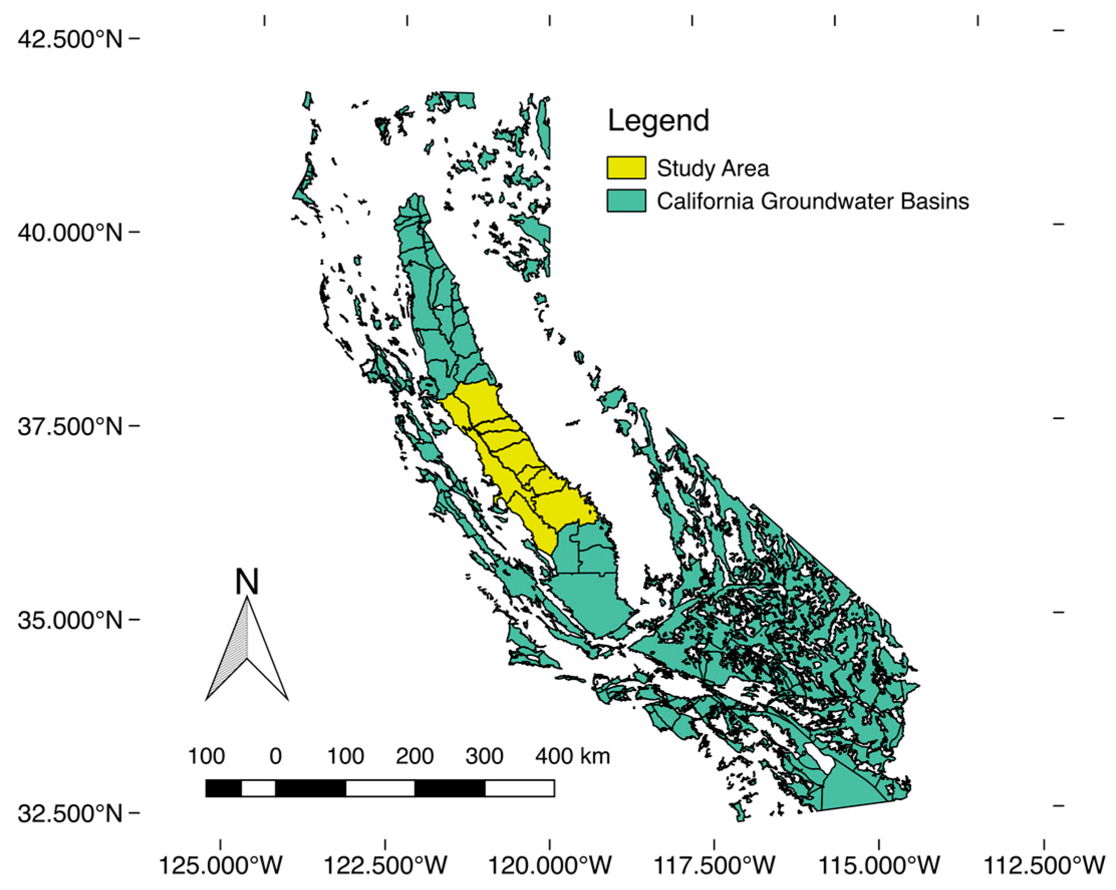
2. Study Region: California’s Central Valley

In California’s Central Valley (see Figure 1), where agricultural water use accounts for one-fifth of the nationwide demand for groundwater, groundwater levels have been declining dramatically over the past few decades [2]. Dependence on groundwater resources is even more pronounced during times of drought as communities and farmers have few alternatives to meet their water needs [59]. In many areas of the Central Valley, the intensive overuse of and reliance on groundwater resources has resulted in land subsidence, degraded water quality, and increasing costs of extraction due to deepening water tables [3,59]. Studies have revealed that the region lost 100 km³ of groundwater since the 1960s [3]. Between 2003 and 2010, GRACE satellite observations showed that the Central Valley lost 20.3 km³ of groundwater, primarily due to extensive groundwater pumping to support agriculture [18]. Dire drought conditions that began in 2011 have caused additional water losses of approximately 10 km³ of freshwater between 2012 and 2013 [22]. From 2012 to present, land subsidence within the Central Valley, which is the result of water loss and compacting sediments within an aquifer, reached up to 280 mm in some places [3]. Another estimate shows that peak rates of subsidence—500 mm/year—occurred during 2014 [3,60].

Despite these dramatic physical impacts to Central Valley aquifers, a comprehensive assessment of California groundwater basins has not been performed since 1980 [62]. The California Department of Water Resources (DWR) cites the lack of information to properly quantify groundwater overdraft as the main reason for this gap in analysis [62]. This is not unique to California. Calls by scientists, engineers, and water managers for more extensive monitoring networks that provide better information for water management have been commonplace throughout the 20th century and still continue to be so today [1].

Ongoing drought conditions, continued groundwater losses, and dramatic rates of land subsidence all point to the need for effective management and heightened monitoring of California’s groundwater resources [59]. GRACE observations provide comprehensive information on drought impacts, climate change, and groundwater and have proven to be a powerful tool for understanding regional water resources behavior [25]. Results from GRACE-based studies have already been used to inform decision-making processes in California’s Central Valley, Texas, and the American Southeast [63]. Refining GRACE to higher resolution estimates of groundwater changes would provide a significant value-added to groundwater management efforts and upcoming implementation of California’s Sustainable Groundwater and Management Act (SGMA) [64].

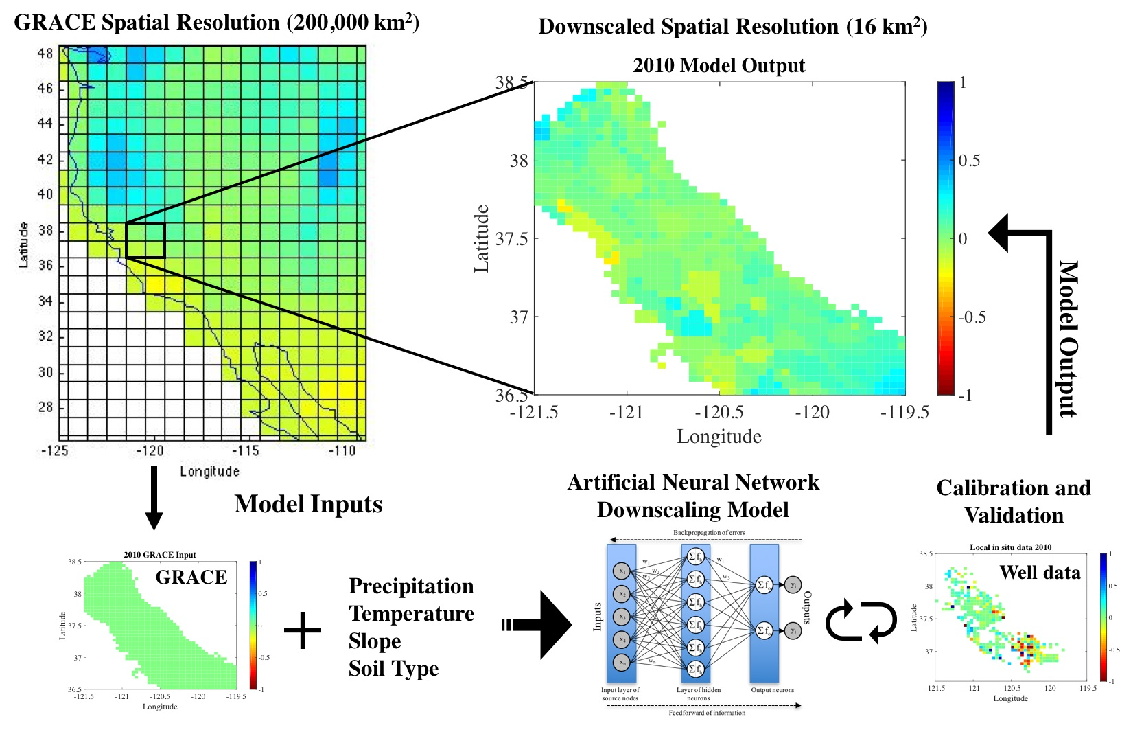
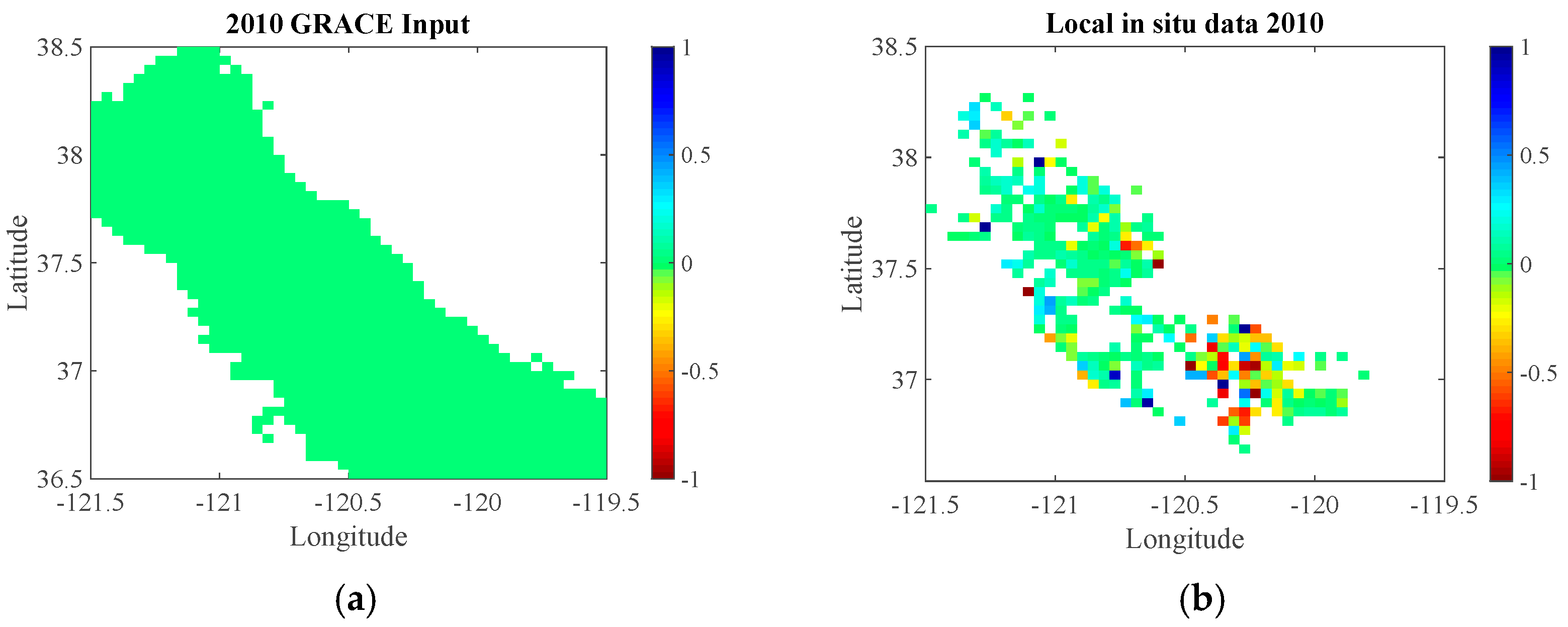
3. The Neural Network Approach and Input Data

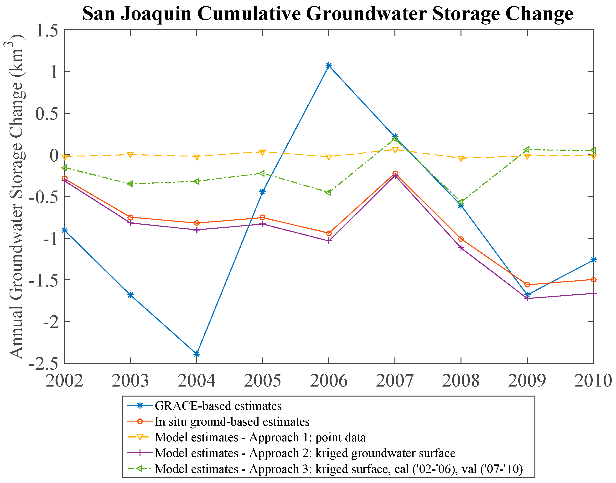
The GRACE downscaling model employs an artificial neural network (ANN) to combine low-resolution GRACE data with higher resolution hydrologic variables in order to predict changes in local groundwater storage and to, in effect, vertically isolate the groundwater component of the GRACE signal. ANNs are particularly useful for this task as they are often employed in spatial data analysis and offer the ability to efficiently and comprehensively handle large, diverse, and noisy spatial datasets [56]. Because they are not yet widely used in statistical downscaling of remote sensing data, this research also represents a novel application of ANNs.

In essence, the ANN derives non-linear, empirical relationships between GRACE, the input hydrologic datasets to the downscaling model, and the output variable—groundwater storage change. These relationships are represented statistically by a network of empirical equations that are fit during the network learning, or calibration, process. Our downscaling model employs a two-layer feed forward neural network, which was calibrated with a Bayesian regularization back propagation learning algorithm [56,65]. A more complete discussion on the training algorithm and neural network architecture can be found in [56,66], respectively.

Because neural networks are data-driven models, the quality and nature of the data used as inputs are of critical importance. Previous studies that employed neural networks to predict groundwater levels utilized both environmental and hydrologic variables and included distinct combinations of: precipitation, temperature, surface discharge (in riparian groundwater systems), tidal levels (in coastal aquifers), and potential evapotranspiration [47,49,50,67]. This study extends this work to focus on storage change rather than groundwater levels. To do so, we use precipitation and temperature data along with GRACE and other key local hydrogeologic datasets (soil type and slope) that are shown in the literature to be significant predictors of terrestrial water storage change [68]. Together, these variables—GRACE observations of terrestrial water storage, slope, soil type, precipitation, and temperature—serve as the hydrologic input data to the neural network model, which is calibrated to changes in in situ groundwater storage. Once calibrated, the downscaling model utilizes the fit empirical relationships between these datasets to generate new estimates of changes in aquifer storage from an alternate set of hydrologic input data from either a new region or from a different point in time. Because the model is calibrated to changes in storage from groundwater alone, the downscaling model also vertically isolates the groundwater component of the GRACE input data. While some studies have modeled or estimated GRACE data input errors [69], it is uncommon in neural network studies [70,71]. As such, we do not address the impact of input errors on model outputs in this work.

Hydrologic datasets used as model inputs were obtained from the 2002–2010 period over California’s Central Valley. They include: annual 2.5 min (~4 km) resolution precipitation and annual mean temperature data from PRISM [72]; static 10-m DEM [73], processed in ArcGIS for percent slope; static 10-m Natural Resources Conservation Service (NRCS) soil maps from the Gridded Soil Survey Geographic (gSSURGO) Database, with 118 different soil types that were coded as dummy variables [74]. All input data were discretized to the 4 km × 4 km target spatial resolution.

GRACE Release 5 (R05) data compiled and processed by the Center for Space Research (CSR) for the period 2002–2010 were used as model inputs and can be found at http://grace.jpl.nasa.gov/data/get-data/monthly-mass-grids-land/. These data consist of monthly measurements across the land surface at a 1-degree × 1-degree resolution. Each grid was multiplied by its scale factor, as provided by GRCTellus, in order to adjust for attenuation of the signal during smoothing and destriping. This procedure is outlined in [75]. Next, each GRACE grid cell in the study region was discretized and spatially interpolated to the target 4 km resolution. To do this, the original GRACE grid cell value was treated as the centroid of the new 4 km discretized grid cell and was interpolated to the centroid of each of the neighboring GRACE grid cell values. A linear interpolation was performed to fill in the rest of the discretized grid between the centroid GRACE value and the values at the corner points. In this way, GRACE data were treated as a surface, taking into account not only a single grid cell but also its neighbors. This allowed the model to incorporate more information about the spatial distribution of groundwater change, rather than just considering a single magnitude. To annualize the GRACE data and make it comparable to the in situ groundwater data, the storage change for twelve months of each year, starting in February, were summed to obtain an annual storage change value.

The groundwater data that serves as the calibration and validation datasets for the neural network model were taken from 2189 wells across San Joaquin County [76]. This dataset can be accessed at http://www.water.ca.gov/waterdatalibrary/. It is important to note that region covered by the model domain, as shown in Figure 1, includes the eleven groundwater sub-basins of the San Joaquin Valley Groundwater Basin and encompasses an area of 15,100 km² [77]. In general, the basin’s hydrogeology is characterized by unconsolidated alluvium and consolidated rocks and includes both confined and unconfined aquifers [77]. The presence of a Corcoran Clay confining layer in most of the Central Valley indicates the transition from unconfined to confined aquifers [2]. Across the study region, hydrogeological studies have shown that most confined aquifers begin at a depth of over 60 m [78,79]. The depth of most of the wells in the dataset ranged between 10 and 25 m, with very few wells at a depth of over 45 m and less than 4% over 60 m. Because nearly all wells tapped unconfined aquifers, groundwater storage change for each well was calculated using a specific yield of 10%, which was reported as the average value for the San Joaquin Valley by the USGS [80]. The specific yield was multiplied by annual groundwater level change, calculated as the difference in well levels from one year to the next, using winter (December–February) as an annual reference point. This assured the capture of the full irrigation season in a given year, as groundwater abstraction is the key driver of storage change in this region. A more specific description on the complex hydrogeology of the individual sub-basins can be found in California’s Department of Water Resources Bulletin 118 basin descriptions: http://www.water.ca.gov/groundwater/bulletin118/.

The neural network downscaling approach reduces some of the hydrogeological complexity found in the natural system, as we do not directly include any hydrogeological data on these multiple aquifer systems. The model, instead, relies on empirical relationships derived between groundwater change behavior and the input datasets (GRACE, precipitation, temperature, slope, and soil type). These empirical relationships, which vary across space and time, reflect not only temporal and spatial trends in extraction, they also represent the physical characteristics of the multiple aquifer systems, due to their grounding in location-specific in situ datasets.

The calibration and validation data were formatted in two ways for the neural network—distributed point data and spatially interpolated maps of the study region, as shown in Figure 2. The distributed point dataset was obtained by directly applying the groundwater storage change estimates to a 4 km grid of the region based on each wells latitude and longitude. If more than one well fell within a given grid cell, the average of all wells was used. The spatially interpolated groundwater storage change maps were created by kriging the individual groundwater storage change estimates, as this approach has been found to best approximate groundwater spatially [12,81]. A more complete discussion on the kriging methodology can be found in [82], and its applicability to represent characteristics of multiple aquifer systems can be found in [83]. More specifically, ordinary kriging was applied to groundwater well data points using an empirically fit spherical semivariogram with a 300 m nugget, a similar value to regional kriging approaches employed in the San Joaquin basin [2]. Spherical semivariograms are commonly used with ordinary kriging, and the choice of semivariogram is often determined empirically. In this case, a spherical semivariogram resulted in the lowest mean error, average standard error, and root mean square error when compared to pentaspherical and exponential semivariograms. We followed the procedures outlined in [84,85] for semivariogram selection. One kriged map was created for each year. The annual change in groundwater storage, rather than the water levels themselves, was used to create a comparable dataset to the GRACE data, which reflects variations in water storage. In this way, both GRACE and the groundwater data both represented a monthly height difference in water storage.

4. Results

The results are divided according to the calibration data type and validation approach used. Calibration and validation of the neural network model were performed with two data types—distributed point data and spatially interpolated maps of the study region. The model was then validated either on a spatial subset of the data within a given year (50% of the original dataset) or was validated on the entire spatial dataset but for a temporal subset of a range years (2007–2010). More specifically, the first calibration method uses annual groundwater storage changes from individual wells in each year (2002–2010) for calibration and validates the model over a subset of groundwater storage changes in each year. These in situ data remain spatially discrete points. The second method, by contrast, uses spatially interpolated groundwater storage changes, e.g., groundwater maps, in each year (2002–2010) for calibration and validates the model over a subset of the in situ data that is randomly selected in each year. This subset is kriged separately following the same procedures to insure data independence. The final method uses spatially interpolated groundwater maps for calibration for 2002–2006 and validates the model over the years 2007–2010 across the entire spatial region. Each calibration and validation dataset is selected randomly from the total sample. By analyzing these approaches, we are able to determine what type of calibration and validation data best informs the network and improves its performance. The performance of each approach was assessed through the use of various model evaluation statistics (Nash–Sutcliffe model efficiency coefficient, root mean squared error, correlation coefficient) and measures of the spatial distribution of model error (relative error, absolute error) [86].

In order to quantify the relative contribution of each input dataset onto the neural network model output, we applied Garson’s method [87]. Garson’s method is based on the weights of the calibrated neural network and has been widely cited and is widely used in neural network studies [88,89,90,91]. This method identifies the percentages of influence, ${\mathit{Q}}_{\mathit{i}\mathit{k}}(\%)$, of each of the input variables on the model’s prediction of the output variable [87,88]. It is defined by the following equation:

$${\mathit{Q}}_{\mathit{i}\mathit{k}}(\%)= \frac{{{\displaystyle \sum }}_{\mathit{j}=\mathbf{1}}^{\mathit{n}}\left(\frac{\left|{\mathit{w}}_{\mathit{i}\mathit{j}}\right|}{{{\displaystyle \sum }}_{\mathit{i}=\mathbf{1}}^{\mathit{m}}\left|{\mathit{w}}_{\mathit{i}\mathit{j}}\right|}\left|{\mathit{v}}_{\mathit{j}\mathit{k}}\right|\right)}{{{\displaystyle \sum }}_{\mathit{i}=\mathbf{1}}^{\mathit{m}}\left({{\displaystyle \sum }}_{\mathit{j}=\mathbf{1}}^{\mathit{n}}\left(\frac{\left|{\mathit{w}}_{\mathit{i}\mathit{j}}\right|}{{{\displaystyle \sum }}_{\mathit{i}=\mathbf{1}}^{\mathit{m}}\left|{\mathit{w}}_{\mathit{i}\mathit{j}}\right|}\left|{\mathit{v}}_{\mathit{j}\mathit{k}}\right|\right)\right)}\times 100$$

(1)

where ${\mathit{w}}_{\mathit{i}\mathit{j}}$ represents the weights between the input variables (neurons), $\mathit{i}=\mathbf{1}, \mathbf{2},\mathbf{\dots }\mathit{m},$ and each of the two hidden layers, $\mathit{j}=\mathbf{1}, \mathbf{2}\mathbf{\dots }\mathit{n}; {\mathit{v}}_{\mathit{j}\mathit{k}}$ represents the weights between the hidden layers and the output variable (neuron), $\mathit{k}=\mathbf{1}, \mathbf{2},\mathbf{\dots }\mathit{l}$; and the number of input neurons, hidden layers, and output neurons were $\mathit{m}=\mathbf{5}, \mathit{n}=\mathbf{2}, \mathit{l}=\mathbf{1}$, respectively. The number of output neurons is equivalent to the number of grid cells being simulated. Each model has two hidden layers with 122 neurons each. The results of this method are shown and discussed below in Section 4.4.

4.1. Approach 1: In Situ Point Data for Calibration

The first approach calibrates the model with annual groundwater storage changes from each available grid cell in each year (2002–2010). In this approach, 50 percent of the available well information in a given year was selected randomly from the dataset and used for calibration, and the remaining 50 percent was set aside for validation of the model. Results are shown below in

Table 1. Results of neural network downscaling approach with uninterpolated points for calibration (50% calibration, 50% validation).

Year	Calibration Results			Validation Results
	NSE	Corr. Coeff.	RMSE (m)	NSE	Corr. Coeff.	RMSE (m)
2002	0.5185	0.1665	0.0512	0.1435	0.1222	0.0586
2003	0.8731	0.2543	0.1210	0.4831	0.3098	0.1061
2004	0.3555	0.3578	0.1036	0.1569	0.3397	0.0845
2005	0.3603	0.2745	0.0814	0.0967	0.2397	0.0941
2006	0.2683	0.1566	0.0861	0.0683	0.1770	0.1200
2007	0.1580	0.4180	0.5608	0.5851	0.2489	0.1044
2008	0.8732	0.2189	0.1215	0.2977	0.2211	0.1263
2009	0.8152	0.2340	0.1159	0.0773	0.1426	0.1466
2010	0.0448	0.1749	0.0853	0.1676	0.0818	0.1099

. From Table 1, we can see that Nash-Sutcliffe efficiency (NSE) values for validation mostly fall within the acceptable range (0–1), but the correlation between simulated and observed values is fairly low. Visual inspection of the spatial distribution of simulated groundwater data also performed poorly, as little to no heterogeneity in the spatial pattern was visible. For these reasons, this approach does not fully capture groundwater behavior across space and during the time period of study.

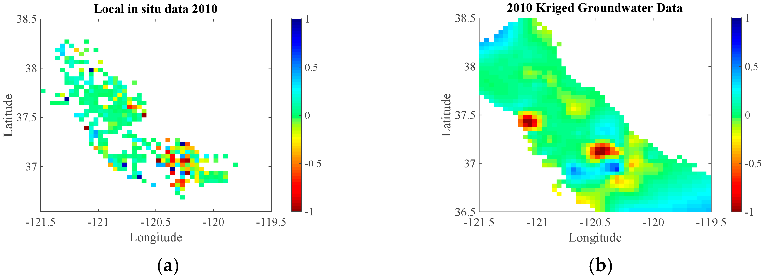
4.2. Approach 2: Kriged Groundwater Surface for Calibration

The second approach to the neural network validation and calibration used a spatially interpolated (kriged) groundwater dataset. Similar to the first approach, 50 percent of the kriged groundwater data was used for calibration, and the remaining portion of the dataset (50 percent) was used to validate the model. By calibrating the model to a best guess of the groundwater surface in the region as opposed to sparse point data, we provided more information to the neural network during the calibration process. Note that computational time for each network calibration for each year was an average of approximately 4 min, accounting for data preprocessing and kriging.

Table 2. Results of neural network downscaling approach with a kriged groundwater surface for calibration (50% calibration, 50% validation).

Year	Calibration Results			Validation Results
	NSE	Corr. Coeff.	RMSE (m)	NSE	Corr. Coeff.	RMSE (m)
2002	0.8364	0.9146	0.0266	0.3981	0.6359	0.0610
2003	0.9431	0.9717	0.0800	0.7511	0.8907	0.2390
2004	0.5624	0.7502	0.0754	0.0692	0.5227	0.3698
2005	0.6976	0.8393	0.0414	0.3185	0.5798	0.1326
2006	0.5799	0.7604	0.0511	0.0453	0.1602	0.0818
2007	0.6111	0.7826	0.3772	0.2096	0.3102	0.6236
2008	0.9577	0.9787	0.0690	0.3285	0.7219	0.2114
2009	0.8721	0.9365	0.1236	0.0391	0.7560	0.1924
2010	0.2445	0.4966	0.0541	0.2547	0.4843	0.0519

shows error indicators of model results. This approach produced acceptable NSE values (ranging from 0.2445 to 0.9577) for calibration and validation (ranging from 0.0391 to 0.7511), indicating that the model’s simulated values are better predictors than observed values alone [92]. From Table 2, it is also evident that the model results have a high degree of correlation to the calibration and validation datasets.

Figure 3 illustrates the modeled spatial distribution of groundwater change in 2010 along with the absolute and relative errors between groundwater calibration data and model outputs. The error maps show that the majority of the absolute and relative error is close to zero (shown in green). In addition, there is little spatial bias in model error; however, most of the error does correspond to areas of more extreme values, indicating that the model’s ability to predict extrema (peak and troughs) may be limited.

4.3. Approach 3: Kriged Groundwater Surface for Calibration (2002–2006) with Validation over Entire Surface (2007–2010)

The final approach for calibration and validation of the neural network model utilized the same spatially interpolated (kriged) dataset from the second approach but validated the model over four annual time periods (2007–2010) rather than on a portion of the data within each year. In this case, calibration of the neural network model was performed over the first set of years (2002–2006).

Table 3. Results of neural network downscaling approach with a kriged groundwater surface for calibration.

Calibration (2002–2006), Validation (2007–2010)
Year	NSE	Corr. Coeff.	RMSE (m)
2002	0.5509	0.7429	0.0240
2003	0.8752	0.9355	0.0673
2004	0.6887	0.8302	0.0582
2005	0.8360	0.9143	0.0471
2006	0.6839	0.8270	0.0479
2007	−0.1029	0.1772	0.5246
2008	−3.7980	0.1965	0.6708
2009	−0.3598	0.2301	0.1605
2010	−0.0029	0.3048	0.0642

shows the overall performance and error indicators of model output. We can see that again NSE values fall in the acceptable range for calibration but are outside of this range for the validation time periods. Further visual inspection of the spatial distribution of both absolute error and relative error for this modeling approach shows significantly more error than in the second approach.

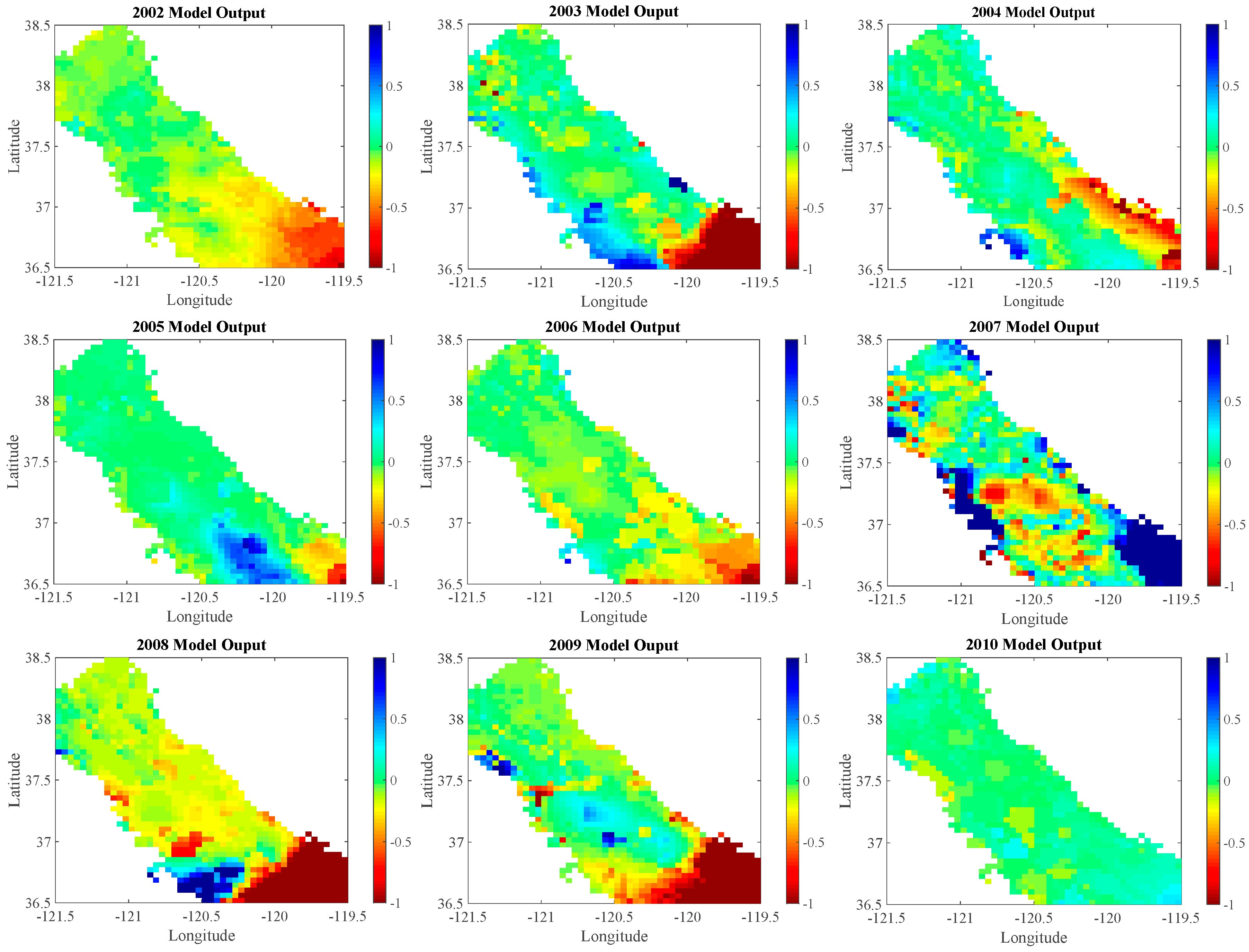
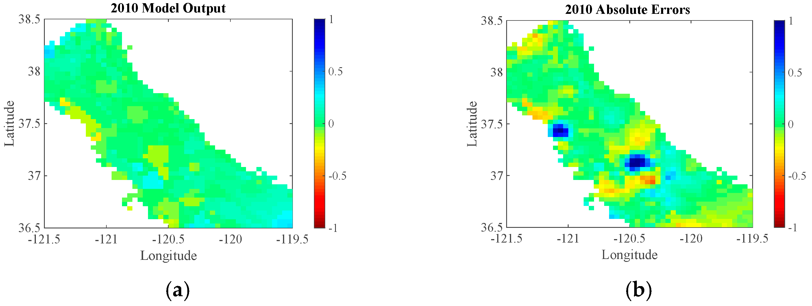
4.4. Finalized Neural Network Model Results

The output data of the neural network model contained the least error and highest correlations when using the second approach. Because the model was unsuccessful in simulating groundwater change in new time periods, it is clear that the model requires some groundwater information as an input. This also highlights one of the limitations of an empirically based downscaling model—once calibrated to a particular period of time or location in space, the model may not accurately represent the groundwater changes in a new region or time period. However, following the second approach, which calibrates each year to a widely available interpolated set of groundwater storage change, the proposed model can acceptably simulate the groundwater surface and downscale GRACE data to the 4 km resolution. The maps shown below in Figure 4 are the final output of the model. Error data for these maps can be found in Table 2.

From Figure 4, we can see that the large majority of the groundwater declines (shown in red) during the 2002–2010 time period in California’s Central Valley occurred in the eastern and southern portions of the southern Central Valley. These hotspots of groundwater depletion show up to 1 m of storage loss per unit area in some locations of the southern and eastern portions of the study region. Madera, for example, is located at 36.956476, −120.051041 and shows between 0.25 and 1 m of groundwater storage loss in all years except 2007. Other areas, shown in greens and blues, experienced relative increases in groundwater storage. These locations varied from year to year. The central portions of the southern end of the map had recurring increases in the groundwater table (see years 2003, 2005, and 2009). Further study of this region could be complemented with the use of high-resolution groundwater models to help elucidate why and how certain regions may be losing or gaining groundwater.

Overall, the model output maps point to a high degree of heterogeneity in groundwater behavior compared to GRACE data. As such, it is critical to keep in mind the increase in resolution these maps provide. Figure 5 below shows the resolution of the GRACE estimates of total water storage and currently available groundwater well data for this region in 2010. Looking at the GRACE data in Figure 5, we can see a slight average regional increase in groundwater storage. However, the model output from this study shows that at a more local level, groundwater may be exhibiting more dramatic increases and decreases. These extrema are more or less averaged out at such a low spatial resolution seen in GRACE data. The in situ groundwater data shown in Figure 5 does capture some of these highs and lows but fails to provide adequate spatial coverage.

Figure 6 shows the percent by which each input variable influences the model output, as calculated from Equation (1), in our final neural network model. GRACE has the highest percent influence (PI) on model output, 38.76%, followed by precipitation, 21.99%, temperature, 15.54%, slope, 12.41%, and soil type, 11.30%. These values illustrate that GRACE is able to explain a significant portion of groundwater storage change in the San Joaquin portion of the Central Valley. Because GRACE only provides low spatial resolution information, the PI values also show that the remaining input variables are necessary to achieve model output at our target, higher spatial resolution.

A time series of cumulative groundwater storage change over the 2002–2010 study period is shown in Figure 7 as estimated from the three model approaches, from in situ data and from GRACE estimates of changes in total water storage. The comparison of the two time series shows that in some years, GRACE appears to be overestimating annual storage loss (2002–2004) and gain (2006) in this region. This may be due to gaps in the spatial coverage of well data, where significant groundwater pumping may be occurring. It could also be the result of surface water storage dynamics, as GRACE also detects changes in surface water. In addition, the model output may be underestimating the groundwater change due to errors in the spatial interpolation methodology. The actual annual change is most likely somewhere between the two lines.

5. Discussion

Overall, the model output demonstrates that when remote sensing and monitoring data are used together, as in our neural network model, they are able to provide a clearer picture of local and regional groundwater patterns than the use of each data type in isolation (shown in Figure 5). Our results show that our neural network downscaling model effectively simulates groundwater storage change and downscale GRACE data to a 4 km resolution. While we were able to generate high-resolution groundwater maps for the central and southern portions of the Central Valley, our modeling approach was unsuccessful in simulating groundwater change in new time periods or over new spatial domains. Thus, one of the limitations of our empirically based model is that, once calibrated, the model may not accurately represent the groundwater changes in a region or time period outside of the calibration domain.

One of the advantages of our neural network downscaling model is that it is model-independent and computationally flexible. The comparison of the high-resolution maps generated in this study to the output from regional physics-based groundwater models could, however, further confirm or improve the effectiveness of this method. In addition, a deeper analysis of the implications of the findings in this study to local groundwater management would be highly beneficial for groundwater managers.

Further, the extension of GRACE data by means of statistical downscaling represents a unique contribution to the scientific remote sensing community and advances the state of current remote sensing-based hydrologic science. This approach departs from data assimilation methods in that it is model-independent and thus offers more flexibility in data scarce environments and with changing input data products (i.e., new data releases or alternate remote sensing products). This has implications for world-wide applicability in developing regions, where models and dense monitoring networks may not be freely available. This neural network model also constitutes an alternative, statistical approach to improving the resolution of remote sensing products and offers a hybrid solution between low-resolution GRACE data and sparse groundwater monitoring networks.

6. Conclusions

Sustainable planning and management of groundwater resources requires accurate information about trends in groundwater availability. GRACE has already proven to be a powerful data source for regional groundwater assessments in many areas around the world, yet its applicability to more localized studies and its utility to water management authorities have been constrained by its limited spatial resolution (~200,000 km²) [25,93]. We developed a robust, artificial neural network model that downscales GRACE gridded land datasets (~1 degree) to higher-resolution (~4 km) groundwater storage change estimates. The model utilized GRACE estimates of variations in total water storage and a series of widely available hydrologic variables (PRISM precipitation and temperature data, DEM-derived slope, and NRCS soil type) to derive spatial patterns in groundwater behavior. The neural network downscaling model was able to effectively simulate groundwater storage change over the central and southern portions of the Central Valley with NSE values ranging from 0.0391 to 0.7511. This study also showed that the model required richer estimations of groundwater data (kriged datasets) for improved calibration and validation performance. The results of the downscaling model—high-resolution maps of groundwater storage change—illustrated the high heterogeneity in groundwater behavior and the tendency for more dramatic declines in the groundwater table to occur in the southern and western portions of the San Joaquin Valley and Tulare Groundwater Basins.

References

1. Taylor, C.; Alley, W. Ground-Water-Level Monitoring and the Importance of Long-Term Water-Level Data; USGS Circular 1217; USGS: Reston, VA, USA, 2001. Available online: http://pubs.usgs.gov/circ/circ1217/pdf/circular1217.pdf (accessed on 20 August 2017).
2. Faunt, C. Groundwater Availability of the Central Valley Aquifer, California; USGS Professional Paper 1766; USGS: Reston, VA, USA, 2009. Available online: http://pubs.usgs.gov/pp/1766/ (accessed on 20 August 2017).
3. Faunt, C.; Sneed, M. Water Availability and Subsidence in California’s Central Valley. San Franc. Estuary Watershed Sci. 2015, 13. Available online: http://escholarship.org/uc/item/6qn2711x (accessed on 20 August 2017). [CrossRef]
4. Mogheir, Y.; De Lima, J.L.M.P.; Singh, V.P. Assessment of Informativeness of Groundwater Monitoring in Developing Regions (Gaza Strip Case Study). Water Resour. Manag. 2005, 19, 737. [Google Scholar] [CrossRef]
5. Shah, T.; Molden, D.; Sakthivadivel, R.; Seckler, D. The Global Groundwater Situation: Overview of Opportunities and Challenges; International Water Management Institute: Colombo, Sri Lanka, 2000; Available online: http://publications.iwmi.org/pdf/H025885.pdf (accessed on 20 August 2017).
6. Harbaugh, A.; Banta, E.; Hill, M.; McDonald, M. MODFLOW-2000, the U.S. Geological Survey Modular Ground-Water Model—User Guide to Moduralization Concepts and the Ground-Water Flow Process; USGS: Reston, VA, USA, 2000. Available online: https://pubs.usgs.gov/of/2000/0092/report.pdf (accessed on 20 August 2017).
7. Dagan, G. Stochastic modeling of groundwater flow by unconditional and conditional probabilities: 1. Conditional simulation and the direct problem. Water Resour. Res. 1982, 18, 813–833. [Google Scholar] [CrossRef]
8. Hendricks Franssen, H.J.; Kinzelbach, W. Real-time groundwater flow modeling with the Ensemble Kalman Filter: Joint estimation of states and parameters and the filter inbreeding problem. Water Resour. Res. 2008, 44. [Google Scholar] [CrossRef]
9. Reed, P.; Minsker, R.; Valocchi, A. Cost-effective long-term groundwater monitoring design using a genetic algorithm and global mass interpolation. Water Resour. Res. 2000, 36, 3731–3741. [Google Scholar] [CrossRef]
10. Hughes, J.; Lettenmaier, D. Data requirements for kriging: Estimation and network design. Water Resour. Res. 1981, 17, 1641–1650. [Google Scholar] [CrossRef]
11. Kitanidis, P.; Vomvoris, E. A geostatistical approach to the inverse problem in groundwater modeling (steady state) and one-dimensional simulations. Water Resour. Res. 1983, 19, 677–690. [Google Scholar] [CrossRef]
12. Sun, Y.; Kang, S.; Li, F.; Zhang, L. Comparison of interpolation methods for depth to groundwater and its temporal and spatial variations in the Minqin oasis of northwest China. Environ. Model. Softw. 2009, 24, 1163–1170. [Google Scholar] [CrossRef]
13. Rodell, M.; Famiglietti, J.S. The potential for satellite-based monitoring of groundwater storage changes using GRACE: The High Plains aquifer, Central US. J. Hydrol. 2003, 263, 245–256. [Google Scholar] [CrossRef]
14. Yeh, P.; Swenson, S.; Famiglietti, J.S.; Rodell, M. Remote sensing of groundwater storage changes in Illinois using the Gravity Recovery and Climate Experiment (GRACE). Water Resour. Res. 2009, 42. [Google Scholar] [CrossRef]
15. Rodell, M.; Chen, J.; Kato, H.; Famiglietti, J.S.; Nigro, J.; Wilson, C.R. Estimating groundwater storage changes in the Mississippi River basin (USA) using GRACE. Hydrogeol. J. 2007, 15, 159–166. [Google Scholar] [CrossRef]
16. Strassberg, G.; Scanlon, B.; Rodell, M. Comparison of seasonal terrestrial water storage variations from GRACE with groundwater-level measurements from the High Plains Aquifer (USA). Geophys. Res. Lett. 2007, 34. [Google Scholar] [CrossRef]
17. Rodell, M.; Velicogna, I.; Famiglietti, J.S. Satellite-based estimates of groundwater depletion in India. Nature 2009, 460, 999–1002. [Google Scholar] [CrossRef] [PubMed]
18. Famiglietti, J.S.; Lo, M.; Ho, S.L.; Bethune, J.; Anderson, K.; Syed, T.; Swenson, S.; de Linage, C.; Rodell, M. Satellites measure recent rates of groundwater depletion in California’s Central Valley. Geophys. Res. Lett. 2011, 38, L03403. [Google Scholar] [CrossRef]
19. Munier, S.; Becker, M.; Maisongrande, P.; Cazenave, A. Using GRACE to detect Groundwater Storage variations: The cases of Canning Basin and Guarani Aquifer System. Int. Water Technol. J. 2012, 2, 2–13. [Google Scholar]
20. Voss, K.; Famiglietti, J.S.; Lo, M.; de Linage, C.; Rodell, M.; Swenson, S.C. Groundwater depletion in the Middle East from GRACE with implications for transboundary water management in the Tigris-Euphrates-Western Iran region. Water Resour. Res. 2013, 49, 904–914. [Google Scholar] [CrossRef] [PubMed]
21. Feng, W.; Zhong, M.; Lemoine, J.M.; Biancale, R.; Hsu, H.T.; Xia, J. Evaluation of groundwater depletion in North China using the Gravity Recovery and Climate Experiment (GRACE) data and ground-based measurements. Water Resour. Res. 2013, 49, 2110–2118. [Google Scholar] [CrossRef]
22. Famiglietti, J.S. The global groundwater crisis. Nat. Clim. Chang. 2014, 4, 945–948. [Google Scholar] [CrossRef]
23. Richey, A.S.; Thomas, B.F.; Lo, M.H.; Reager, J.T.; Famiglietti, J.S.; Voss, K.; Swenson, S.; Rodell, M. Quantifying renewable groundwater stress with GRACE. Water Resour. Res. 2015, 51, 5217–5238. [Google Scholar] [CrossRef] [PubMed]
24. Richey, A.S.; Thomas, B.F.; Lo, M.H.; Famiglietti, J.S.; Swenson, S.; Rodell, M. Uncertainty in global groundwater storage estimates in a Total Groundwater Stress framework. Water Resour. Res. 2015, 51, 5198–5216. [Google Scholar] [CrossRef] [PubMed]
25. Famiglietti, J.S.; Rodell, M. Water in the balance. Science 2013, 340, 1300–1301. [Google Scholar] [CrossRef] [PubMed]
26. Alley, W.M.; Konikow, L.F. Bringing GRACE Down to Earth. Groundwater 2015, 53, 826–829. [Google Scholar] [CrossRef] [PubMed]
27. Fekete, B.M.; Robarts, R.D.; Kumagai, M.; Nachtnebel, H.P.; Odada, E.; Zhulidov, A.V. Time for in situ renaissance. Science 2015, 349, 685–686. [Google Scholar] [CrossRef] [PubMed]
28. Wilby, R.L.; Wigley, T.M.L. Downscaling general circulation model output: A review of methods and limitations. Prog. Phys. Geogr. 1997, 21, 530–548. [Google Scholar] [CrossRef]
29. Zaitchik, B.; Rodell, M.; Reichle, R. Assimilation of GRACE Terrestrial Water Storage Data into a Land Surface Model: Results for the Mississippi River Basin. J. Hydrometeorol. 2008, 9, 535–548. [Google Scholar] [CrossRef]
30. Schumacher, M.; Forootan, E.; van Dijk, A.I.J.M.; Müller Schmied, H.; Crosbie, R.S.; Kushche, J.; Döll, P. Improving drought simulations within the Murray-Darling Basin by combined calibration/assimilation of GRACE data into the WaterGAP Global Hydrology Model. Remote Sens. Environ. 2017, 204, 212–228. [Google Scholar] [CrossRef]
31. Schoof, J. Statistical Downscaling in Climatology. Geogr. Compass 2013, 7, 249–265. [Google Scholar] [CrossRef]
32. Wilby, R.L.; Wigley, T.M.L.; Conway, D.; Jones, P.D.; Hewitson, B.C.; Main, J.; Wilks, D.S. Statistical downscaling of general circulation model output: A comparison of methods. Water Resour. Res. 1998, 34, 2995–3008. [Google Scholar] [CrossRef]
33. Forootan, E.; Rietbroek, R.; Kusche, J.; Sharifi, M.A.; Awange, J.L.; Schmidt, M.; Omondi, P.; Famiglietti, J. Separation of large scale water storage patterns over Iran using GRACE, altimetry and hydrological data. Remote Sens. Environ. 2014, 140, 580–595. [Google Scholar] [CrossRef]
34. Wilby, R.L.; Charles, S.P.; Zorita, E.; Timbal, B.; Whetton, P.; Mearns, L.O. Guidelines for Use of Climate Scenarios Developed from Statistical Downscaling Methods. Task Group of Data and Scenario Support for Impacts and Climate Analysis (TGICA). Intergovernmental Panel on Climate Change. 2004. Available online: http://www.ipcc-data.org/guidelines/dgm_no1_v1_10-2003.pdf (accessed on 20 August 2017).
35. Huang, H.Y.; Capps, S.; Huang, S.C.; Hall, A. Downscaling near-surface wind over complex terrain using a physically-based statistical modeling approach. Clim. Dyn. 2015, 44, 529–542. [Google Scholar] [CrossRef]
36. Chiew, F.; Kirono, D.; Kent, D.; Frost, A.; Charles, S.P.; Timbal, B.; Nguyen, K.; Fu, G. Comparison of runoff modelled using rainfall from different downscaling methods for historical and future climates. J. Hydrol. 2010, 387, 10–23. [Google Scholar] [CrossRef]
37. Fasbender, D.; Ouarda, T. Spatial Bayesian Model for Statistical Downscaling of AOGCM to Minimum and Maximum Daily Temperatures. J. Clim. 2010, 23, 5222–5242. [Google Scholar] [CrossRef]
38. Frost, A.; Charles, S.; Timbal, B.; Chiew, F.; Mehrotra, R.; Nguyen, K.; Chandler, R.; McGregor, J.; Fu, G.; Kirono, D.; et al. A comparison of multi-site rainfall downscaling techniques under Australian conditions. J. Hydrol. 2011, 408, 1–18. [Google Scholar] [CrossRef]
39. Schoof, J.; Pryor, S.C. Downscaling temperature and precipitation: A comparison of regression-based methods and artificial neural networks. Int. J. Climatol. 2001, 21, 773–790. [Google Scholar] [CrossRef]
40. Dibike, Y.; Coulibaly, P. Temporal neural networks for downscaling climate variability and extremes. Neural Netw. 2006, 19, 135–144. [Google Scholar] [CrossRef] [PubMed]
41. Fowler, H.J.; Blenkinsop, S.; Tebaldi, C. Linking climate change modelling to impacts studies: Recent advances in downscaling techniques for hydrological modeling. Int. J. Climatol. 2007, 27, 1547–1578. [Google Scholar] [CrossRef]
42. French, M.; Krajewski, W.; Cuykendall, R. Rainfall forecasting in space and time using a neural network. J. Hydrol. 1992, 137, 1–31. [Google Scholar] [CrossRef]
43. Zhu, A. Mapping soil landscape as spatial continua: The Neural Network Approach. Water Resour. Res. 2000, 36, 663–677. [Google Scholar] [CrossRef]
44. Jin, L.; Lin, J.; Lin, K. Precipitation Prediction Modeling Using Neural Network and Empirical Orthogonal Function Base on Numerical Weather Forecast Production. In Proceedings of the 6th World Congress on Intelligent Control and Automation, Dalian, China, 21–23 June 2006. [Google Scholar]
45. Chu, H.; Chang, L. Optimal control algorithm and neural network for dynamic groundwater management. Hydrol. Process. 2009, 23, 2765–2773. [Google Scholar] [CrossRef]
46. Daliakopoulos, I.; Coulibaly, P.; Tsanis, I. Groundwater level forecasting using artificial neural networks. J. Hydrol. 2005, 309, 229–240. [Google Scholar] [CrossRef]
47. Krishna, B.; Satyaji Rao, Y.R.; Vijaya, T. Modelling groundwater levels in an urban coastal aquifer using artificial neural networks. Hydrol. Process. 2008, 22, 1180–1188. [Google Scholar] [CrossRef]
48. Yang, Z.; Lu, W.; Long, Y.; Li, P. Application and comparison of two prediction models for groundwater levels: A case study in Western Jilin Province, China. J. Arid Environ. 2009, 73, 487–492. [Google Scholar] [CrossRef]
49. Yoon, H.; Jun, S.C.; Hyun, Y.; Bae, G.O.; Lee, K.K. A comparative study of artificial neural networks and support vector machines for predicting groundwater levels in a coastal aquifer. J. Hydrol. 2011, 396, 128–138. [Google Scholar] [CrossRef]
50. Taormina, R.; Chau, K.; Sethi, R. Artificial neural network simulation of hourly groundwater levels in a coastal aquifer system of the Venice lagoon. Eng. Appl. Artif. Intell. 2012, 25, 1670–1676. [Google Scholar] [CrossRef]
51. Ebrahimi, H.; Rajaee, T. Simulation of groundwater level variations using wavelet combined with neural network, linear regression and support vector machine. Glob. Planet. Chang. 2017, 148, 181–191. [Google Scholar] [CrossRef]
52. Sahoo, S.; Russo, T.A.; Elliott, J.; Foster, I. Machine learning algorithms for modeling groundwater level changes in agricultural regions of the U.S. Water Resour. Res. 2017, 53, 3878–3895. [Google Scholar] [CrossRef]
53. Sun, A. Predicting groundwater level changes using GRACE data. Water Resour. Res. 2013, 49, 5900–5912. [Google Scholar] [CrossRef]
54. Hsu, K.; Goa, X.; Sorooshian, S.; Gupta, H. Precipitation Estimation from Remotely Sensed Information Using Artificial Neural Networks. J. Appl. Meteorol. 1997, 36, 1176–1190. [Google Scholar] [CrossRef]
55. Hsu, K.; Gupta, H.V.; Sorooshian, S. Artificial Neural Network Modeling of the Rainfall-Runoff Process. Water Resour. Res. 1995, 31, 2517–2530. [Google Scholar] [CrossRef]
56. Turban, E.; Sharda, R.; Aronson, J.E.; King, D.N. Business Intelligence: A Managerial Approach; Pearson Prentice Hall: Upper Saddle River, NJ, USA, 2008. [Google Scholar]
57. Wiese, D.N. GRACE Monthly Global Water Mass Grids, NETCDF RELEASE 5.0. Ver. 5.0. PO.DAAC, CA, USA. 2015. Available online: http://grace.jpl.nasa.gov/data/get-data/jpl_global_mascons/ (accessed on 20 August 2017).
58. Jet Propulsion Laboratory, GRACE Follow-On, California Institute of Technology. NASA. 2016. Available online: http://gracefo.jpl.nasa.gov/ (accessed on 20 August 2017).
59. Howitt, R.; MacEwan, D.; Medellín-Azuara, J.; Lund, J.; Sumner, D. Economic Analysis of the 2015 Drought for California Agriculture. UC Davis Center for Watershed Science. 2015. Available online: https://watershed.ucdavis.edu/files/biblio/Final_Drought%20Report_08182015_Full_Report_WithAppendices.pdf (accessed on 20 August 2017).
60. Farr, T.; Jones, C.; Lui, Z. Progress Report: Subsidence in the Central Valley, California, Sacramento (CA): California Department of Water Resources. 2015. Available online: http://water.ca.gov/groundwater/docs/NASA_REPORT.pdf (accessed on 20 August 2017).
61. California Department of Water Resources, California’s Groundwater: Bulletin 118, California Department of Water Resources. 2016. Available online: http://www.water.ca.gov/groundwater/bulletin118/gwbasins.cfm (accessed on 20 August 2017).
62. RMC, An Evaluation of California Groundwater Management Planning, California Water Foundation. Sacramento, CA. 2015. Available online: http://www.californiawaterfoundation.org/uploads/1405009350-GMPReport2014(00256304xA1C15).pdf (accessed on 20 August 2017).
63. Lo, M.; Famiglietti, J.S. Irrigation in California’s Central Valley strengthens the southwestern U.S. water cycle. Geophys. Res. Lett. 2013, 40, 301–306. [Google Scholar] [CrossRef]
64. California Department of Water Resources, Legislation, Sustainable Groundwater Management Act (SGMA), California Department of Water Resources. 2015. Available online: http://www.water.ca.gov/cagroundwater/legislation.cfm (accessed on 20 August 2017).
65. Mathworks, Neural Network Toolbox, MATLAB. 2016. Available online: http://www.mathworks.com/products/neural-network/ (accessed on 20 August 2017).
66. MacKay, D. Bayesian Interpolation. Neural Comput. 1992, 4, 415–447. [Google Scholar] [CrossRef]
67. Lallahem, S.; Mania, J.; Hani, A.; Najjar, Y. On the use of neural networks to evaluate groundwater levels in fractured media. J. Hydrol. 2005, 307, 92–111. [Google Scholar] [CrossRef]
68. Reager, J.T.; Famiglietti, J.S. Characteristic mega-basin water storage behavior using GRACE. Water Resour. Res. 2013, 49, 3314–3329. [Google Scholar] [CrossRef] [PubMed]
69. Güntner, A. Improvement of Global Hydrologic Models Using GRACE Data. Surv. Geophys. 2008, 29, 375–397. [Google Scholar] [CrossRef]
70. Cannon, A.J.; Whitfield, P.H. Downscaling recent streamflow conditions in British Columbia, Canada using ensemble neural network models. J. Hydrol. 2002, 259, 136–151. [Google Scholar] [CrossRef]
71. Basheer, I.A.; Hajmeer, M. Artificial neural networks: Fundamentals, computing, design, and application. J. Microbiol. Methods 2000, 43, 3–31. [Google Scholar] [CrossRef]
72. PRISM Climate Group, PRISM Climate Data, Northwest Alliance for Computational Science and Engineering, Oregon State University. 2014. Available online: http://www.prism.oregonstate.edu (accessed on 20 August 2017).
73. USGS. 1/3-Arc Second National Elevation Dataset. U.S. Geological Survey. 2009. Available online: http://nationalmap.gov (accessed on 20 August 2017).
74. NRCS. Gridded Soil Survey Geographic (gSSURGO) Database, USDA Natural Resources Conservation Service. 2014. Available online: https://gdg.sc.egov.usda.gov/ (accessed on 20 August 2017).
75. Landerer, F.; Swenson, S. Accuracy of Scaled GRACE Terrestrial Water Storage estimates. Water Resour. Res. 2012, 48. [Google Scholar] [CrossRef]
76. California Water Data Library, Contour Data Report, California Department of Water Resources. 2015. Available online: http://www.water.ca.gov/waterdatalibrary/ (accessed on 20 August 2017).
77. California Department of Water Resources, California’s Groundwater: Bulletin 188—Update 2003, California Department of Water Resources. 2003. Available online: http://www.water.ca.gov/groundwater/bulletin118/docs/Bulletin_118_Update_2003.pdf (accessed on 20 August 2017).
78. Burow, K.R.; Shelton, J.L.; Hevesi, J.A.; Weissmann, G.S. Hydrogeologic Characterization of the Modesto Area, San Joaquin Valley, California. U.S. Geological Survey Scientific Investigations Report. 2004. Available online: https://pubs.usgs.gov/sir/2004/5232/sir_2004-5232.pdf (accessed on 20 August 2017).
79. Provost and Pritchard Consulting Group, Madera Regional Groundwater Management Plan. 2014. Available online: sgma.water.ca.gov/basinmod/docs/download/824 (accessed on 20 August 2017).
80. Bertoldi, G.; Johnston, R.; Evenson, K.D. Groundwater in the Central Valley, California—A Summary Report, U.S. Geological Survey Professional Paper 1401-A. 1991. Available online: https://pubs.er.usgs.gov/publication/pp1401A (accessed on 20 August 2017).
81. Zimmerman, D.; Pavlik, C.; Ruggles, A.; Armstrong, M. An Experimental Comparison of Ordinary and Universal Kriging and Inverse Distance Weighting. Math. Geol. 1999, 31, 375–390. [Google Scholar] [CrossRef]
82. Delhomme, J.P. Kriging in the hydrosciences. Adv. Water Resour. 1978, 1, 251–266. [Google Scholar] [CrossRef]
83. Martin, P.J.; Frind, E.G. Modeling a Complex Multi-Aquifer System: The Waterloo Moraine. GroundWater 1998, 36, 679–690. [Google Scholar] [CrossRef]
84. Arétouyap, Z.; NjandjockNouck, P.; Nouayou, R.; GhomsiKemgang, F.E.; PiépiToko, A.D.; Asfahani, J. Lessening the adverse effect of the semivariogram model selection on an interpolative survey using kriging technique. SpringerPlus 2016, 5, 549. [Google Scholar] [CrossRef] [PubMed]
85. Nikroo, L.; Kompani-Zare, M.; Sepaskhah, A.; Rashid, S.; Shamsi, F. Groundwater depth and elevation interpolation by kriging methods in Mohr basin of Fars Province in Iran. Environ. Monit. Assess. 2010, 166, 387–407. [Google Scholar] [CrossRef] [PubMed]
86. Nash, J.E.; Sutcliffe, J.V. River flow forecasting through conceptual models: Part 1. A discussion of principles. J. Hydrol. 1970, 10, 282–290. [Google Scholar] [CrossRef]
87. Garson, G. Interpreting neural network connection weights. Artif. Intell. Expert 1991, 6, 47–51. [Google Scholar]
88. Song, K.; Park, Y.S.; Zheng, F.; Kang, H. The application of Artificial Neural Network (ANN) model to the simulation of denitrification rates in mesocosm-scale wetlands. Ecol. Inform. 2013, 16, 10–16. [Google Scholar] [CrossRef]
89. Brosse, S.; Guegan, J.F.; Tourenq, J.N.; Lek, S. The use of artificial neural networks to assess fish abundance and spatial occupancy in the littoral zone of a mesotrophic lake. Ecol. Model. 1999, 120, 2–3. [Google Scholar] [CrossRef]
90. Gevrey, M.; Dimopoulos, I.; Lek, S. Review and comparison of methods to study the contribution of variables in artificial neural network models. Ecol. Model. 2003, 160, 249–264. [Google Scholar] [CrossRef]
91. Olden, J.; Jackson, D. Illuminating the “black box”: A randomization approach for understanding variable contributions in artificial neural networks. Ecol. Model. 2002, 154, 135–150. [Google Scholar] [CrossRef]
92. Moriasi, D.; Arnold, J.; Van Liew, M.; Bingner, R.; Harmel, R.; Veith, T. Model evaluation guidelines for systemic quantification of accuracy in watershed simulations. Trans. ASABE 2007, 50, 885–900. [Google Scholar] [CrossRef]
93. Rowlands, D.; Luthcke, S.; Klosko, S.; Lemoine, F.; Chinn, D.; McCarthy, J.; Cox, C.; Anderson, O. Resolving mass flux at high spatial and temporal resolution using GRACE intersatellite measurements. Geophys. Res. Lett. 2005, 32. [Google Scholar] [CrossRef]
Figure 1. Map of California groundwater basins [61]. The study region, the San Joaquin Valley, is highlighted in yellow.
Remotesensing 10 00143 g001
Figure 2. (a) Map of annual change in groundwater storage (m) from available in situ well levels for 2010; (b) Map of annual change in groundwater storage (m) from kriged in situ well levels for 2010.
Remotesensing 10 00143 g002
Figure 3. (a) Simulated groundwater storage change for 2010 (m); (b) Absolute errors for 2010 (m).
Remotesensing 10 00143 g003
Figure 4. Neural network model downscaled groundwater storage change (m) maps from 2002–2010 of San Joaquin, Central Valley, CA.
Remotesensing 10 00143 g004
Figure 5. (a) Spatial resolution of available remote sensing water storage change data over study region for 2010 (m); (b) Spatial resolution of in situ water storage change data over study region for 2010 (m).
Remotesensing 10 00143 g005
Figure 6. Percent influence of input variables on neural network model output.
Remotesensing 10 00143 g006
Figure 7. Cumulative annual groundwater storage change (km3) for the San Joaquin groundwater basin, as estimated by GRACE water storage changes (blue), by ground-based in situ groundwater data (red), and by the three downscaling models (yellow, purple, green).
Remotesensing 10 00143 g007