Determining the Start of the Growing Season from MODIS Data in the Indian Monsoon Region: Identifying Available Data in the Rainy Season and Modeling the Varied Vegetation Growth Trajectories

Abstract

In the Indian monsoon region, frequent cloud cover in the rainy season results in less valid satellite observations during the vegetation growth period, making it difficult to extract land surface phenology (LSP). Even worse, many valid but humid observations were misidentified as clouds in the MODIS cloud mask, causing severe gaps in the LSP product. Using a refined cloud detection approach to separate clear-sky and cloudy observations, this study found that potentially valid observations during the vegetation growth period could be identified. Furthermore, the varied vegetation growth trajectories cannot be well-fitted by a global curve-fitting approach, but can be modelled by using the locally adjusted cubic-spline capping approach, which performed well for any seasonal patterns. Applying this approach, the start of growing season (SOS) was determined with 9.18% of vegetation growth amplitude between the maximum and minimum NDVI to generate the SOS product (2000–2016). The valid percentage of this regional product largely increased from 29.30% to 69.76% compared with the MCD12Q2 product, and its reliability was approximate to that of deciduous broadleaf forest in North America and Europe. This product could serve as a basis for understanding the response of terrestrial ecosystems to the changing Indian monsoon.

1. Introduction

Vegetation phenology indicates the response and adaptation of terrestrial ecosystems to climatic and environmental changes [1,2], and is critical for understanding the effects of these changes on the carbon cycle [3], water cycle [4] and energy exchange [5] of terrestrial ecosystems. In the Indian monsoon region, the growth of vegetation is mainly controlled by precipitation [6,7], which has experienced significant changes in intensity and frequency over the past half-century [8,9,10]; these changes will certainly cause shifts in vegetation phenology, such as a significant advance in the start of growing season (SOS) in northern parts (e.g., Punjab, Haryana) of India [11]. Therefore, accurate depictions of vegetation phenology in the Indian monsoon region are urgently needed.

High temporal resolution MODIS data provide the possibility to monitor vegetation phenology (named as land surface phenology, LSP) in the Indian monsoon region. However, valid observations are sparse in the rainy season under the influence of frequent cloud cover. Even worse, many clear-sky observations were misidentified as clouds in the MODIS Collection 4 (C4) and Collection 5 (C5) cloud mask, decreasing the number of valid observations [12] in the downstream MODIS product. For example, large numbers of gaps in the nadir BRDF-adjusted reflectance product (MCD43A4) limit the retrieval of MODIS LSP, resulting in few valid data for the C4 LSP product in this region [13,14]. The C5 LSP product has been improved [15], but the missing values still account for more than 80% for natural vegetation. Since accurate determination of LSP greatly benefits from sufficient observations during the season of interest, it is important to incorporate improved cloud screening for LSP retrieval.

The vegetation growth trajectories in the Indian monsoon region vary from site to site, and modeling the varied vegetation growth trajectories is a prerequisite for extracting LSP in this region. Many models have been proposed for this purpose in the literature, and currently the piecewise logistic function approach (shortened to Logistic) [13], the Fourier-based approach (shortened to Fourier) [16], the Whittaker smoother (shortened to Whit) [17], and the Savitzky-Golay filter (shortened to SG) have been applied to the Indian monsoon region. Logistic was used for generating the MODIS LSP product (MCD12Q2) [13,14,15], but it was inapplicable for modeling the vegetation growth trajectories with a two-stage greenness increase [18] or sharp curve valleys. Fourier was chosen to extract phenology from the MERIS Terrestrial Chlorophyll Index (MTCI, 4.6 km) [16], MOD13C1 NDVI and EVI (5.6 km, 16 day), and GIMMS NDVI (8 km, 15 day) [19] in India. However, Fourier would appear as spurious oscillations in the long stable part of the vegetation growth trajectory. By using the SG filter to smooth the GIMMS NDVI data, Chakraborty, Seshasai, and Dadhwal [11] extracted cropland phenology in India with 20% of vegetation growth amplitude (shortened to VGA) between the minimum and maximum NDVI; Duncan, et al. [20] extracted cropland phenology across the Indo-Gangetic Plains with 30% of VGA. However, SG was reported to be highly sensitive to noises and large successive gaps [21,22], which would influence the extracted LSP. Whit has shown good performance for reconstructing the time-series of MTCI for extracting LSP in India, but it performed worse than Fourier when reconstructing the time-series of NDVI [23]. All of these approaches presented some limitations for modeling the varied vegetation growth trajectories; therefore, a more flexible approach should be used for the Indian monsoon region.

This study aims to improve the extraction of SOS in the Indian monsoon region from MODIS Collection 6 data by solving these two problems: identifying available data in the rainy season, and modeling the varied vegetation growth trajectories. The final objective is to generate an SOS product from 2000 to 2016 at 500-m spatial resolution (hereafter referred to as GLOBMAP-IndianSOS). MOD09A1 was chosen over MCD43A4 to guarantee more available data, because MCD43A4 was generated based on MOD09A1, and the lack of valid MODIS BRDF parameters [24] during the rainy season might reduce the data availability of MCD43A4. NDVI was selected to extract SOS because NDVI was recognized as a good proxy for indicating the phenology response to the climate change [25,26]. Additionally, compared with the simple ratio (SR), the wide range dynamic vegetation index (WRDVI), the enhanced vegetation index 2 (EVI2), the global environmental monitoring index (GEMI), and the soil-adjusted vegetation index (SAVI), NDVI had shown the highest correlation between the SOS derived from MODIS data and in-situ observations from FLUXNET sites [27].

2. Materials and Methods

2.1. Data

The MODIS Collection 6 surface reflectance product (MOD09A1) was used for extracting LSP in India. It provides an 8-day composite surface reflectance at 500-m resolution from 2000 to 2016. Each MOD09A1 pixel contains the best possible observation during the 8-day period, which is selected by a low-view angle and the absence of clouds [28]. The MODIS Collection 6 BRDF parameters product (MCD43A1) was used to correct the angular effects of MOD09A1. MCD43A1 provides three BRDF parameters of the RossThick-LiSparse-R BRDF model [24] for correcting the directional reflectance into the nadir-view reflectance. Invalid BRDF parameters were filled by the temporal nearest valid parameters. The SRTM 90 m digital elevation data were used to exclude the Tibetan Plateau.

The MODIS Collection 5 land surface phenology product (MCD12Q2) and the MERIS land surface phenology product [16] were used to compare with the GLOBMAP-IndianSOS product. MCD12Q2 provides global LSP at 500 m spatial resolution from 2001 to 2014. The MERIS land surface phenology product provides LSP in India at 4.6 km spatial resolution from 2003 to 2007. The pixel values were converted to DOY (day of year) from composite period (DOY = composite period × 8 − 4). This product was resampled to 500 m resolution using the nearest-neighbor interpolation method and was then projected to the MODIS sinusoidal projection.

2.2. Study Area

There are four seasons associated with the climate of India: winter (December to February), summer (March to June), the southwest monsoon season (June to September), and the post-monsoon season (October to November) [6]. The southwest monsoon transports moisture over the Indian Ocean to the Indian subcontinent and contributes to 80% of India’s annual rainfall [29]. The northeast monsoon that occurs during the post-monsoon season brings winds that have lost their moisture into the ocean, resulting in less precipitation in most parts of India. However, due to the influence of the large embayment (the Bay of Bengal) in India’s eastern coast, the flows are humidified when they reach the Cape Comorin and some parts of Tamil Nadu and Kerala, leading to heavy precipitation in these areas during the post-monsoon season. Figure 1 shows the study area for this study with Globcover2009 land cover [30]. The Tibetan Plateau was masked with a DEM > 3000 m, and the low vegetated pixels were masked with a maximum NDVI < 0.3. The cloud distributions in the Indian monsoon region are mainly related to the precipitation patterns. Figure 2 shows the cloud cover percentages in MOD09A1 from 2000 to 2016 during the southwest monsoon season (Figure 2a) and the post-monsoon season (Figure 2b). During the southwest monsoon season, a high cloud cover percentage (over 60%) appears for most areas, and only Tamil Nadu and the northern part of India have a relatively low cloud cover percentage under 40%. For the post monsoon season, most areas show a low cloud cover percentage (below 10%), and only the southern part of India exhibits a relatively high cloud cover percentage (over 40%).

2.3. Method

The following five steps were used for extracting SOS in the Indian monsoon region: (1) cloud detection of MOD09A1 with the IBCD approach [12], (2) BRDF correction using the BRDF parameters in MCD43A1, (3) NDVI calculation with the corrected red and NIR band reflectance, (4) the modeling with the locally adjusted cubic-spline capping approach (LACC), and (5) the SOS determination. LACC was used to model the varied vegetation growth trajectories, because it was flexible for modeling any seasonal patterns or variable curvatures [31,32] and performed better than Fourier, Logistic, Whit, and SG for gap filling, key point protection, and noise resistance [23], which were important for SOS retrieval. The pixels with valid observations between 5% and 95% of VGA (determined below) that were larger than four were fitted by LACC; otherwise, the fitting would be unreliable. The pixels with a small vegetation growth amplitude between the maximum and minimum NDVI (∆NDVI < 0.2), which are considered as evergreen vegetation, were also excluded.

The IBCD approach could separate the clear-sky and cloudy observations based on an inflexion, which exists between the clear-sky and cloudy observations if the time-series of reflectance is assembled from the same location were sorted [12]. The inflexion in Band 3 reflectance (B3) could effectively identify clouds over various surface types, including forest, cropland, grass, bare surface and water; and the ratio of Band 3 and Band 7 reflectance (R37) could aid in separation of thin clouds, particularly over tropical forests [12]. This approach can identify approximately 4% of overestimated clouds (clear-sky observations labeled as clouds) and 14% of underestimated clouds (clouds labeled as clear-sky observations) in vegetated regions in the MODIS C5 cloud mask [12]. The MODIS C6 cloud mask has improved approximately, but some clear-sky observations labeled as clouds still remain.

The angular effects were corrected using the RossThick-LiSparse-R BRDF model [24]. The directional reflectance was normalized to nadir-view reflectance as following:

$$\mathrm{R}\left(45°,0°,0°\right)=\mathrm{R}\left(\mathsf{\theta },\mathsf{\vartheta },\mathsf{\phi }\right)\frac{\mathrm{fiso}+\mathrm{fvolKvol}\left(45°,0°,0°\right)+\mathrm{fgeoKgeo}\left(45°,0°,0°\right)}{\mathrm{fiso}+\mathrm{fvolKvol}\left(\mathsf{\theta },\mathsf{\vartheta },\mathsf{\phi }\right)+\mathrm{fgeoKgeo}\left(\mathsf{\theta },\mathsf{\vartheta },\mathsf{\phi }\right)}$$

(1)

where θ, ϑ, and $\mathsf{\phi }$ are the solar zenith angle, view zenith angle, and relative azimuth angle, respectively. R(45°, 0°, 0°) is nadir-view reflectance, and R(θ, ϑ, $\mathsf{\phi }$) is directional reflectance. The fiso, fvol, and fgeo are the BRDF parameters. Kvol(θ, ϑ, $\mathsf{\phi }$) is the RossThick kernel, and Kgeo(θ, ϑ, $\mathsf{\phi }$) is the LiSparse-R kernel.

The time-series of NDVI were generated from the valid BRDF-corrected near infrared band and red band reflectance. The LACC approach with three iterations [31] was used to reconstruct the NDVI during the vegetation growth period buffered by three points. The period from the dominant peak (maximum NDVI) to its left-side nearest curve valley (minimum NDVI) was regarded as the vegetation growth period. Since clouds mainly result in reduced vegetation parameters [31], the maximum value in the time-series of NDVI is less possible to be contaminated by residual clouds. So, the maximum NDVI was directly selected from the maximum NDVI value in the time-series. For croplands with more than one growing season, the searching period was constrained from March to September. The minimum NDVI was composited by the algorithm proposed by Liu [33], which avoids residual cloud contamination to build the baseline NDVI at the dormancy stage of vegetation growth. The VGA was calculated as the maximum NDVI minus the minimum NDVI during the vegetation growth period. The SOS was identified with the date when the reconstructed NDVI first reaches 9.18% of VGA. This threshold was used because it has been proven to be equivalent to the inflexion point (maximum rate of change in curvature) for extracting SOS at a global scale [34], which is commonly used for phenology retrieval [13,14,15].

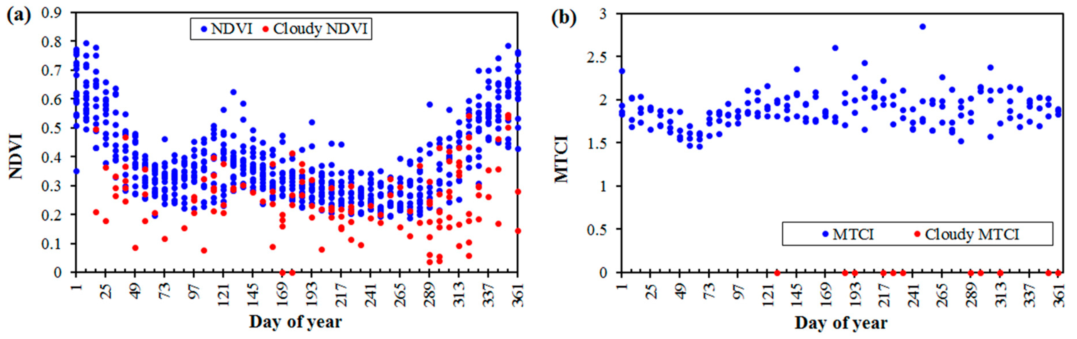
2.4. Quality Control

The quality of the extracted SOS in the Indian monsoon region is labeled by three criteria: the mean absolute fitting bias between the original NDVI and reconstructed NDVI (shortened to Bias), the roughness of the reconstructed vegetation growth trajectory (shortened to Roughness), and the data availability during the middle part of the vegetation growth period. The data availability is represented by the counts of valid observations between 15% and 85% of the VGA (shortened to Count70), and the count between 25% and 75% of VGA (shortened to Count50). If Bias > 0.07, Roughness > 0.06, or Count70 < 1, the QC was set as 1 (no data); else if Bias > 0.05, Roughness > 0.05, or Count50 < 1, the QC was set as 2 (poor quality); or else, if Bias ≤ 0.05, Roughness ≤ 0.05, and Count50 ≥ 1, the QC was set as 3 (good quality). The thresholds of Bias and Roughness used for QC = 1 were determined from the statistics of pixels (about 95%) across the entire study area. The pixel percentage was 95.41% for Bias ≤ 0.07, and the pixel percentage was 95.26% for Roughness ≤ 0.06.

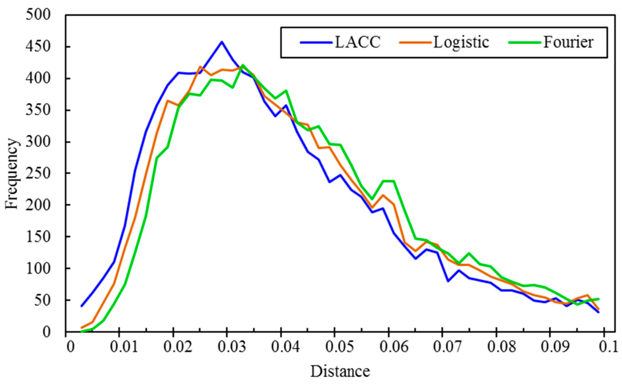
2.5. Comparison with Other Approaches for Modeling the Varied Vegetation Growth Trajectories

LACC was compared with Logistic and Fourier for modeling eight typical vegetation growth trajectories and extracting SOS. For the Logistic approach, the vegetation growth period was fitted by a logistic function:

$$\mathrm{NDVI}\left(\mathrm{t}\right)=\mathrm{MinNDVI}+\frac{\mathrm{MaxNDVI}-\mathrm{MinNDVI}}{1+\exp \left(\mathrm{ParaA}+\mathrm{ParaBt}\right)},$$

(2)

The t is the day of year (DOY), the NDVI(t) is the simulated NDVI value, and the ParaA and ParaB are the fitting parameters. The MaxNDVI and MinNDVI are the identified maximum and minimum NDVI. The maximum rate of change in curvature of the fitted logistic function (shortened to Zhang’s inflexion point) was used to determine SOS [13]. For the Fourier approach [16], four harmonics were used for the vegetation with one growing season, and six harmonics were used for croplands with double growing seasons. The SOS was identified using the first derivative value from negative to positive (curve valley point) [16].

To comprehensively evaluate the performance of LACC, Logistic, and Fourier for modeling the varied vegetation growth trajectories, 10,000 pixels were randomly selected at the locations with QC = 3 to create gaps in the reference NDVI to conduct an additional validation procedure. The reference NDVI was calculated as the average NDVI on the same day-of-year (DOY) across the complete time series (2000–2016) for each pixel location [34] using MODIS Collection 6 MOD09A1 data. The gaps were created by excluding the NDVI values following the temporal distributions of real clouds in 2006. After the reconstructions of the reference NDVI with gaps by the three approaches, the average distances between the reconstructed NDVI values and the excluded NDVI values in the reference NDVI were used to indicate the best approach.

2.6. Comparison of the Extracted SOS with Other Products

The GLOBMAP-IndianSOS product was compared with the MCD12Q2 phenology product (2001–2014) and the MERIS phenology product. The counts of valid SOS retrieval and the valid percentage between GLOBMAP-IndianSOS product and MCD12Q2 were compared. The counts of valid SOS retrieval during the 14 years (shortened to valid counts) were calculated for each pixel. The valid percentage of a product was calculated as the ratio of all valid counts to the total counts that should be retrieved. The comparison with the MERIS phenology product was used to evaluate the spatial patterns of the extracted SOS.

2.7. Evaluation of the Reliability of Retrieval Approach

Generally, in a small region, the meteorological conditions are nearly the same so that the effects of meteorological change on SOS should be similar. That is, if the land cover is unchanged, the advancement or postponement of SOS between two years should be synchronous in a small window. If the phenology retrieval is reliable, the change in SOS between two years for each pixel (SOSC) within a window should be approximately the same. The variability of SOSC within a window (5 × 5) was used to indicate the reliability of the LSP retrieval. The following steps were used to conduct the evaluation of variability for all retrievals: (1) the SOSC was calculated pixel by pixel; (2) the average SOSC was calculated for each window (5 × 5); and (3) the difference between pixel SOSC and window average SOSC (SOSC bias) was computed at each pixel within the window. The greater the SOSC bias was, the lower reliability of the LSP retrieval. The percentage of pixels with SOSC biases within ±10 days was used for quantitatively describing reliability.

For comparison, the same evaluation approach was used for deciduous broadleaf forests of North America and Europe (<55°N, cloud-free and snow-free) from the MCD12Q2 product, where data availability is sufficient and the SOS was demonstrated to be reliably extracted from satellite data [15,35,36]. So if the percentage of pixels for the extracted SOS with bias <±10 days is approximate to that of deciduous broadleaf forests in North America and Europe, the extracted SOS could be regarded as reliable.

3. Results

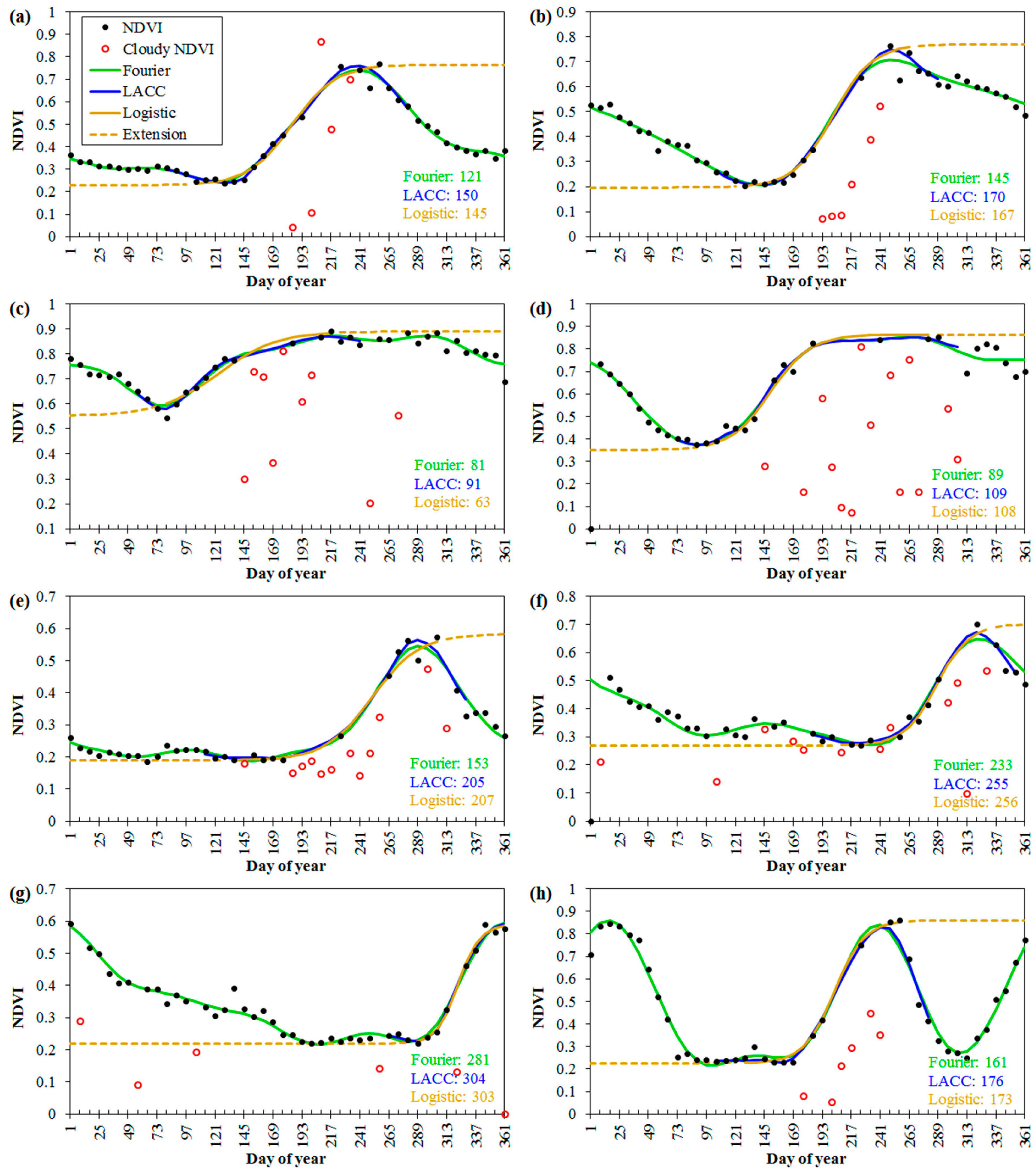
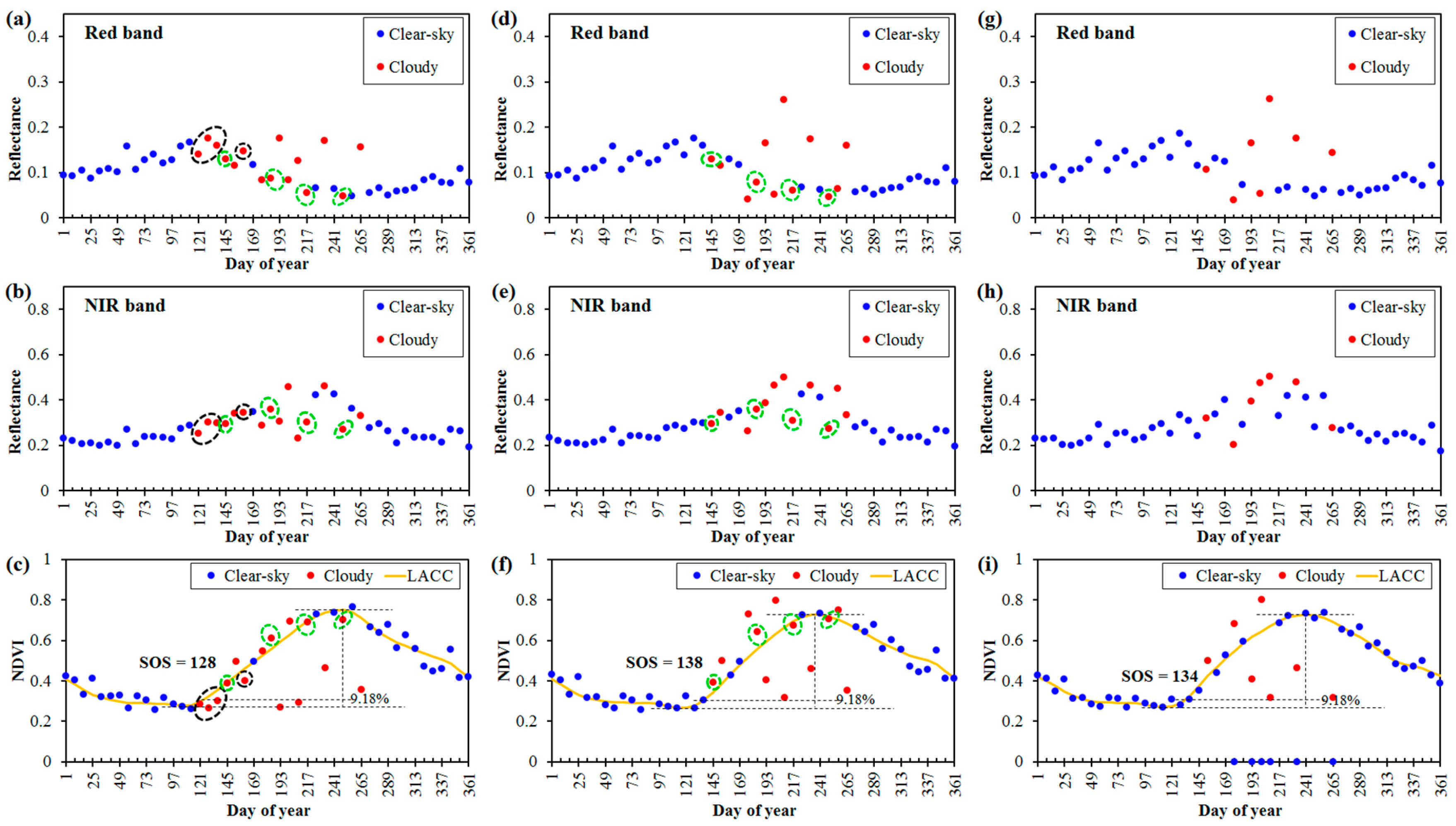
3.1. Modeling the Varied Vegetation Growth Trajectories

The vegetation growth trajectories in the Indian monsoon region vary from site to site. Several typical vegetation growth trajectories are shown in Figure 3: the vegetation grows quickly and withers quickly (Figure 3a), the vegetation grows quickly but withers slowly (Figure 3b), the vegetation growth has no dormancy stage (sharp curve valley in the trajectory) (Figure 3c), the vegetation growth has a long maturity stage (Figure 3d), the vegetation growth has a long dormancy stage and withers quickly (Figure 3e), the vegetation growth has a long dormancy stage but withers slowly (Figure 3f), the vegetation growth has a short dormancy stage and withers slowly (Figure 3g), and the double-cropping vegetation (Figure 3h).

Figure 3 also shows modeling of eight typical vegetation growth trajectories using the LACC approach, Fourier approach, and Logistic approach. Fourier performed well for the trajectories that had obvious curve valleys before vegetation growth. But for the trajectories with a long dormancy stage, spurious oscillations usually appeared for the Fourier, which would confuse the SOS identification by curve valley point. Uncertainties would exist if the wrong curve valley point was selected for identifying SOS; therefore, some measures should be taken to eliminate the influence of these spurious oscillations in Fourier. Logistic modeled the trajectories well during the vegetation growth period for most pixels, but it is inapplicable for trajectories with a sharp curve valley (Figure 3c), in which the extracted SOS with Zhang’s inflexion point [13] was smaller than the identified starting date of the vegetation growth period. This kind of situation commonly appeared in the eastern part (20°N–40°N, 89°E–90°E) and southern part (8°N–20°N, 74°E–84°E) of the Indian monsoon region. For the special vegetation growth trajectories, the piecewise logistic function approach should be modified by adding an impact factor [37,38], or using the adaptive local iterative logistic fitting method (ALILF) [18]. LACC solved the limitations associated with Logistic and Fourier for modeling trajectories with sharp curve valleys or a long dormancy stage, and the extracted SOS from LACC was very similar to that from Logistic, except for the trajectory with a sharp curve valley (Figure 3c) where Logistic was inapplicable. The extracted SOS from Fourier was noticeably smaller than that from Logistic and LACC, but for the trajectory with a sharp curve valley (Figure 3c) it was closer to the SOS from LACC than that from Logistic. Figure 4 presents the histograms of the distances between the reconstructed NDVI values by the three approaches and the excluded NDVI values in the time-series of reference NDVI. For the randomly selected 10,000 pixels, the average distances are 0.037 ± 0.0208 for LACC, 0.040 ± 0.0215 for Logistic, and 0.043 ± 0.0219 for Fourier. LACC had the smallest distances compared with Logistic and Fourier. These results indicated that LACC was more applicable for modeling the varied vegetation growth trajectories in the Indian monsoon region than Logistic and Fourier.

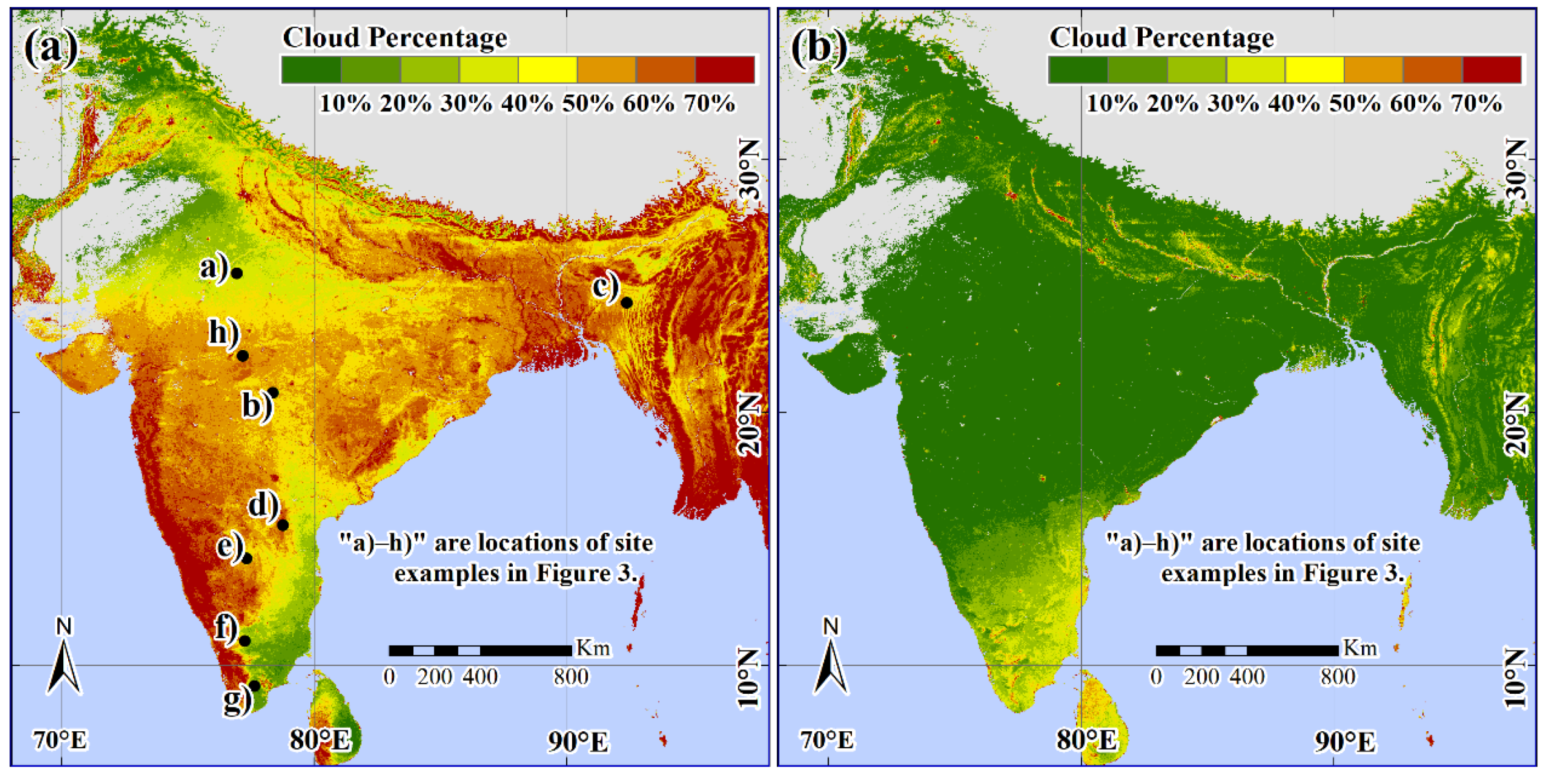
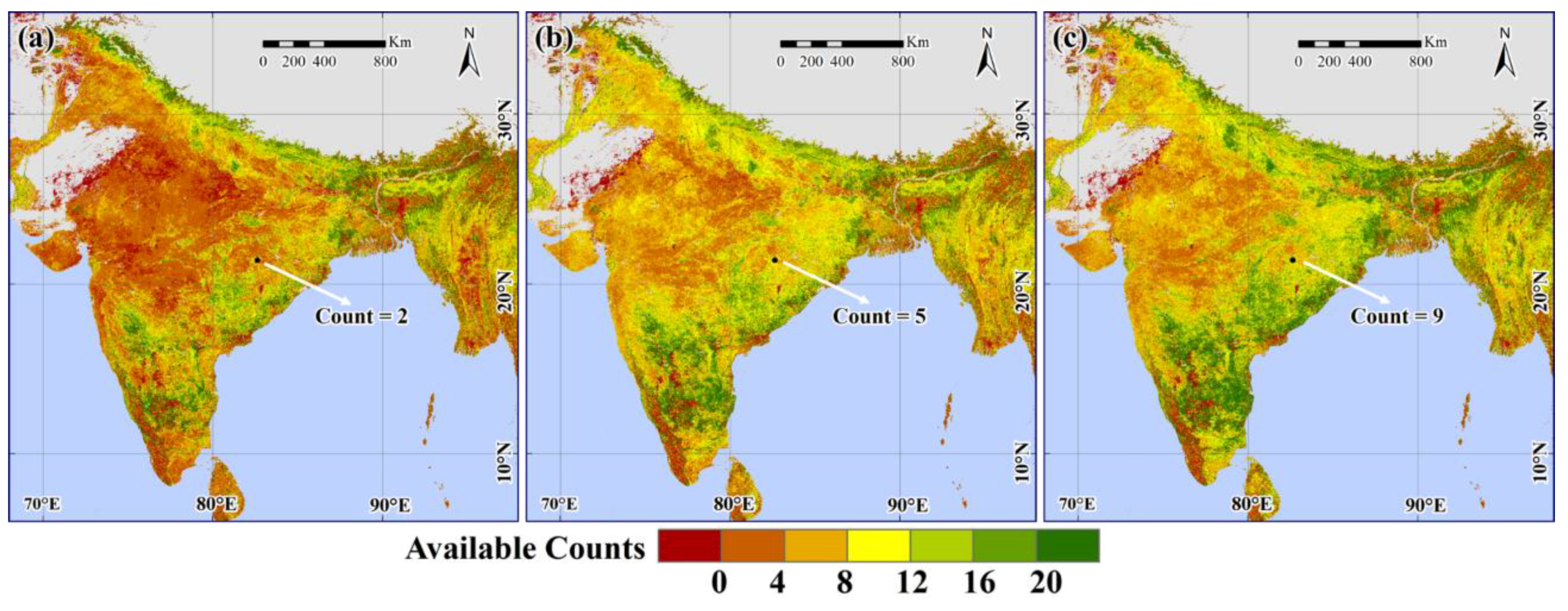
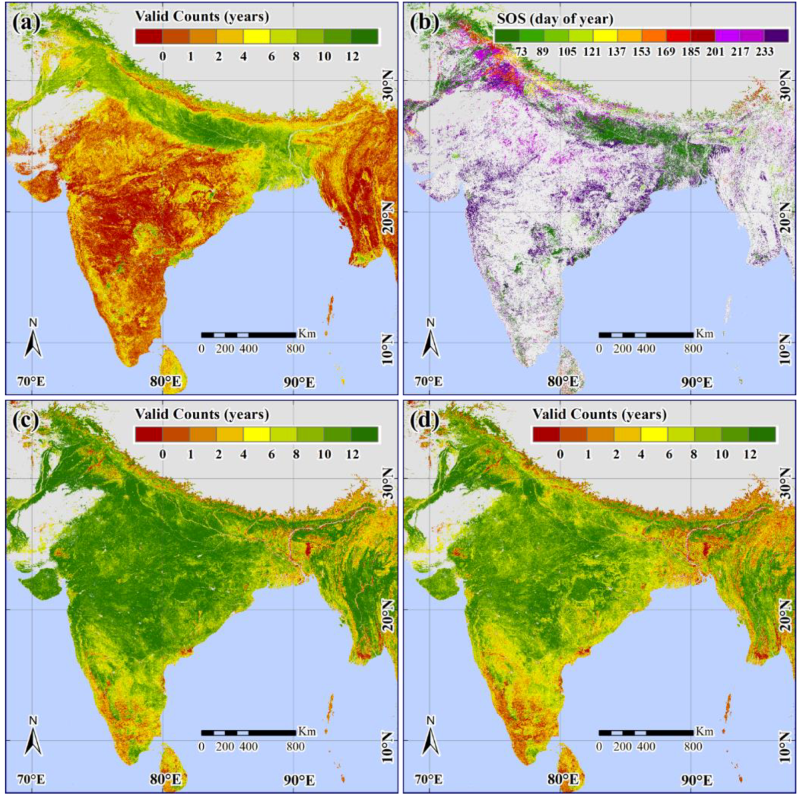
3.2. Statistics of Available Data in Rainy Season

Figure 5 shows the spatial distribution of available data counts during the 5% and 95% of VGA (Count90) from three data sources in 2006. These three data sources were all generated from MODIS surface reflectance data with different data processing procedures. Figure 5a is Collection 5 MOD09A1 screened by its cloud mask (hereafter referred to as MOD09A1_C5); Figure 5b is Collection 6 MOD09A1 screened by its cloud mask (hereafter referred to as MOD09A1_C6); and Figure 5c is Collection 6 MOD09A1 screened by IBCD cloud detection approach (hereafter referred to as IBCD_C6). The pixels with VGA < 0.2 were excluded from the statistical analyses.

Table 1. Statistics for available data counts during the 5% and 95% of VGA (Count90) from three data sources in 2006.

Level of Statistics	MOD09A1_C5	MOD09A1_C6	IBCD_C6
Count90 ≥ 5	55.42%	76.47%	79.59%
Count90 ≥ 8	39.62%	55.96%	60.24%

presents the statistics of Count90 from three data sources at two levels: Count90 ≥ 5 (the basic requirement for SOS retrieval) and Count90 ≥ 8 (a higher criterion for SOS retrieval). IBCD_C6 had the highest data availability for both levels. The data availability of MOD09A1_C6 was higher than MOD09A1_C5, supporting the improvement of the MODIS Collection 6 cloud mask. However, there were still some overestimations (clear-sky observations labelled as clouds) in the MODIS Collection 6 cloud mask. Figure 6 shows a temporal example of the data availability for the three data sources. There were eight clear-sky observations labeled as clouds in MOD09A1_C5, in which four could be identified by both the MODIS Collection 6 cloud mask and the IBCD approach, and the remaining four could only be identified by the IBCD approach. The extracted SOS from MOD09A1_C5 was the smallest (DOY 128), and the largest (DOY 138) was from MOD09A1_C6. The advanced SOS of MOD09A1_C5 may have resulted from the loss of three key observations around the curve valley, while the delayed SOS of MOD09A1_C6 was influenced by both the BRDF correction and the loss of three observations during the vegetation growth period.

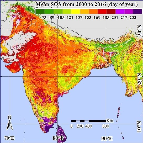
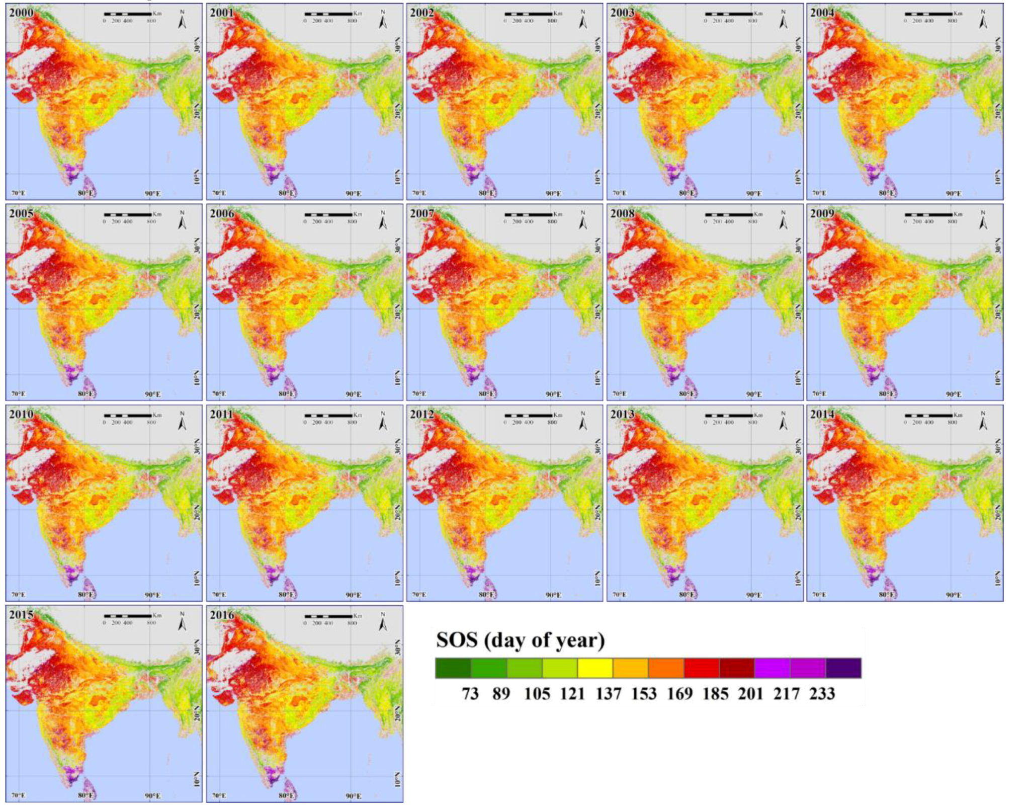
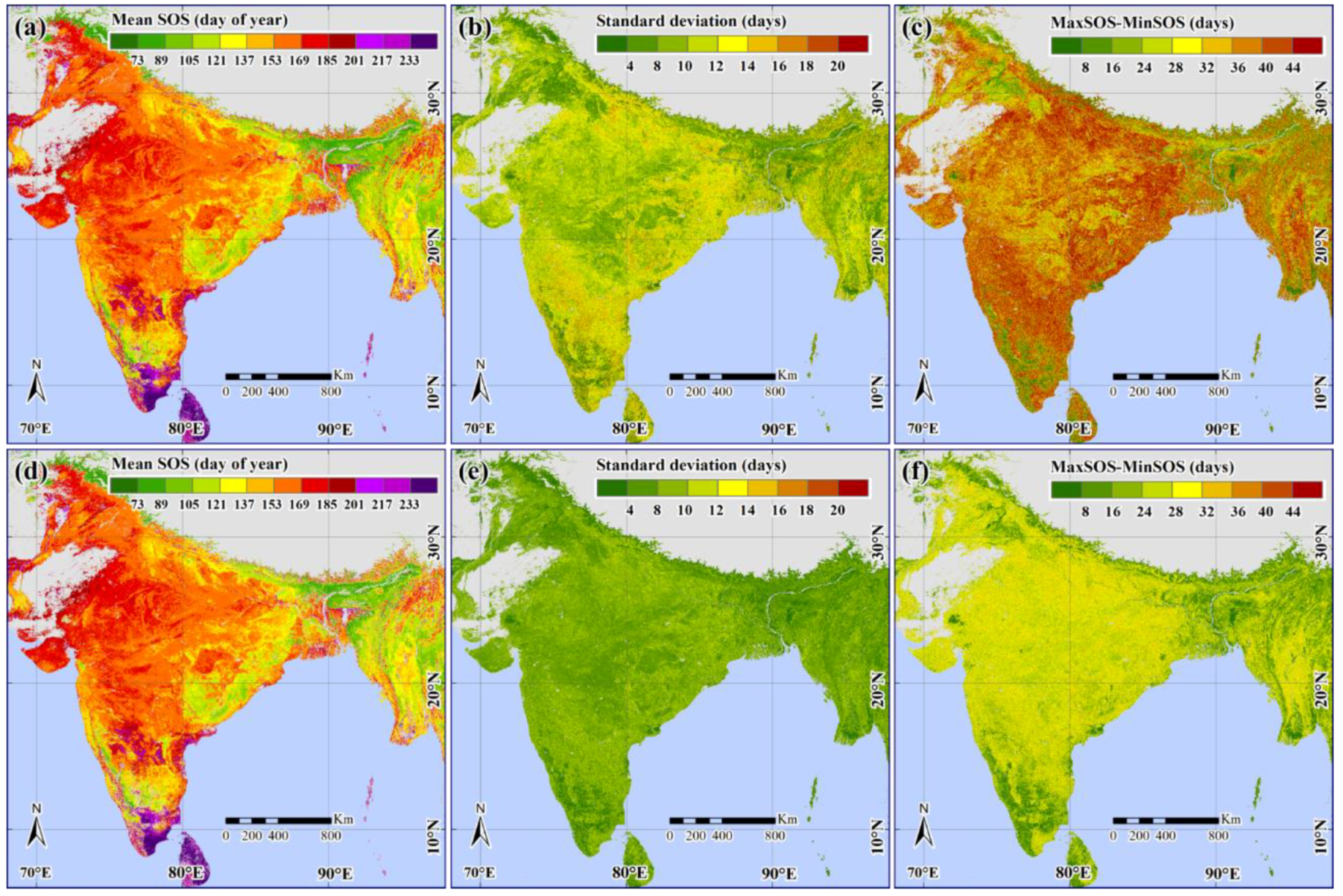
3.3. Results of the Extracted SOS in the India Monsoon Region

Figure 7 shows the extracted SOS (QC > 1) for the Indian monsoon region from 2000 to 2016. Their mean value, standard deviation, and difference between the maximum and minimum value are presented in Figure 8. The spatial patterns were obvious. A gradual appearance of SOS appeared from the southwest (<DOY 105) toward the central part of India (>DOY 169), from the southeast (<DOY 121) toward the northwest part of India (>DOY 169), and from the east (<DOY 105) toward the western part of India (>DOY 169). These patterns are coincident with the migration directions of the southwest monsoon. The eastern part of India and India’s western coast had the smallest SOS (<DOY 105). The southern parts of India, such as Tamil Nadu and Kerala, exhibited the largest SOS (>DOY 233), where the vegetation growth cycle mainly began in September, matured in December, and withered in January of the following year. This late growing season could also be indicated by the date of the Tamil Hindu harvest festival in the Indian state of Tamil Nadu (celebrated in the middle of January). The standard deviation of SOS from the different years mainly ranged from 1 day to 16 days (Figure 8b), and the difference between the maximum and minimum SOS mainly ranged from 8 days to 40 days (Figure 8c). When excluding SOS with poor quality (QC = 2), the mean SOS showed no significant changes, but the standard deviation and the difference between the maximum and minimum SOS became much smaller.

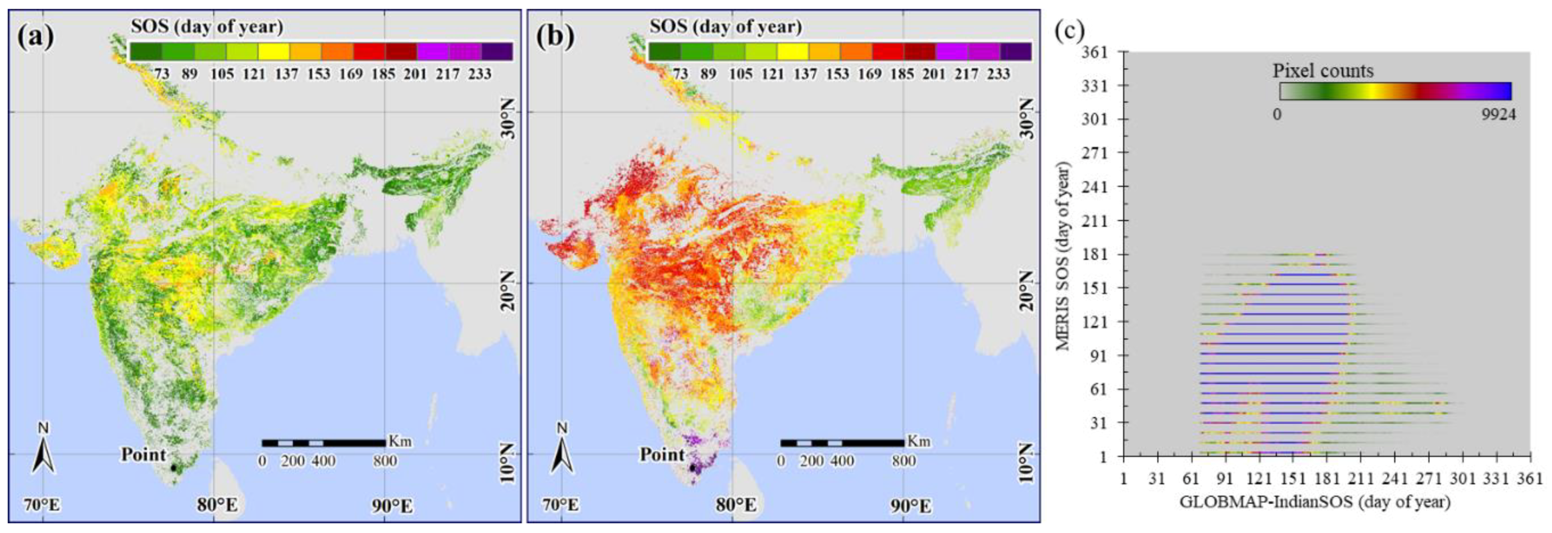
3.4. Comparison with the MERIS Phenology Product

The GLOBMAP-IndianSOS product (QC > 1) was compared with the MERIS phenology product [16]. Figure 9a shows the SOS from the MERIS phenology product in 2006 where the double-cropping lands were excluded. Figure 9b presents the SOS from the GLOBMAP-IndianSOS product in 2006. Figure 9c shows the density scatterplot of these two products. Compared with the MERIS phenology product, the SOS for a vast majority of pixels in the GLOBMAP-IndianSOS product was delayed, and an early SOS appeared in the eastern and southeastern parts of India. The scale effects between 500 m and 4.6 km, as well as different determinations of SOS and different representations of vegetation growth cycles by NDVI and MTCI, likely explain these differences. First, the SOS at a coarse resolution was possible to simulate by selecting the date at the 30th percentile SOS at finer resolution [39], resulting in the advanced SOS at a coarse resolution. Second, the SOS in the MERIS phenology product was identified using the first derivative value from negative to positive (valley point), whereas the SOS in the GLOBMAP-IndianSOS product was determined from the date when NDVI exceeded 9.18% of VGA. The valley point in the Fourier-based approach was equal to 0% of VGA, which was certainly earlier than that from 9.18% of VGA. These two reasons can explain most of the delayed SOS (30 days for most pixels) in the GLOBMAP-IndianSOS product. The most obvious difference appeared in the southern part of India, such as in some parts of Tamil Nadu and Kerala, where the GLOBMAP-IndianSOS product exhibited the latest SOS (>DOY 244) and the SOS from the MERIS phenology product was early (<DOY 65). The early SOS in these regions was explained with no clear phenology pattern of MTCI [16], since other approaches such as the Whittaker smoother, asymmetric Gaussian function, and double logistic function also extract early SOS from MTCI [17]. As shown in Figure 10, the MTCI is unable to clearly describe the cropping season from September to January for these pixels, but it is described by the NDVI. The late SOS in Tamil Nadu (11.77°N, 78.20°E) was also extracted by Prasad, Badarinath, and Eaturu [6] from the average AVHRR-NDVI from 1990 to 2000, which supports the results of the GLOBMAP-IndianSOS product.

The GLOBMAP-IndianSOS product was also compared with the phenology results that were derived from MOD13C1 NDVI and EVI (5.6 km, 16 day) [19]. For the natural vegetation located in the central parts of the Indian monsoon region (14°N–26°N, 70°E–88°E), the extracted SOS in the GLOBMAP-IndianSOS product varied from the DOY of 120 to 180, which corresponded with SOS derived from the average MODIS-NDVI and the average MODIS-EVI from 2001 to 2010 as shown in Figure 3b,c in the study of Jeganathan and Nishant [19].

3.5. Comparison with the MCD12Q2 Product

Figure 11a shows the counts of valid SOS retrievals in the MCD12Q2 product from 2001 to 2014. Except for the double-cropping areas, the counts of valid SOS retrieval for almost all pixels were less than 4 in the MCD12Q2 product in the Indian monsoon region. The valid percentage of SOS in the MCD12Q2 product from 2001 to 2014 was 29.30%. Figure 11b shows the spatial distribution of SOS for the MCD12Q2 product in 2006. The SOS for most of the pixels with one growing season ranged from DOY 201 to DOY 265. For the croplands with double or triple growing seasons in the Himalaya region, obvious differences of SOS were observed between the GLOBMAP-IndianSOS product and the MCD12Q2 product. Large differences in SOS could be mainly explained by different growing seasons used to extract SOS, and small differences might be explained by different representations of vegetation growth cycles by NDVI and EVI. Figure 11c,d show the counts of valid SOS retrievals from the GLOBMAP-IndianSOS product from 2001 to 2014 with QC > 1 and QC > 2, respectively. The statistics of pixels with different counts of valid SOS retrievals in the GLOBMAP-IndianSOS product and the statistics of pixels with different improved counts of valid SOS retrievals compared with MCD12Q2 product from 2001 to 2014 are listed in

Table 2. The percentages of pixels with different counts of valid SOS retrievals in the GLOBMAP-IndianSOS product from 2001 to 2014.

Level of Statistics	% (QC > 1)	% (QC > 2)
Valid counts = 14	16.98%	6.53%
Valid counts ≥ 12	46.59%	27.12%
Valid counts ≥ 10	63.72%	46.75%
Valid counts ≥ 8	73.93%	61.63%
Valid counts ≥ 6	81.24%	72.66%
Valid counts ≥ 4	88.07%	81.87%
Valid counts ≥ 1	97.78%	96.02%

and

Table 3. The percentages of pixels with different improved counts of valid SOS retrievals compared with the MCD12Q2 product from 2001 to 2014.

Level of Statistics	% (QC > 1)	% (QC > 2)
Improved counts = 14	2.91%	0.97%
Improved counts ≥ 12	15.59%	7.57%
Improved counts ≥ 10	30.98%	19.30%
Improved counts ≥ 8	44.70%	32.74%
Improved counts ≥ 6	56.33%	45.57%
Improved counts ≥ 4	66.99%	57.54%
Improved counts ≥ 1	81.10%	79.05%

, respectively. Exactly 16.98% of pixels had a valid SOS retrieval for all years in the GLOBMAP-IndianSOS product, and compared with the MCD12Q2 product, 2.91% of pixels improved from no valid SOS retrieval to all valid SOS retrieval during the 14 years; such pixels were mainly located in the central and eastern parts of the study area. The valid percentage of SOS in the GLOBMAP-IndianSOS product from 2001 to 2014 was 69.76%, which improved by 40.46% compared with the MCD12Q2 product. When excluding SOS with poor quality, the improvement was 29.56%.

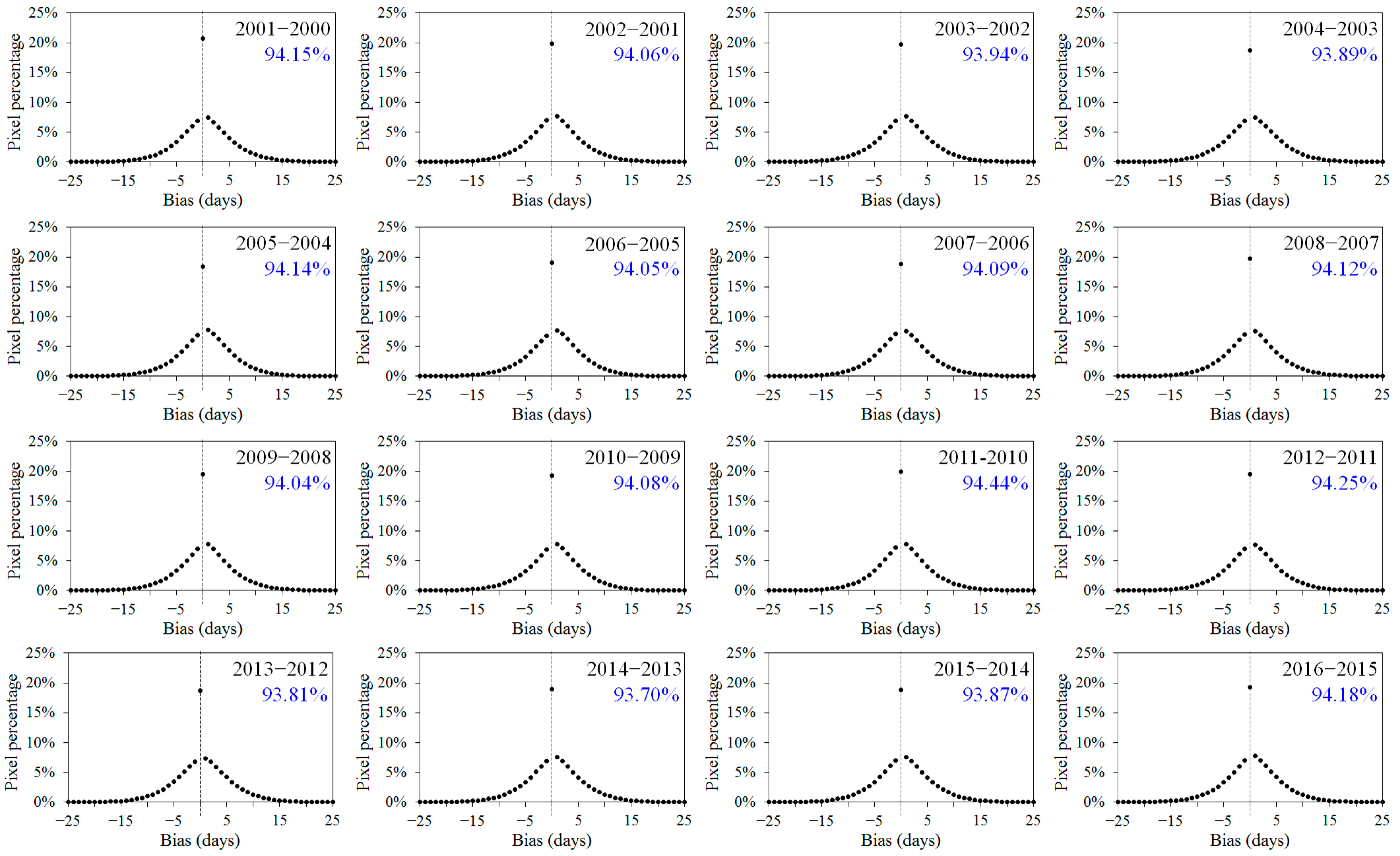
3.6. The Reliability of the Retrieval Approach

Figure 12 shows bias histograms of SOS differences compared with the average value in each local widow (5 × 5) from 2000 to 2016. The pixel percentages with biases within ±10 days for the continuous two years were approximately 94%, which were very close to the pixel percentages for deciduous broadleaf forests in North America and Europe (94.24%) from the MCD12Q2 product between 2005 and 2006. The highest pixel percentage appeared between 2010 and 2011, and the lowest pixel percentage occurred between 2013 and 2014. For the SOS with lower quality, the evaluation of reliability was also conducted for two continuous years between 2013 and 2014. The pixel percentage for the biases within ±10 days was 78.48% for SOS with QC > 1, indicating the lower reliability of the extracted SOS with poor quality. These results demonstrated that the reliability of the extracted SOS with QC > 2 in the Indian monsoon region was very similar to that of deciduous broadleaf forests in North America and Europe.

4. Conclusions

This study modified the extraction of the start of the growing season in the Indian monsoon region by modeling the varied vegetation growth trajectories and accurately identifying available data for the rainy season. The GLOBMAP-IndianSOS product was generated from Collection 6 MOD09A1 at 500 m resolution from 2000 to 2016. The SOS showed similar spatial patterns with other products, and the gradual transition of the SOS was coincident with the migration directions of the southwest monsoon. Compared with the Collection 5 MCD12Q2 phenology product, the valid percentage of SOS in the GLOBMAP-IndianSOS product improved by 40.46%, and its reliability was demonstrated to be similar to that of deciduous broadleaf forest in North America and Europe. This product could serve as a basis for understanding changes in the Indian monsoon and its influence on terrestrial ecosystem productivity in Indian monsoon region, ultimately helping to predict future climate change.

References

1. Fu, Y.S.H.; Zhao, H.F.; Piao, S.L.; Peaucelle, M.; Peng, S.S.; Zhou, G.Y.; Ciais, P.; Huang, M.T.; Menzel, A.; Uelas, J.P.; et al. Declining global warming effects on the phenology of spring leaf unfolding. Nature 2015, 526, 104–107. [Google Scholar] [CrossRef] [PubMed]
2. Ge, Q.S.; Wang, H.J.; Rutishauser, T.; Dai, J.H. Phenological response to climate change in China: A meta-analysis. Glob. Chang. Biol. 2015, 21, 265–274. [Google Scholar] [CrossRef] [PubMed]
3. Wu, J.; Albert, L.P.; Lopes, A.P.; Restrepo-Coupe, N.; Hayek, M.; Wiedemann, K.T.; Guan, K.Y.; Stark, S.C.; Christoffersen, B.; Prohaska, N.; et al. Leaf development and demography explain photosynthetic seasonality in Amazon evergreen forests. Science 2016, 351, 972–976. [Google Scholar] [CrossRef] [PubMed]
4. Zhou, L.; Tian, Y.; Myneni, R.B.; Ciais, P.; Saatchi, S.; Liu, Y.Y.; Piao, S.; Chen, H.; Vermote, E.F.; Song, C.; et al. Widespread decline of Congo rainforest greenness in the past decade. Nature 2014, 509, 86–90. [Google Scholar] [CrossRef] [PubMed]
5. Fu, Y.H.; Piao, S.; Zhao, H.; Jeong, S.-J.; Wang, X.; Vitasse, Y.; Ciais, P.; Janssens, I.A. Unexpected role of winter precipitation in determining heat requirement for spring vegetation green-up at northern middle and high latitudes. Glob. Chang. Biol. 2014, 20, 3743–3755. [Google Scholar] [CrossRef] [PubMed]
6. Prasad, V.K.; Badarinath, K.V.S.; Eaturu, A. Spatial patterns of vegetation phenology metrics and related climatic controls of eight contrasting forest types in India—Analysis from remote sensing datasets. Theor. Appl. Climatol. 2007, 89, 95–107. [Google Scholar] [CrossRef]
7. Singh, D.; Tsiang, M.; Rajaratnam, B.; Diffenbaugh, N.S. Observed changes in extreme wet and dry spells during the South Asian summer monsoon season. Nat. Clim. Chang. 2014, 4, 456–461. [Google Scholar] [CrossRef]
8. Vinnarasi, R.; Dhanya, C.T. Changing characteristics of extreme wet and dry spells of Indian monsoon rainfall. J. Geophys. Res. Atmos. 2016, 121, 2146–2160. [Google Scholar] [CrossRef]
9. Ramarao, M.V.S.; Krishnan, R.; Sanjay, J.; Sabin, T.P. Understanding land surface response to changing South Asian monsoon in a warming climate. Earth Syst. Dyn. 2015, 6, 569–582. [Google Scholar] [CrossRef]
10. Karmakar, N.; Chakraborty, A.; Nanjundiah, R.S. Decreasing intensity of monsoon low-frequency intraseasonal variability over India. Environ. Res. Lett. 2015, 10. [Google Scholar] [CrossRef]
11. Chakraborty, A.; Seshasai, M.V.R.; Dadhwal, V.K. Geo-spatial analysis of the temporal trends of kharif crop phenology metrics over India and its relationships with rainfall parameters. Environ. Monit. Assess. 2014, 186, 4531–4542. [Google Scholar] [CrossRef] [PubMed]
12. Liu, R.G.; Liu, Y. Generation of new cloud masks from MODIS land surface reflectance products. Remote Sens. Environ. 2013, 133, 21–37. [Google Scholar] [CrossRef]
13. Zhang, X.Y.; Friedl, M.A.; Schaaf, C.B.; Strahler, A.H.; Hodges, J.C.F.; Gao, F.; Reed, B.C.; Huete, A. Monitoring vegetation phenology using MODIS. Remote Sens. Environ. 2003, 84, 471–475. [Google Scholar] [CrossRef]
14. Zhang, X.Y.; Friedl, M.A.; Schaaf, C.B. Global vegetation phenology from moderate resolution imaging spectroradiometer (MODIS): Evaluation of global patterns and comparison with in situ measurements. J. Geophys. Res.-Biogeosci. 2006, 111. [Google Scholar] [CrossRef]
15. Ganguly, S.; Friedl, M.A.; Tan, B.; Zhang, X.; Verma, M. Land surface phenology from MODIS: Characterization of the Collection 5 global land cover dynamics product. Remote Sens. Environ. 2010, 114, 1805–1816. [Google Scholar] [CrossRef]
16. Dash, J.; Jeganathan, C.; Atkinson, P.M. The use of MERIS terrestrial chlorophyll index to study spatio-temporal variation in vegetation phenology over India. Remote Sens. Environ. 2010, 114, 1388–1402. [Google Scholar] [CrossRef]
17. Atkinson, P.M.; Jeganathan, C.; Dash, J.; Atzberger, C. Inter-comparison of four models for smoothing satellite sensor time-series data to estimate vegetation phenology. Remote Sens. Environ. 2012, 123, 400–417. [Google Scholar] [CrossRef]
18. Cao, R.Y.; Chen, J.; Shen, M.G.; Tang, Y.H. An improved logistic method for detecting spring vegetation phenology in grasslands from MODIS EVI time-series data. Agric. For. Meteorol. 2015, 200, 9–20. [Google Scholar] [CrossRef]
19. Jeganathan, C.; Nishant, N. Scrutinising MODIS and GIMMS vegetation indices for extracting growth rhythm of natural vegetation in India. J. Indian Soc. Remote Sens. 2014, 42, 397–408. [Google Scholar] [CrossRef]
20. Duncan, J.M.A.; Dash, J.; Atkinson, P.M. Spatio-temporal dynamics in the phenology of croplands across the Indo-Gangetic Plains. Adv. Space Res. 2014, 54, 710–725. [Google Scholar] [CrossRef]
21. Verger, A.; Baret, F.; Weiss, M.; Kandasamy, S.; Vermote, E. The CACAO method for smoothing, gap filling, and characterizing seasonal anomalies in satellite time series. IEEE Trans. Geosci. Remote Sens. 2013, 51, 1963–1972. [Google Scholar] [CrossRef]
22. Kandasamy, S.; Baret, F.; Verger, A.; Neveux, P.; Weiss, M. A comparison of methods for smoothing and gap filling time series of remote sensing observations—Application to MODIS LAI products. Biogeosciences 2013, 10, 4055–4071. [Google Scholar] [CrossRef]
23. Liu, R.; Shang, R.; Liu, Y.; Lu, X. Global evaluation of gap-filling approaches for seasonal NDVI with considering vegetation growth trajectory, protection of key point, noise resistance and curve stability. Remote Sens. Environ. 2017, 189, 164–179. [Google Scholar] [CrossRef]
24. Lucht, W.; Schaaf, C.B.; Strahler, A.H. An algorithm for the retrieval of albedo from space using semiempirical BRDF models. IEEE Trans. Geosci. Remote Sens. 2000, 38, 977–998. [Google Scholar] [CrossRef]
25. Peng, S.; Piao, S.; Ciais, P.; Myneni, R.B.; Chen, A.; Chevallier, F.; Dolman, A.J.; Janssens, I.A.; Penuelas, J.; Zhang, G.; et al. Asymmetric effects of daytime and night-time warming on Northern Hemisphere vegetation. Nature 2013, 501, 88–92. [Google Scholar] [CrossRef] [PubMed]
26. Piao, S.; Tan, J.; Chen, A.; Fu, Y.H.; Ciais, P.; Liu, Q.; Janssens, I.A.; Vicca, S.; Zeng, Z.; Jeong, S.-J.; et al. Leaf onset in the northern hemisphere triggered by daytime temperature. Nat. Commun. 2015, 6, 6911. [Google Scholar] [CrossRef] [PubMed]
27. Balzarolo, M.; Vicca, S.; Nguy-Robertson, A.L.; Bonal, D.; Elbers, J.A.; Fu, Y.H.; Grunwald, T.; Horemans, J.A.; Papale, D.; Penuelas, J.; et al. Matching the phenology of net ecosystem exchange and vegetation indices estimated with MODIS and FLUXNET in-situ observations. Remote Sens. Environ. 2016, 174, 290–300. [Google Scholar] [CrossRef]
28. Vermote, E.F.; Kotchenova, S. Atmospheric correction for the monitoring of land surfaces. J. Geophys. Res.-Atmos. 2008, 113. [Google Scholar] [CrossRef]
29. Malik, N.; Bookhagen, B.; Mucha, P.J. Spatiotemporal patterns and trends of Indian monsoonal rainfall extremes. Geophys. Res. Lett. 2016, 43, 1710–1717. [Google Scholar] [CrossRef] [PubMed]
30. Bicheron, P.; Defourny, P.; Brockmann, C.; Schouten, L.; Vancutsem, C.; Huc, M.; Bontemps, S.; Leroy, M.; Achard, F.; Herold, M. Globcover: Products description and validation report. Foro Mundial De La Salud 2011, 17, 285–287. [Google Scholar]
31. Chen, J.M.; Deng, F.; Chen, M. Locally adjusted cubic-spline capping for reconstructing seasonal trajectories of a satellite-derived surface parameter. IEEE Trans. Geosci. Remote Sens. 2006, 44, 2230–2238. [Google Scholar] [CrossRef]
32. He, L.M.; Liu, J.; Chen, J.M.; Croft, H.; Wang, R.; Sprintsin, M.; Zheng, T.R.; Ryu, Y.; Piseke, J.; Gonsamo, A.; et al. Inter- and intra-annual variations of clumping index derived from the MODIS BRDF product. Int. J. Appl. Earth Obs. Geoinf. 2016, 44, 53–60. [Google Scholar] [CrossRef]
33. Liu, R. Compositing the minimum NDVI for MODIS data. IEEE Trans. Geosci. Remote Sens. 2017, 55, 1396–1406. [Google Scholar] [CrossRef]
34. Shang, R.; Liu, R.; Xu, M.; Liu, Y.; Zuo, L.; Ge, Q. The relationship between the threshold-based and the inflexion-based approaches in extraction of land surface phenology. Remote Sens. Environ. 2017, 199, 167–170. [Google Scholar] [CrossRef]
35. Nijland, W.; Bolton, D.K.; Coops, N.C.; Stenhouse, G. Imaging phenology; scaling from camera plots to landscapes. Remote Sens. Environ. 2016, 177, 13–20. [Google Scholar] [CrossRef]
36. Rodriguez-Galiano, V.F.; Dash, J.; Atkinson, P.M. Intercomparison of satellite sensor land surface phenology and ground phenology in Europe. Geophys. Res. Lett. 2015, 42, 2253–2260. [Google Scholar] [CrossRef] [Green Version]
37. Zhang, X.Y. Reconstruction of a complete global time series of daily vegetation index trajectory from long-term AVHRR data. Remote Sens. Environ. 2015, 156, 457–472. [Google Scholar] [CrossRef]
38. Elmore, A.J.; Guinn, S.M.; Minsley, B.J.; Richardson, A.D. Landscape controls on the timing of spring, autumn, and growing season length in mid-Atlantic forests. Glob. Chang. Biol. 2012, 18, 656–674. [Google Scholar] [CrossRef]
39. Zhang, X.Y.; Wang, J.M.; Gao, F.; Liu, Y.; Schaaf, C.; Friedl, M.; Yu, Y.Y.; Jayavelu, S.; Gray, J.; Liu, L.L.; et al. Exploration of scaling effects on coarse resolution land surface phenology. Remote Sens. Environ. 2017, 190, 318–330. [Google Scholar] [CrossRef]
Figure 1. The vegetation map of the study area derived from the Globcover2009 dataset.
Remotesensing 10 00122 g001
Figure 2. The percentage of cloud cover from 2000 to 2016 during the southwest monsoon season (June to September) (a) and the post-monsoon season (October to November); (b) in MOD09A1. The black points are the locations of the eight examples shown in Figure 3.
Remotesensing 10 00122 g002
Figure 3. Typical vegetation growth trajectories fitted by the Fourier approach, and locally fitted by the Logistic approach and the LACC approach in 2006 (Locations are labelled in Figure 2a): (a) rain-fed croplands, (b) croplands/vegetation mosaic, (c) closed to open shrubland, (d) closed broadleaved deciduous forest, (e) croplands/vegetation mosaic, (f) croplands/vegetation mosaic, (g) irrigated croplands, and (h) irrigated croplands. All the symbols are explained in Figure 3a. The extracted SOS from the Fourier, LACC, and Logistic approach are labelled in the lower-right corner.
Remotesensing 10 00122 g003
Figure 4. Histogram of distances between the reconstructed NDVI values from LACC, Logistic, and Fourier approaches, and the excluded NDVI values in the time-series of reference NDVI.
Remotesensing 10 00122 g004
Figure 5. The spatial distribution of Count90 for three different data sources in 2006: (a) MOD09A1_C5, (b) MOD09A1_C6, and (c) IBCD_C6. The black point indicates the location of Figure 6.
Remotesensing 10 00122 g005
Figure 6. A temporal example (82.51°E, 21.49°N) in 2006 that illustrates the data availability and the extracted SOS for three different data sources. (ac) are red band and NIR band reflectance in MOD09A1_C5 and their calculated NDVI, (df) are red band and NIR band reflectance in MOD09A1_C6 and their calculated NDVI, and (gi) are cloud-screened and BRDF-corrected red band and NIR band reflectance and their calculated NDVI. The red points in the black ellipses are clear-sky observations that were labeled as clouds in MOD09A1_C5. The red points in the green ellipses are clear-sky observations labeled as clouds in MOD09A1_C5 and MOD09A1_C6.
Remotesensing 10 00122 g006
Figure 7. The SOS in the Indian monsoon region from 2000 to 2016.
Remotesensing 10 00122 g007
Figure 8. The mean SOS (a,d), standard deviation (b,e), and difference between the maximum and minimum SOS (e,f) in the Indian monsoon region from 2000 to 2016. (ac) are calculated from SOS with QC > 1, and (df) are calculated from SOS with QC > 2.
Remotesensing 10 00122 g008
Figure 9. (a) The SOS derived from MERIS Terrestrial Chlorophyll Index data in 2006 (the croplands with more than one growing season were masked), (b) the SOS from the GLOBMAP-IndianSOS product in 2006, and (c) the density scatterplot of these two products.
Remotesensing 10 00122 g009
Figure 10. Typical example of different vegetation growth trajectory represented by NDVI from 2000 to 2016 (a) and represented by MTCI from 2003 to 2006 (b) in the southern part of India (9.052°N, 77.496°E).
Remotesensing 10 00122 g010
Figure 11. (a) The counts of valid SOS retrievals in the MOD12Q2 product from 2001 to 2014, (b) the SOS in the MOD12Q2 product in 2006, (c) the counts of valid SOS retrievals in the GLOBMAP-IndianSOS product with QC > 1 from 2001 to 2014, (d) the counts of valid SOS retrievals in the GLOBMAP-IndianSOS product with QC > 2 from 2001 to 2014.
Remotesensing 10 00122 g011
Figure 12. The bias histograms of SOS differences compared with the average value in each local widow (5 × 5). The percentage listed in the blue color is for the statistics of biases within ±10 days.
Remotesensing 10 00122 g012