1. Introduction
The boreal zone land cover has a very significant influence on the northern hemisphere albedo and is an important component of the northern hemisphere carbon budget [
1,
2]. The boreal forest zone is sensitive to changes in local and global climate [
3]. Forest transition zones react to changes in mean temperature and moisture conditions in the long term [
4] whereas changes in, for example, forest leaf area index (LAI) through defoliation indicate stress factors in shorter time scale [
5]. Also the timing of the phenological phase transitions is an important indicator of global climatological processes [
6].
LAI is one of the Essential Climate Variables (ECV) defined in the Implementation Plan for the Global Observing System for Climate in Support of the United Nations Framework Convention on Climate Change
(UNFCCC) [
7]. Leaf Area Index (LAI) quantifies the amount of leaf material in an ecosystem, and is a measure of the potential of the vegetation of photosynthesis, respiration, rain interception, and other processes that link vegetation to climate. Consequently, LAI appears as a key variable in many models describing vegetation-atmosphere interactions, particularly with respect to the carbon and water cycles [
8]. For vegetated land cover, semi-empirical relationships between the surface albedo and LAI are used [
9]. The interest in information on LAI distribution and changes has grown substantially in recent decades, due to its importance for climate models and the developing capability for LAI estimation over large areas using satellite measurements. The development and validation of satellite based LAI estimation methods require reliable
in situ measurements of LAI. For large areas of tall vegetation it is difficult to get aerially representative ground truth using direct or indirect methods [
10,
11], especially in regions of difficult accessibility.
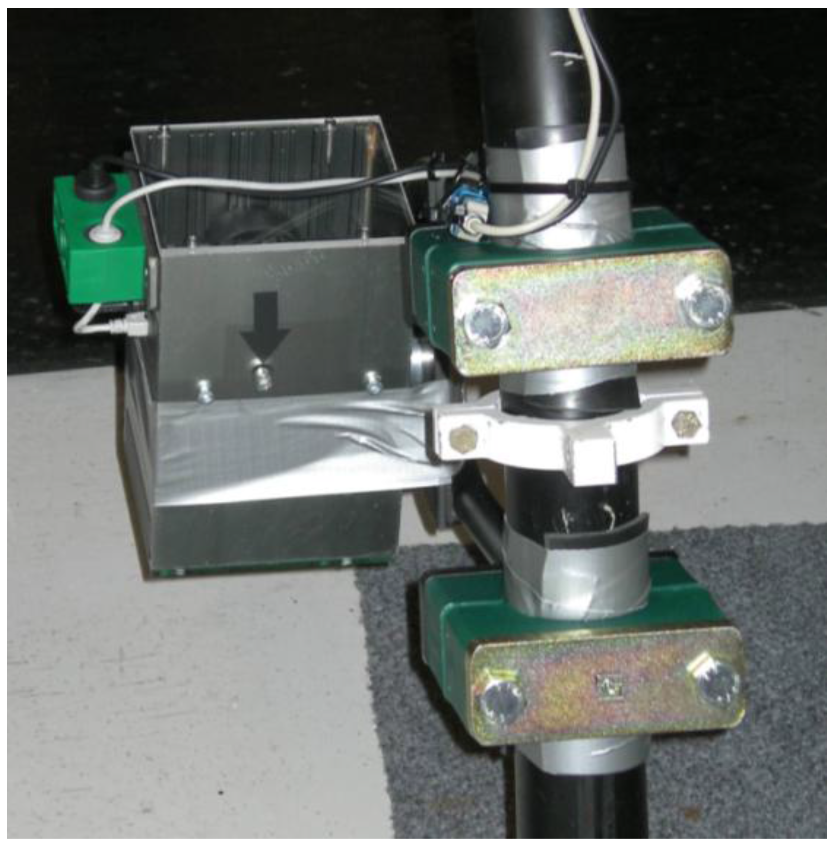
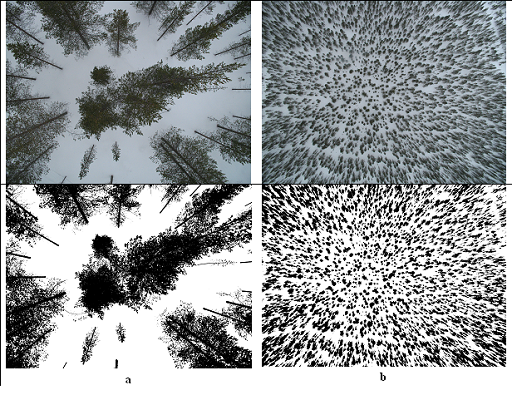
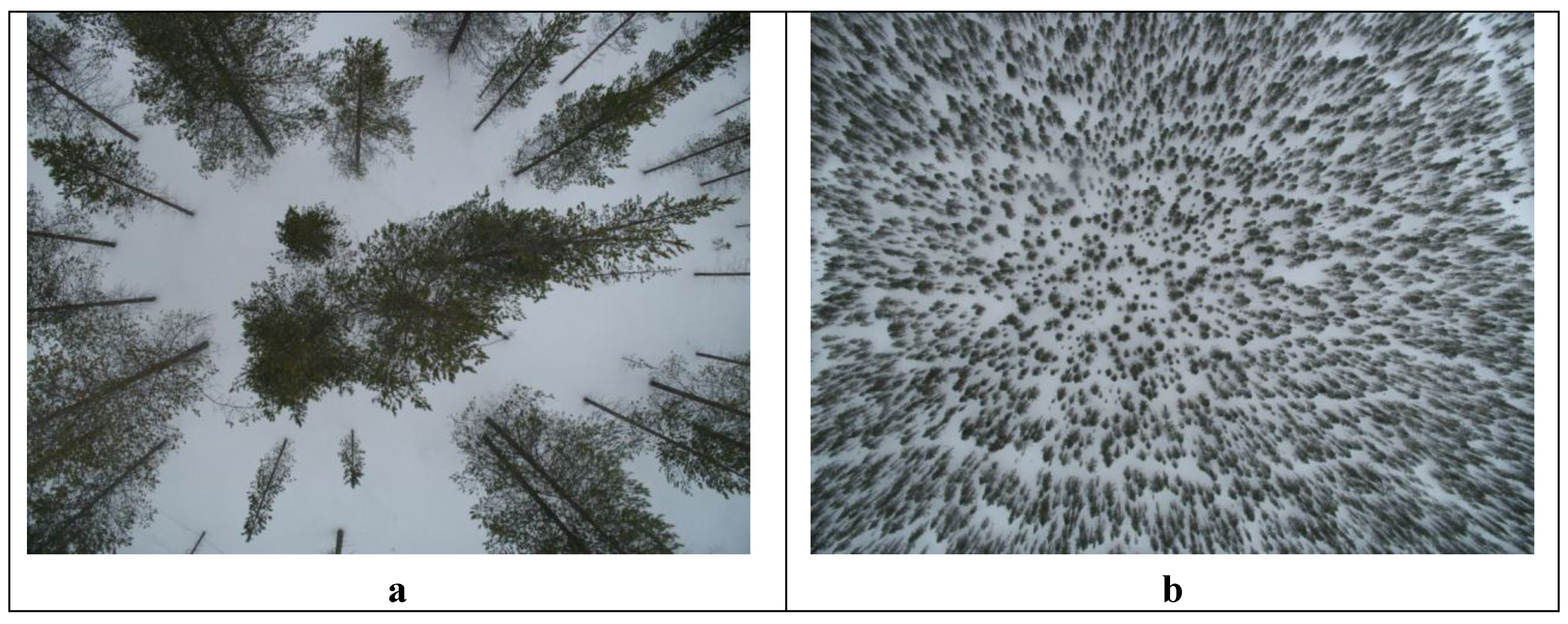
A new airborne method is presented here for leaf area index estimation. The basic technique is the same as used in hemispherical photo analysis [
10,
12]. The difference is just that the background is the snow covered terrain instead of the sky. This naturally limits the use of the technique to the areas with annual snow cover. In addition, the method is not directly suited for broadleaved canopies, which are usually without leaves at the time of the snow cover. Boreal forests are typically dominated by coniferous species and the snow covered season is mostly long. Therefore the method is well suited for LAI estimation of boreal forest and especially useful in the northernmost regions, where the roads are sparse and it is difficult to access the forests scattered between wetlands.
3. Results and Discussion
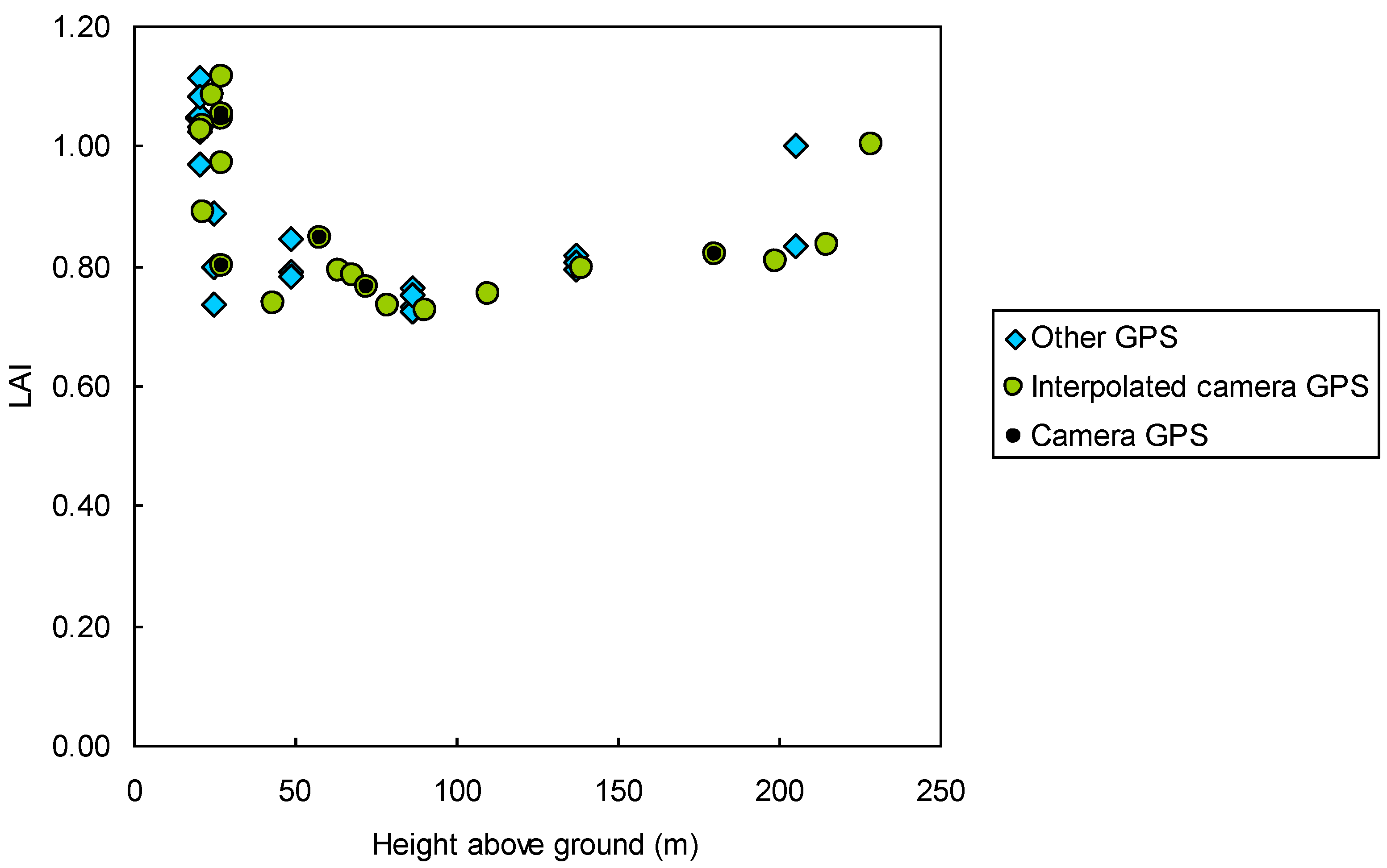
Variation in LAI for different vertical profiles was mainly due to the heterogeneous structure of the forests. When a dense forest patch was surrounded by open areas, LAI decreased with increasing flight altitude, whereas the opposite behaviour was observed when a sparse clearing in a forest was at the centre of the image. Thus it is not trivial, from which altitude the LAI value should be taken to compare with the ground measurements. The forest area detected by the ground based and airborne measurements should be about the same. For LAI-2000 the largest zenith angle is 74°, so that the radius of the area would be about 3.4 times the canopy height. In the Sodankylä region the average tree height measured in 2008 was 13.8 m and the minimum and maximum values 3.2 m and 21 m, respectively. The hemispherical lens has even wider view angle, but the pixels corresponding to the largest view angles were ignored, so that approximately the same area was detected by the hemispherical camera as the LAI-2000 instrument [
20]. To detect the same area with the smaller viewing angle (41°) of the airborne system, the observation height should be about tan(74°)/tan(41°) = 4 times the tree height, which varied in the test area from 13 m to 84 m with an average value of 55 m (
Table 1).
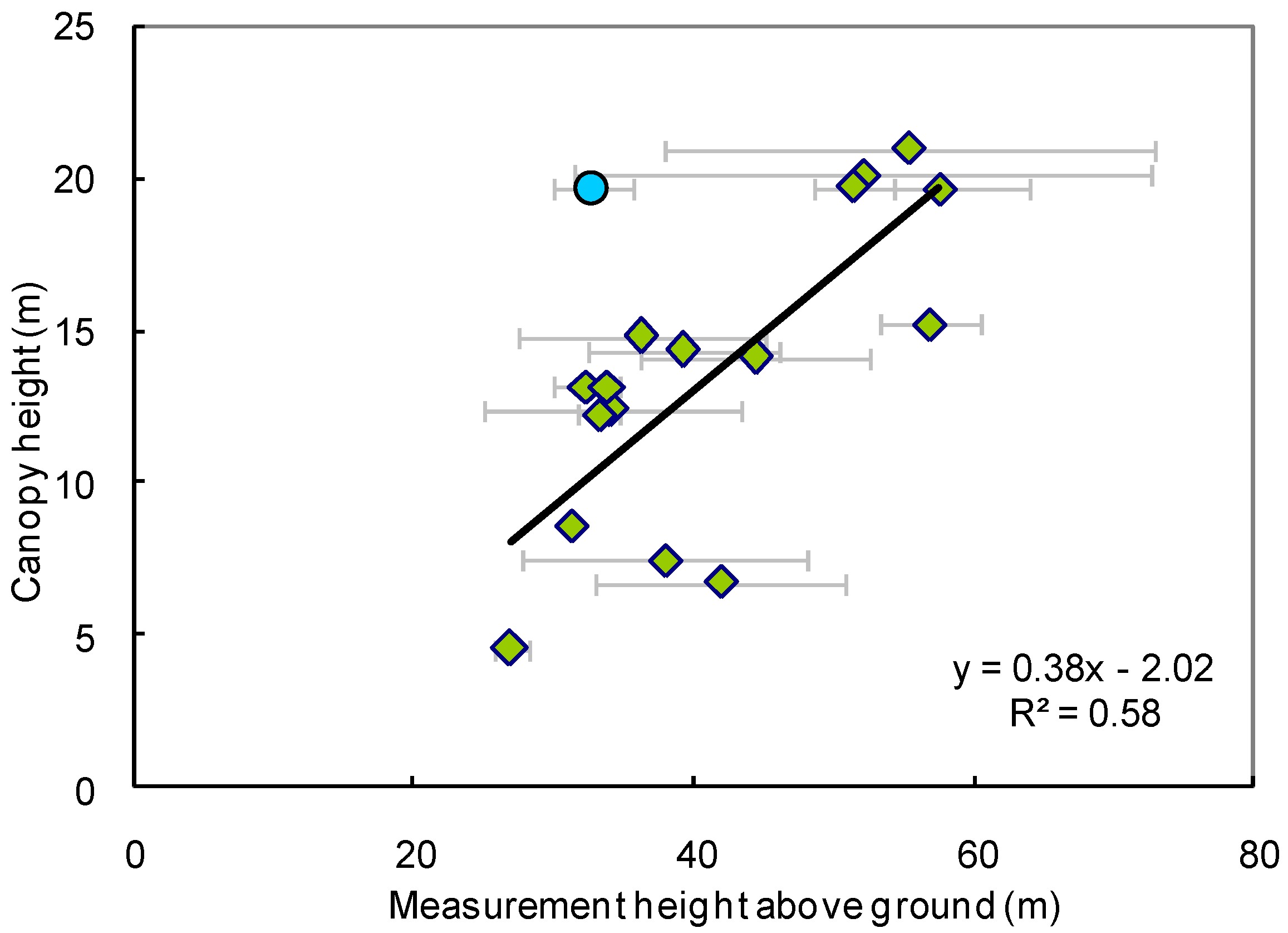
Figure 7.
The relationship of the canopy height and the average altitude of the two GPS systems corresponding to the images to be used for LAI retrieval comparison with ground measurements. The missing GPS height values of the camera system were interpolated before taking the average of the two GPS systems. The terrain height was subtracted from the GPS height values. The GPS heights of the two systems are shown as error bars of the average value. The outlier (blue marker) not included in the regression corresponds to a plot, which was so close to the road, that the LAI values derived from the higher altitudes were deteriorated by that.
The two independent GPS-coordinate data sets were compared and it turned out that the latitude and longitude values were equal with a high precision. The height values, on the contrary, varied on the average 8.4 m with a standard deviation of 9.5 m during the whole flight (which contained 624 height value pairs) although the general trend was the same (R
2 = 0.96). This was due to the different logic of the two measurement systems. The GPS of the camera produced an instantaneous height value on the average for every 12 seconds (
i.e., for every 4
th image), whereas the other GPS provided an average height coordinate value every 10 seconds. The absolute accuracy of the vertical profile heights is not good enough to be used for choosing the image for LAI comparison with ground measurements. Yet the optimal height should increase with increasing canopy height. Therefore all altitudes were also roughly checked by visual inspection of the photos. The GPS heights were given with respect to sea level and the terrain heights obtained from a digital elevation model of 10 m resolution were subtracted from the GPS heights to obtain flight altitudes with respect to the ground. The altitudes of the chosen images were compared to the canopy height values (
Figure 7).
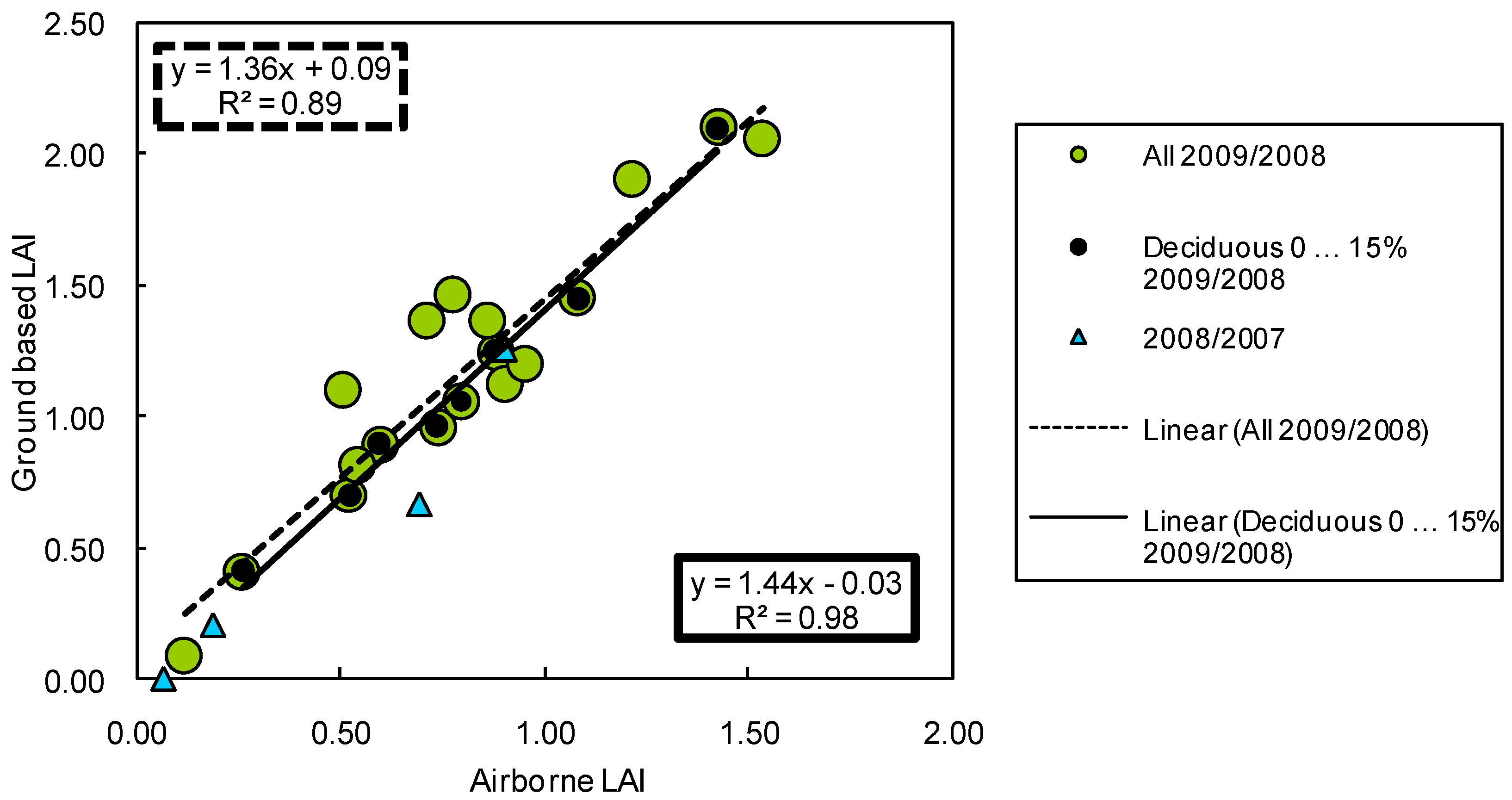
The LAI values derived from the airborne wide optics photos were compared to the stand wise average LAI values obtained from the hemispherical photos taken in the same locations in the previous autumn. In coniferous forest the difference between the leaf area index in summer and winter conditions is not large. For two plots with no deciduous trees the LAI values measured at ground in winter 2008 and in summer 2008 differed only 0.02 and −0.24, although it was not possible to achieve exactly identical geolocation. The comparison results are shown in
Figure 8.
Figure 8.
Relationship of the ground based and airborne LAI values. The airborne values were measured in March 13, 2009 and corresponding ground measurements were carried out during August 26–September 5, 2008 The points for airborne measurements 2008 and ground measurements 2007, for which the airborne location is closer than 30 m to that of the ground measurements and which don’t have deciduous LAI contribution, are shown as well.
The coefficient of determination of the linear regression between the LAI values by the two methods is high (R
2 = 0.89 for all stands and R
2 = 0.98 for coniferous stands) and the offset small. The standard error for the predicted LAI using the airborne LAI was 0.12 for all data and 0.05 for stands with less or equal to 15% deciduous species. However, the slope of the regression lines significantly deviates from unity: the ground based (“true”) LAI was on average 36% (44%) higher than the airborne LAI. The bias in the airborne LAI is explained by the limited zenith angle range of the aerial photos. More precisely, a value of
Gmean = 0.37 (instead of 0.5) for the aerial photos would cause the LAI estimate to differ from its true value by the observed amount.
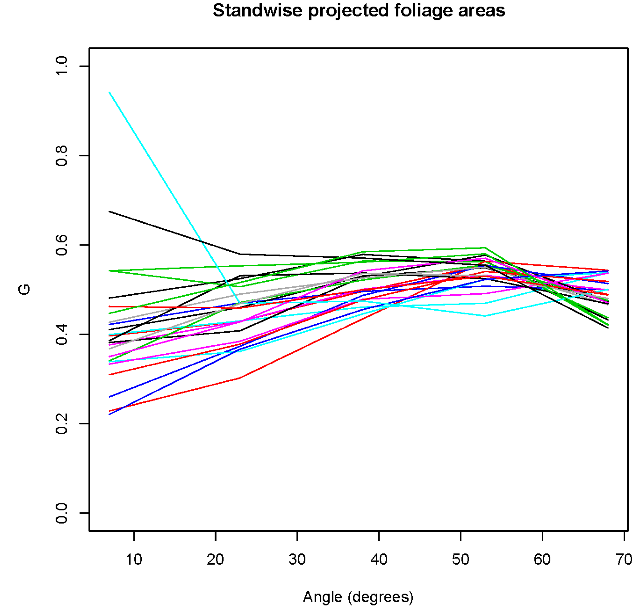
G-values calculated from the ground based hemispherical photos are shown in
Figure 9. At the smallest zenith angle of 7 degrees (corresponding to the mean angle of the uppermost ring of the LAI-2000 instrument), the value of
G averaged 0.4 (excluding the single outlier, a sapling stand), and was dominantly closer to 0.4 than 0.5 throughout the zenith angle range corresponding to that of the aerial photos. Subsequently, when the hemispherical photos (ground data of 2007) were analyzed using only the zenith angle range of the airborne data, the ratio of LAI derived using the full zenith angle range to LAI derived using the smaller zenith angle range was similar to the slope(s) of the regression lines in
Figure 8. For all data, the ratio was on average 1.38 with a standard deviation of 0.55. The ratio for the ground based LAI values (derived using a wide angle range) to the airborne LAI values for 2008/2009 (derived using the small angle range) was on the average 1.47 with a standard deviation of 0.31. When only stands with deciduous contribution up to 15 % were analyzed the ratio was 1.41 with a standard deviation of 0.09.
Figure 9.
Standwise values of the mean projection of unit foliage area (G) as a function of sun zenith angle, calculated from ground based hemispherical photos of 2008.
Figure 9.
Standwise values of the mean projection of unit foliage area (G) as a function of sun zenith angle, calculated from ground based hemispherical photos of 2008.
In addition, even if the cross sectional area of the canopy covered by the airborne and ground based photos were equal the part of the canopy detected would not be equal due to the conical viewing geometry (when fully hemispherical viewing is not applied). The airborne photos will then contain at the edges only lower parts of the trees, whereas the ground based photos will see only the top part of the same trees. Therefore the airborne LAI estimate inevitably tends to be slightly smaller than the ground based estimate, especially for Scots pine, the crown of which can be located altogether very high up.
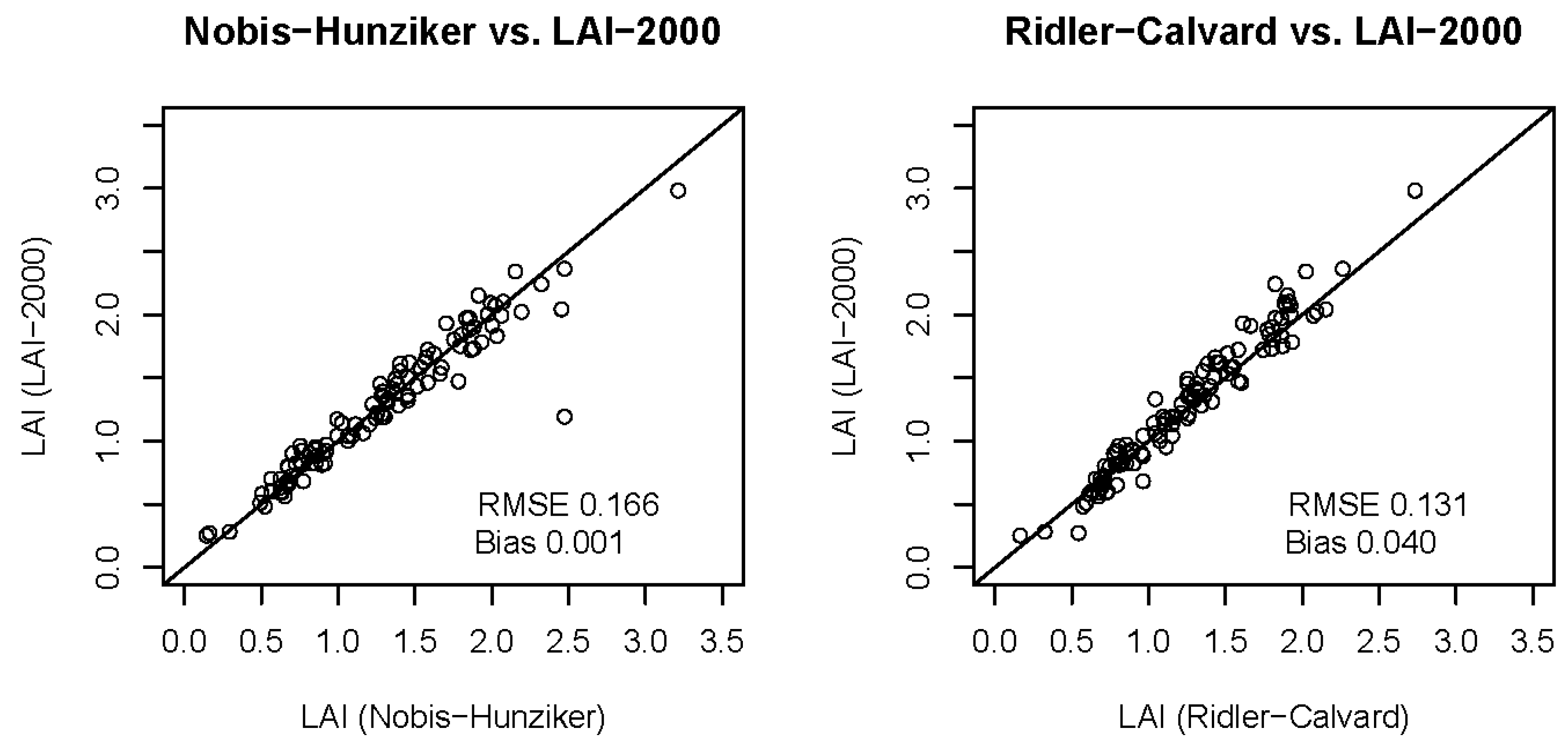
Taking into account that the LAI correlation of two different ground based methods (LAI-2000 and hemispherical photos) had a root mean square error of 0.131…0.166 (
Figure 3), the difference between the airborne and ground based LAI value is of the order of the measurement method accuracy of hemispherical photos. Judging from that the coefficient of determination of the relationship between ground based and airborne LAI for purely coniferous stands is very high (
Figure 9), the effect of the decreased zenith angle range is the same for all canopies in the studied area,
i.e., they have similar
G-values in the zenith angle range covered by the aerial photos. If this turns out to be more generally true, the linear coefficient has to be calibrated empirically once, but then it can be used for the same kind of forests as long as the airborne camera system remains the same.
When the regression line of
Figure 8 comprising all data points was applied to the airborne data (to scale them to the level of the ground data), the average difference between the LAI values of the two data sets was 0.14 for the whole data and 0.06 for stands with up to 15% deciduous trees. The three obvious airborne LAI underestimates seen in
Figure 8 were obtained in stands with a larger fraction of deciduous trees among the coniferous species, which naturally decreases the LAI value in winter (airborne) from that obtained in the autumn (ground based) (
Figure 10). The results of 2008/2007 are deteriorated due to the mismatch of the location of the airborne and ground based measurements, which was obvious also from the images.
Figure 10.
LAI is underestimated in forests with large percentage of deciduous trees.
Figure 10.
LAI is underestimated in forests with large percentage of deciduous trees.
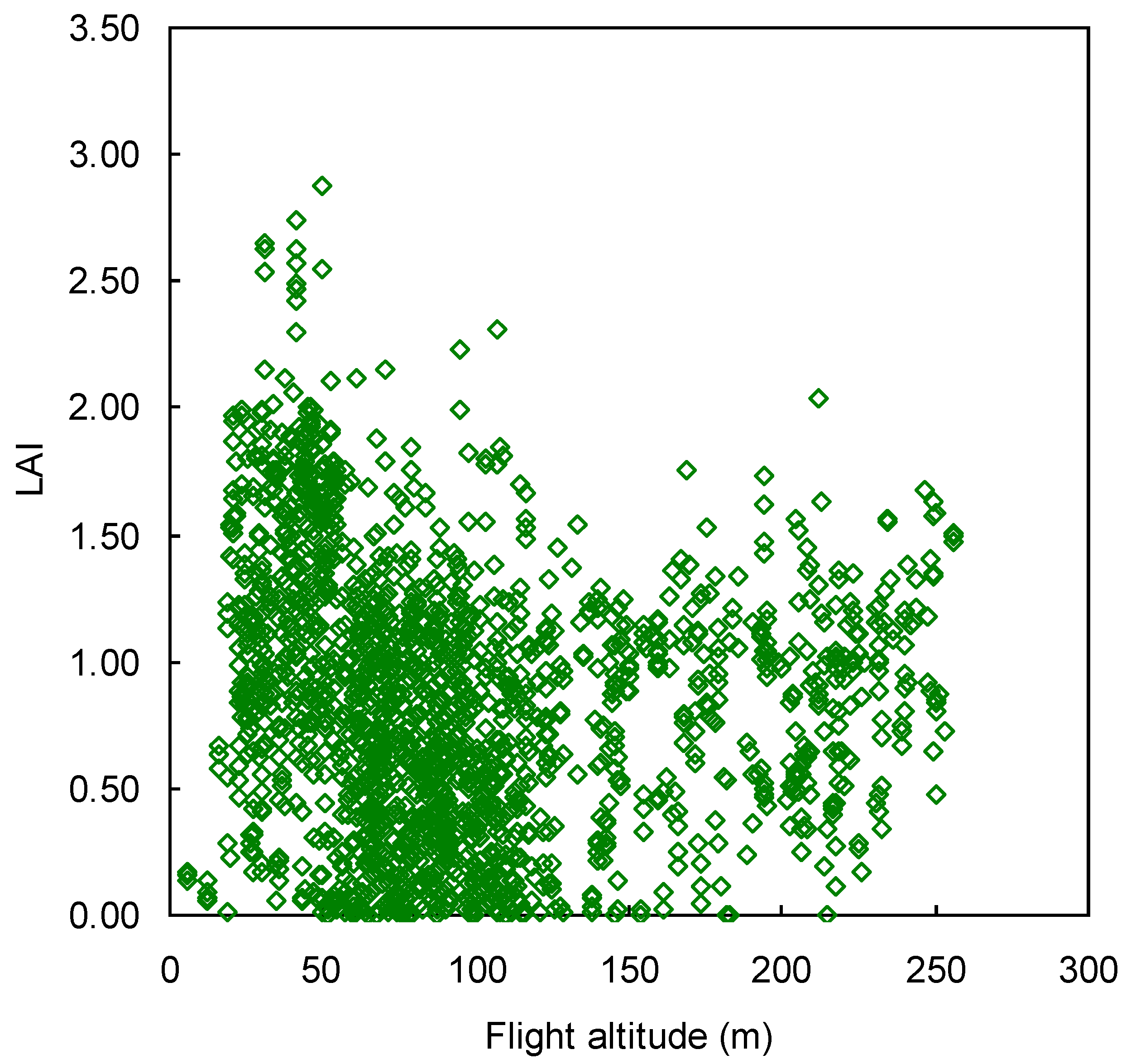
The measured LAI values depend on the flight altitude. The lower the altitude is the smaller is the area seen by the camera and the larger is the variation of diverse scenes, whereas high altitude flights produce more averaged LAI values. The range of variation in LAI with varying flight altitude is shown in
Figure 11 for all points acquired March 13, 2009. The data contains the vertical profiles and the horizontal flights between the successive profile locations. Obviously the maximum LAI value decreases markedly when the flight altitude increases from the tree tops to about 100 m. There is no single optimal flight altitude to derive LAI estimates. If one is interested in characterizing small forest stands, the flight altitude should be chosen so that the image area matches about that of typical ground measurements. On the other hand, if one is interested in comparing the values with satellite based LAI estimates it might be more useful to cover the area of a satellite pixel, so that both instruments would directly measure the same target area. However, one has to take into account that the resolution decreases with increasing flight altitude, so that the detection of gaps inside crowns may not be possible after some critical altitude. Further studies and comparison with satellite based LAI estimates are needed to find the optimal flight altitude range.
Figure 11.
The observed LAI value versus the flight altitude above ground in March 13, 2009. The values are scaled using the regression line of
Figure 8 for all data points of 2009.
Figure 11.
The observed LAI value versus the flight altitude above ground in March 13, 2009. The values are scaled using the regression line of
Figure 8 for all data points of 2009.
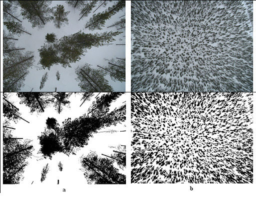
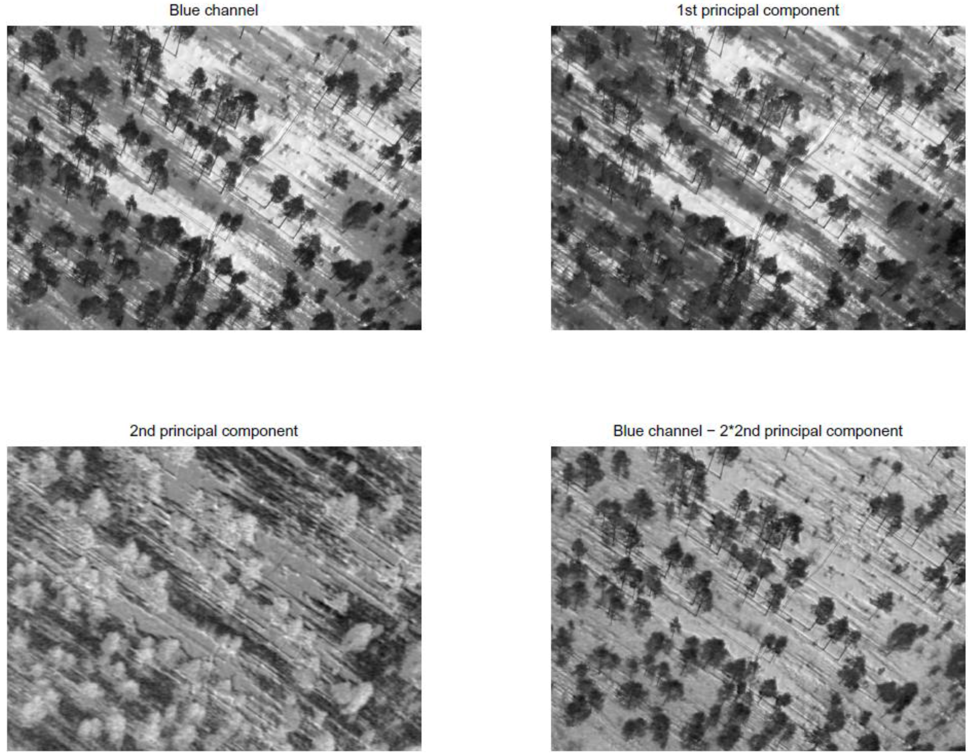
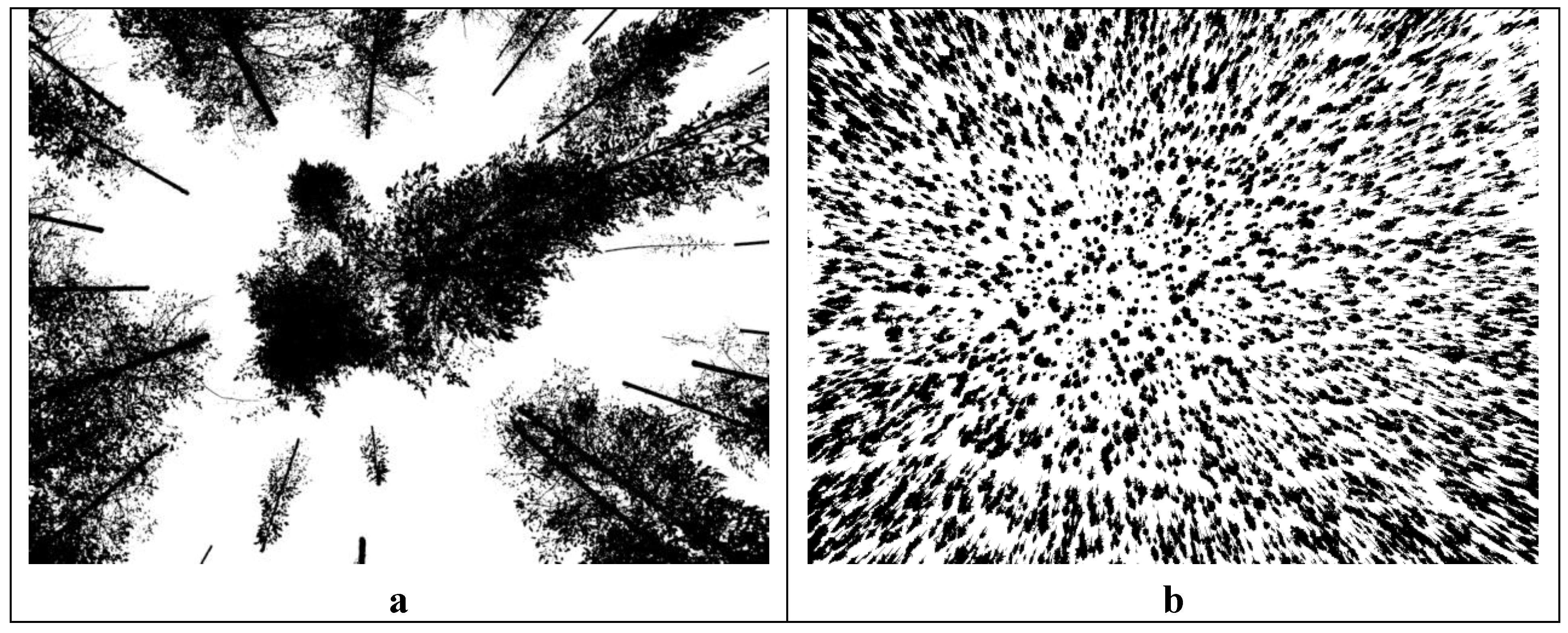
The derived LAI retrieval method is well suited to areas with difficult accessibility at ground level. Cloudy weather is better than sunny, because then there are no obvious shadows at the forest floor. However, the shadows can be removed using the principal component analysis (
Figure 2) [
17]. The snow cover at the forest floor makes a good background, but no snow on the trees can be accepted.


