Operating Strategy for Local-Area Energy Systems Integration Considering Uncertainty of Supply-Side and Demand-Side under Conditional Value-At-Risk Assessment

Abstract
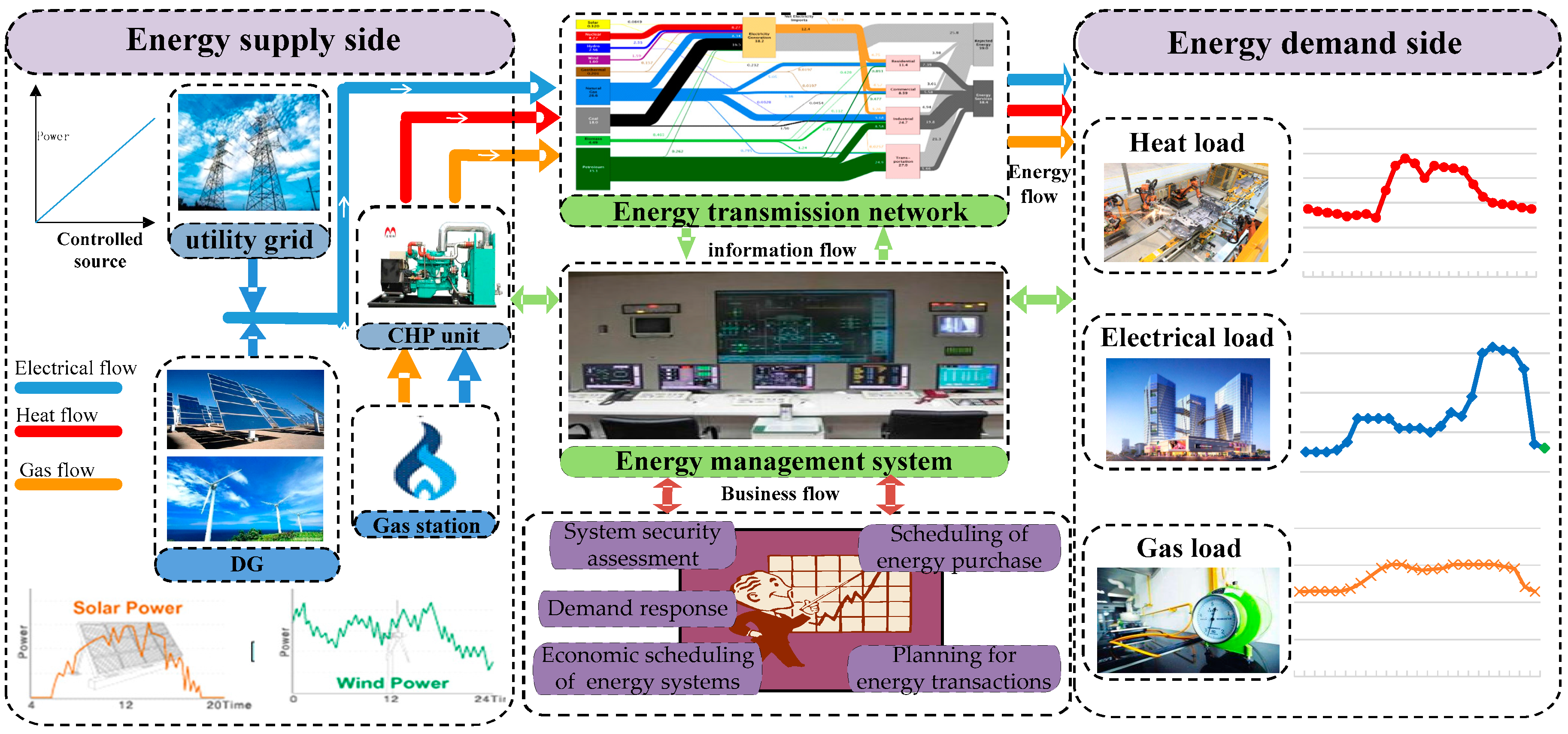
:1. Introduction
- (1)
- To the best of our knowledge, the CVaR as risk evaluation approach has rarely been applied in local-area ESI operating strategy research. In this paper, risk assessment of local-area ESI is proposed to quantify the impact occurred by uncertainty of energy supply-side and demand-side.
- (2)
- In the modeling process, risk cost, which includes the fuel cost, maintenance cost and facility adjustment cost, is especially analyzed in the case of overestimation and underestimation as multiple sources of energy interact, and constraints of multi-energy systems network are fully taken into account.
- (3)
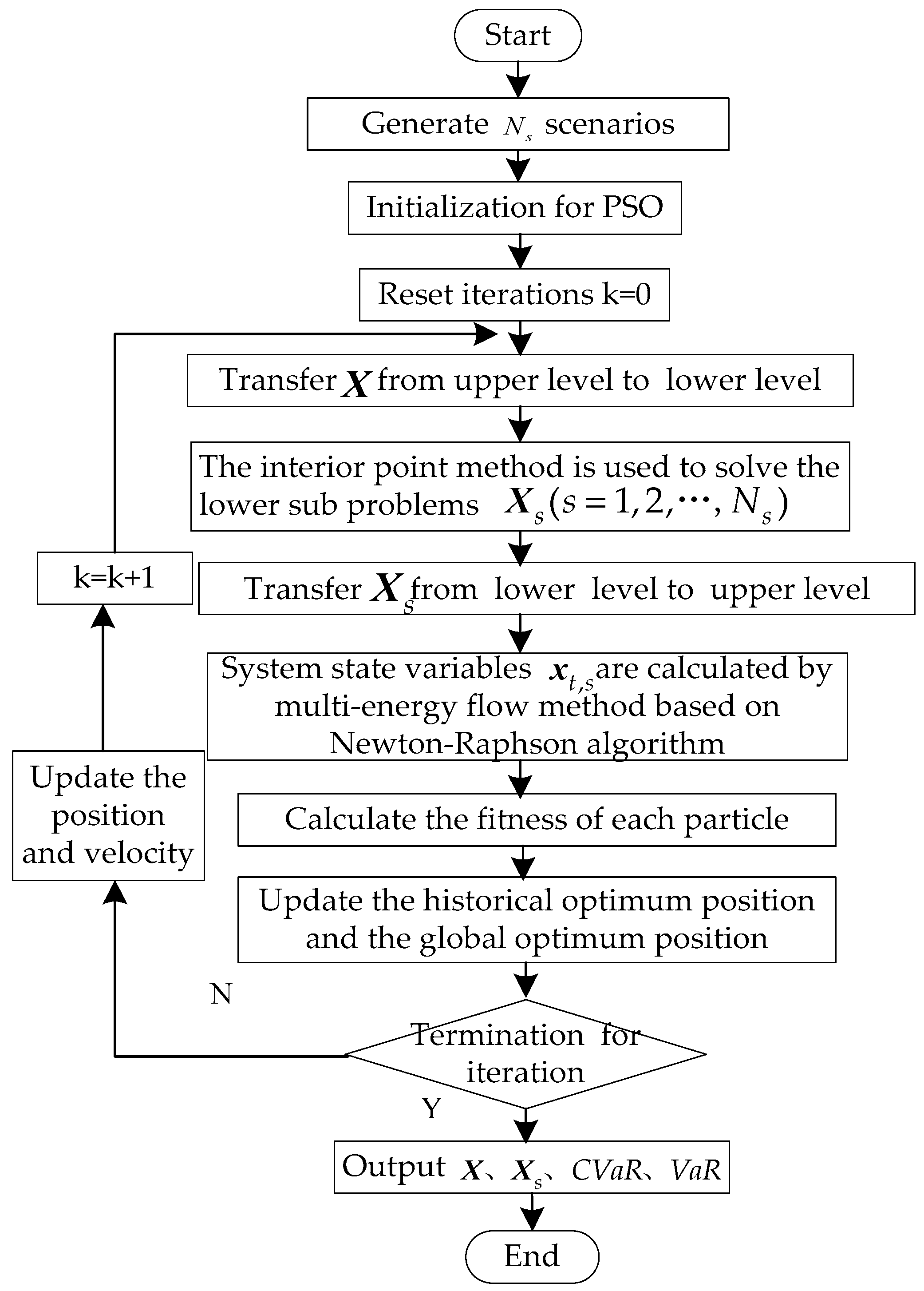
- By considering the advantage of the algorithm and the complexity of the ESI model, a bi-level optimization algorithm which combines particle swarm optimization (PSO) approach with interior point (IP) method is used to solve the stochastic multi-period mixed-integer model for dispatching issue.
2. Mathematical Model Formulation
2.1. Mathematical Model of Electricity Supply Equipment in Local-Area ESI
2.1.1. Micro Turbine CHP Model
2.1.2. Fuel Cell Model
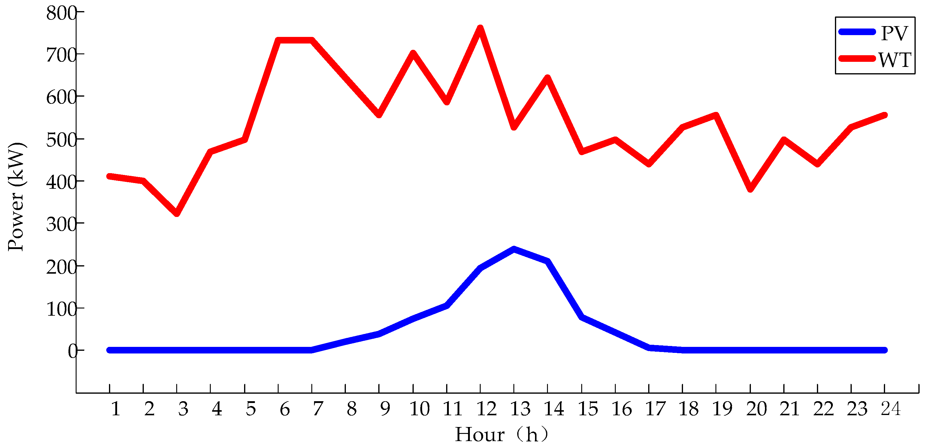
2.1.3. Photovoltaic Power Generation Model
2.1.4. Wind Power Generation Model
2.2. Mathematical Model of Heat Supply Equipment in Local-Area ESI
2.2.1. Ground Source Heat Pump Model
2.2.2. Gas Boiler Model
2.3. Uncertainty Analysis in Local-Area IES
2.3.1. Uncertainty of Energy Supply Side
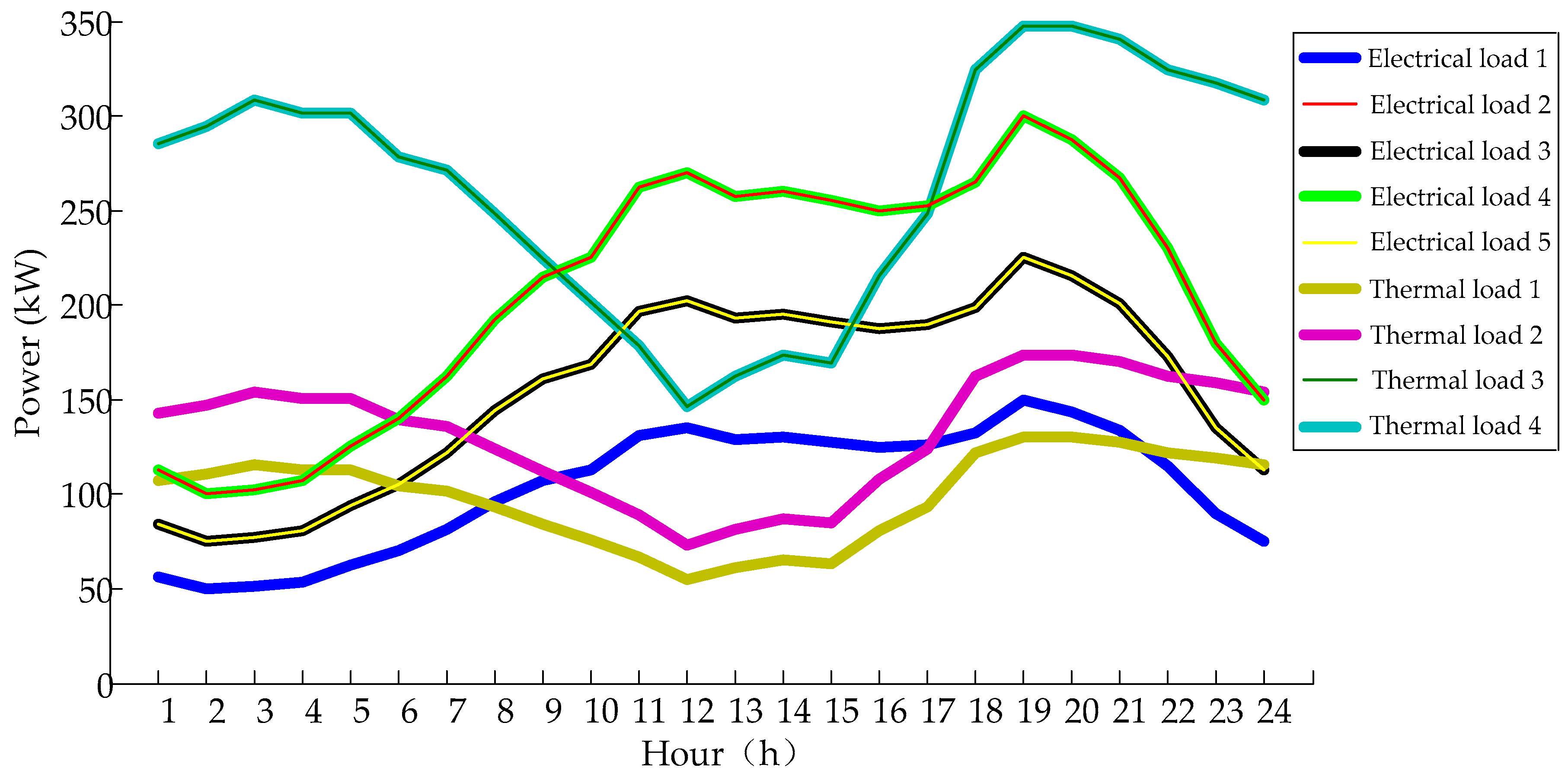
2.3.2. Uncertainty of Energy Demand Side
2.3.3. Reduction of Uncertainty Scenarios
3. CVaR Based Dispatching Model for Local-Area ESI
3.1. Risk Modelling via CVaR
3.2. Risk Cost of ESI
3.2.1. Overestimated Cost
Overestimated Cost for Electricity
Overestimated Cost for Heat
3.2.2. Underestimated Cost
Underestimated Cost for Electricity
Underestimated Cost for Heat
3.2.3. Total Cost
3.3. Objective and Constraint of ESI Economic Dispatch
3.3.1. Objective Function
3.3.2. Constraint Conditions
The Upper and Lower Bound of Energy Supply Equipment Output
Power Balance Constraints
Tie-Line Power Constraints
Ramping Rate Constraints
Multi-Energy Flow Constraints
System State Variables Constraints
3.4. Solving Algorithm
Upper Level Optimization Model
Lower Level Optimization Model
4. Case Study
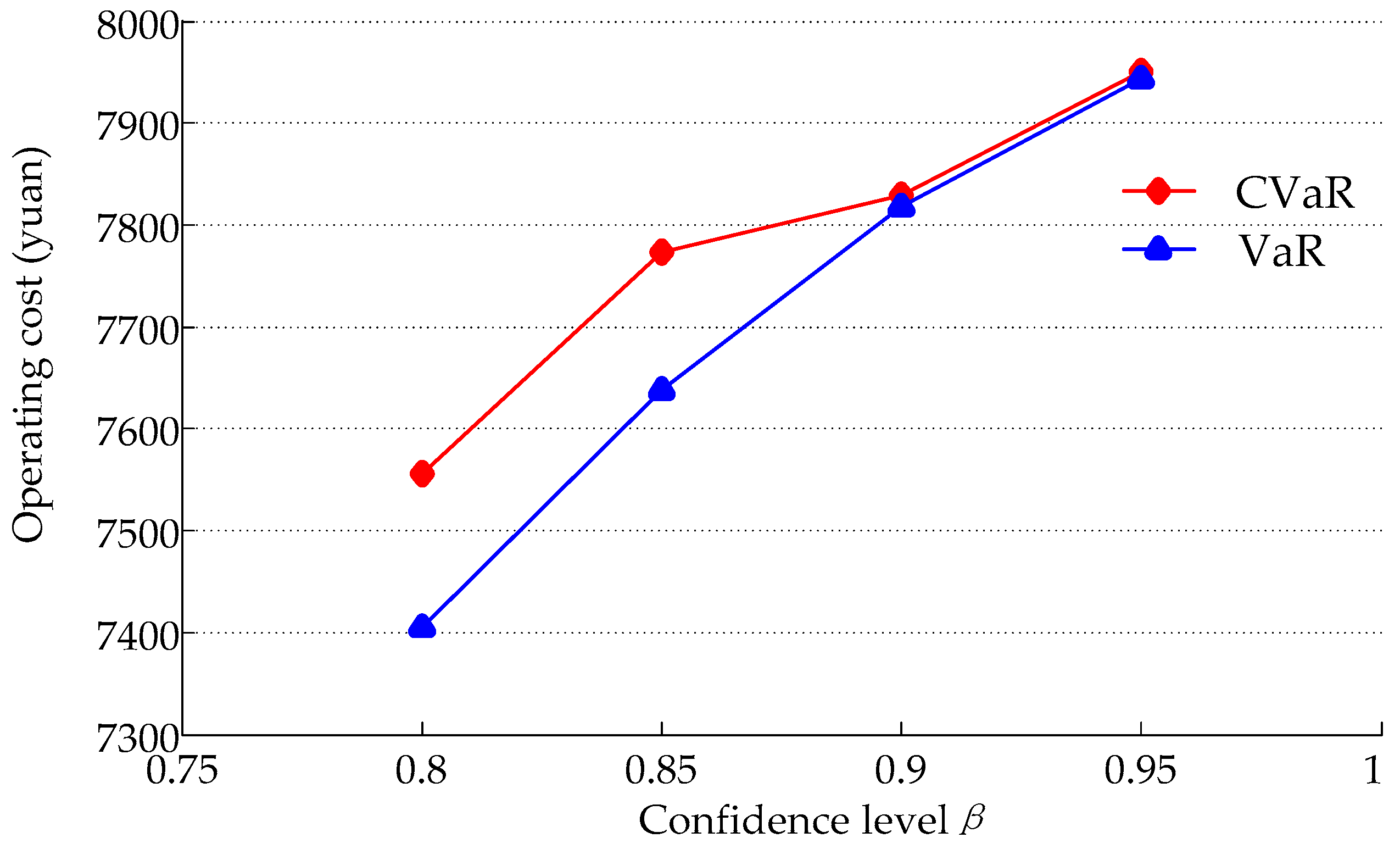
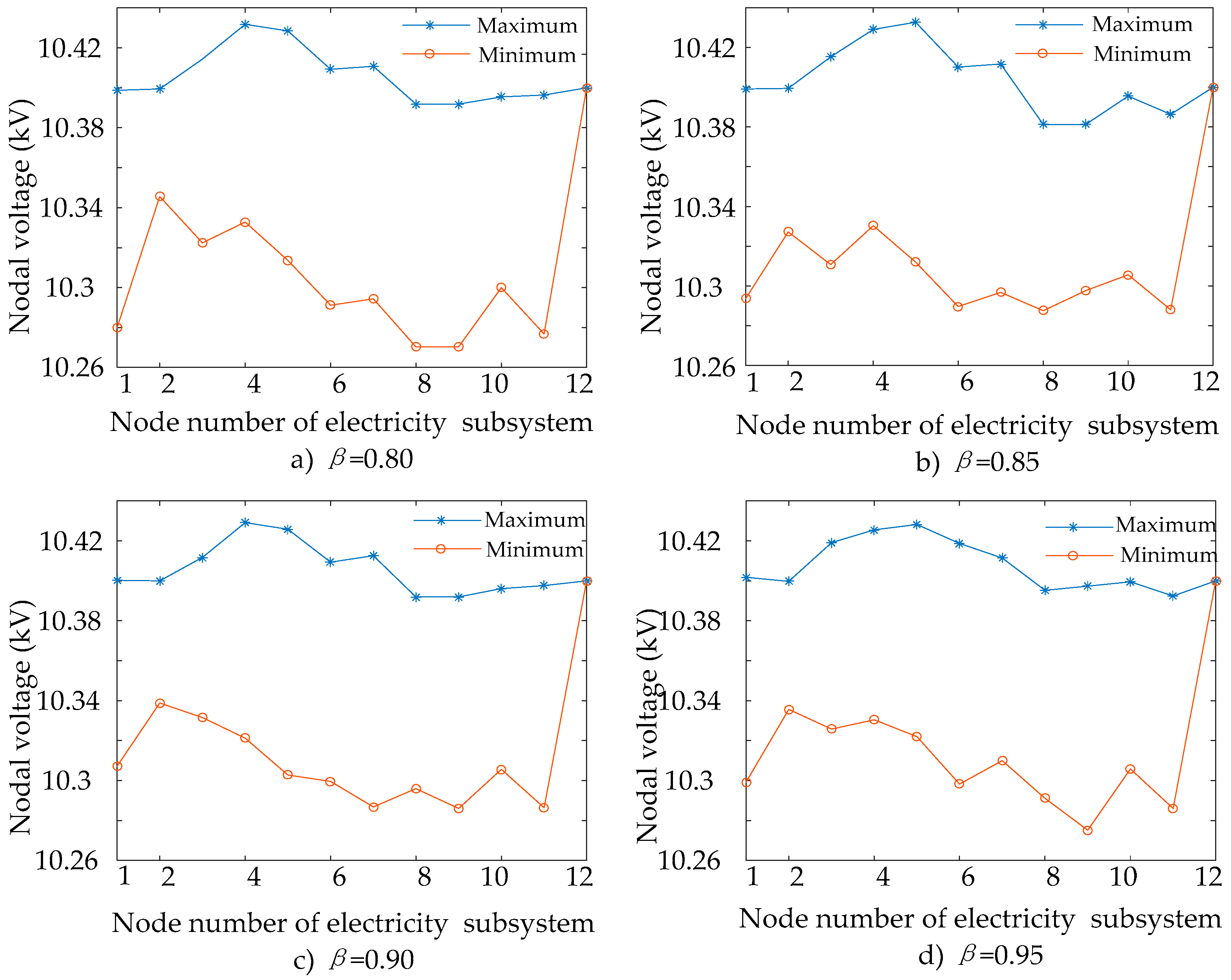
4.1. Simulation Based on Different Confidence Level
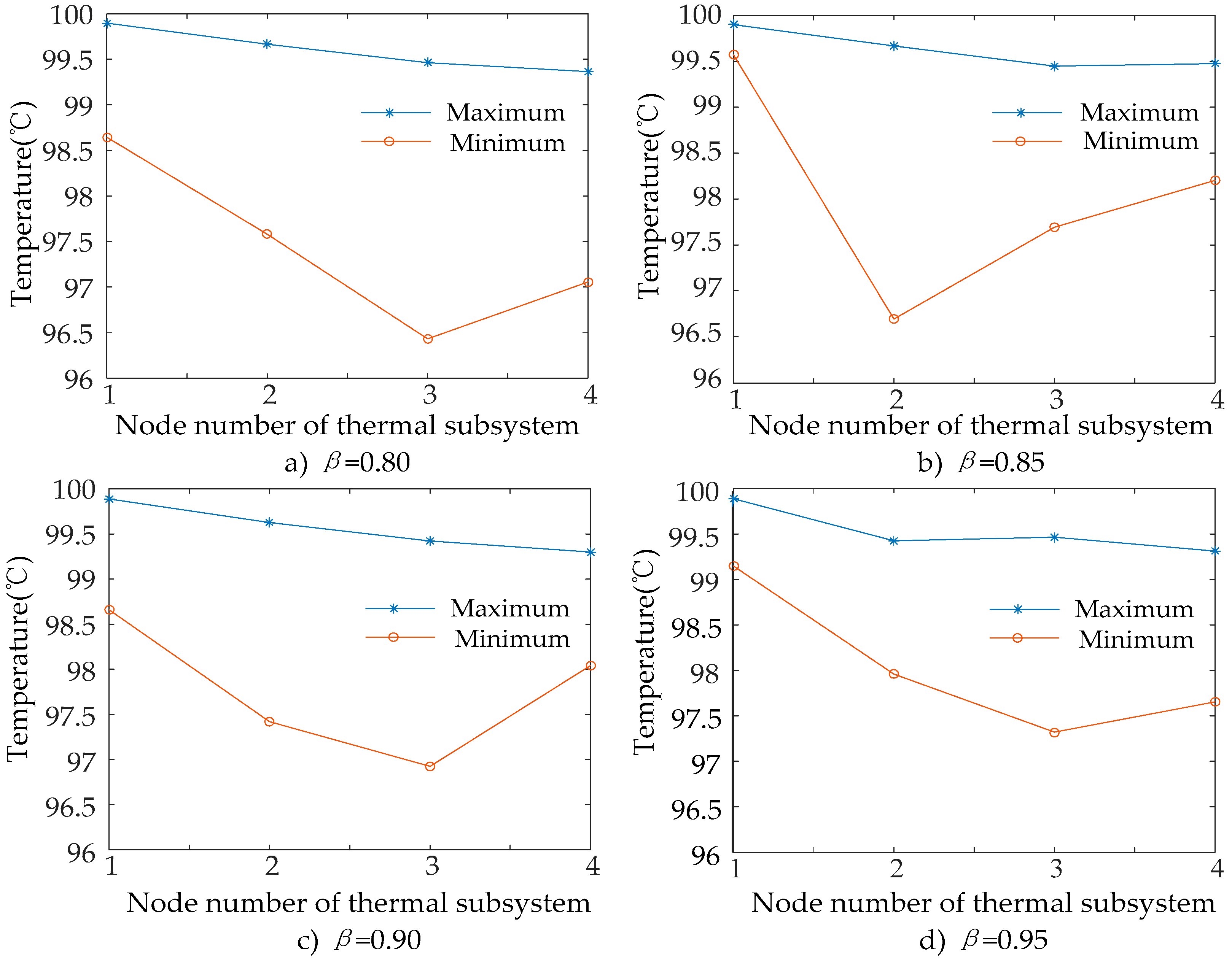
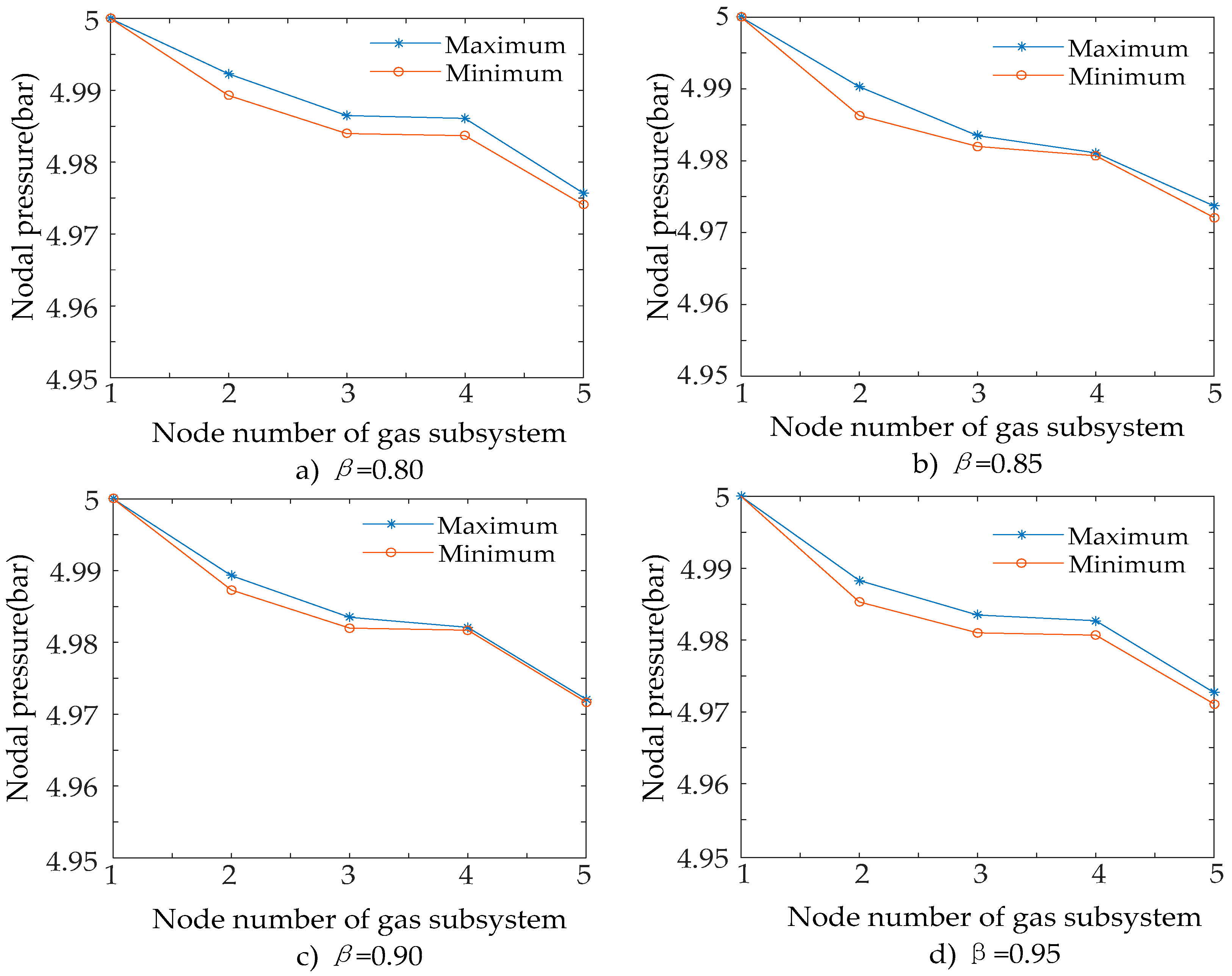
4.2. The Influence of Multi-Energy Flow Constraints on Simulation Results
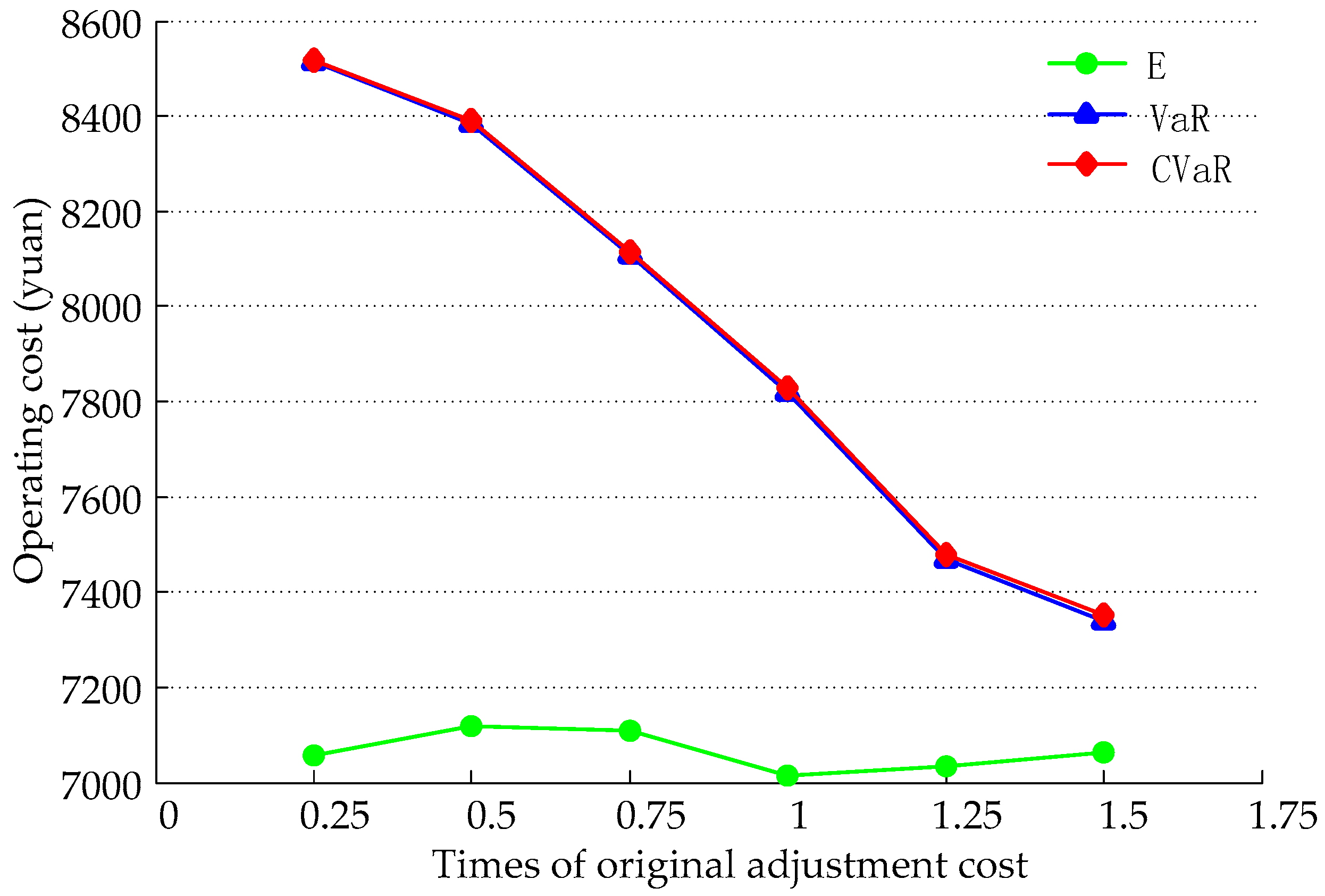
4.3. The Influence of Equipment Adjustment Cost on Simulation Results
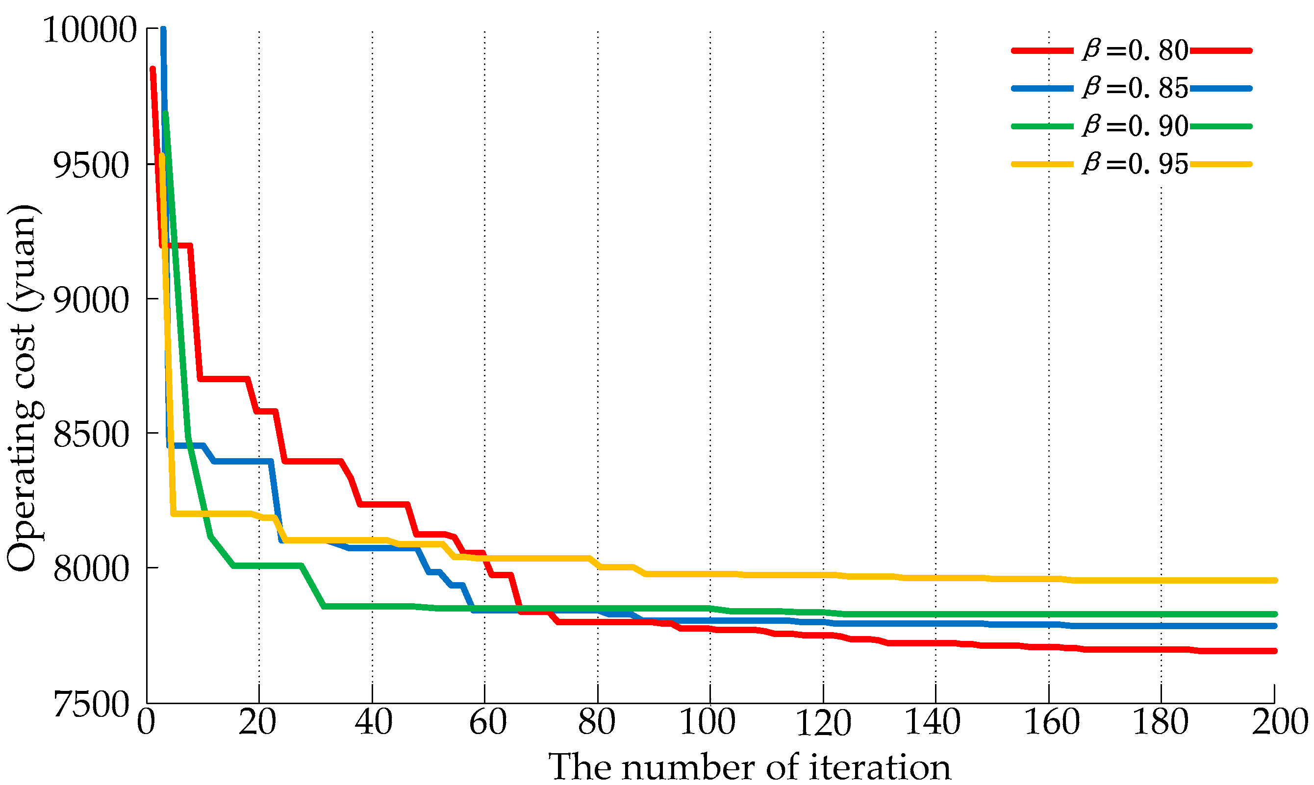
4.4. Convergence Analysis
5. Conclusions
Acknowledgments
Author Contributions
Conflicts of Interest
Appendix A

| Equipment Name | Minimum Power Output (kW) | Maximum Power Output (kW) | Ramping up Rate (kW/min) | Ramping down Rate (kW/min) | Maintenance Cost (Yuan/kW) |
|---|---|---|---|---|---|
| CHP | 5 | 130 | 5 | 10 | 0.0149 |
| FC | 10 | 200 | 10 | 10 | 0.009 |
| GSHP | 0 | 200 | 5 | 5 | 0.0311 |
| GB | 100 | 1500 | 5 | 6 | 0.025 |
| Utility grid | −600 | 600 | - | - | - |
Appendix B
| Direction of Line | Length (m) | Direction of Line | Length (m) |
|---|---|---|---|
| 12–2 | 50 | 2–10 | 50 |
| 2–3 | 130 | 8–9 | 100 |
| 3–4 | 100 | 10–9 | 100 |
| 4–5 | 100 | 11–10 | 100 |
| 3–6 | 100 | 1–11 | 50 |
| 7–6 | 100 | - | - |
| Direction of Pipeline | Length (m) | Diameter (mm) | Direction of Pipeline | Length (m) | Diameter (mm) |
|---|---|---|---|---|---|
| 4–3 | 50 | 100 | 1–2 | 150 | 100 |
| 5–3 | 100 | 100 | 7–1 | 100 | 100 |
| 2–4 | 150 | 100 | 6–4 | 50 | 100 |
| Direction of Pipeline | Length (m) | Diameter (mm) | Direction of Pipeline | Length (m) | Diameter (mm) |
|---|---|---|---|---|---|
| 1–2 | 100 | 200 | 3–4 | 100 | 200 |
| 2–3 | 300 | 200 | 3–5 | 350 | 200 |
References
- Rifkin, J. The Third Industrial Revolution; Zhang, T.W., Sun, Y.L., Eds.; CITIC Press: Beijing, China, 2012. [Google Scholar]
- Shiming, T.; Wenpeng, L.; Dongxia, Z.; Caihao, L.; Yaojie, S. Technical Forms and Key Technologies on Energy Internet. Proc. CSEE 2015, 35, 3482–3494. [Google Scholar]
- Sun, Q.; Wang, B.; Huang, B.; Ma, D. The Optimization Control and Implementation for the Special Energy Internet. Proc. CSEE 2015, 35, 4571–4580. [Google Scholar]
- Parisio, A.; Vecchio, C.D.; Vaccaro, A. A robust optimization approach to energy hub management. Int. J. Electr. Power Energy Syst. 2012, 42, 98–104. [Google Scholar] [CrossRef]
- Qadrdan, M.; Wu, J.; Jenkins, N.; Ekanayake, J. Operating Strategies for a GB Integrated Gas and Electricity Network Considering the Uncertainty in Wind Power Forecasts. IEEE Trans. Sustain. Energy 2014, 5, 128–138. [Google Scholar] [CrossRef]
- Alabdulwahab, A.; Abusorrah, A.; Zhang, X.; Shahidehpour, M. Coordination of Interdependent Natural Gas and Electricity Infrastructures for Firming the Variability of Wind Energy in Stochastic Day-Ahead Scheduling. IEEE Trans. Sustain. Energy 2015, 6, 606–615. [Google Scholar] [CrossRef]
- Bai, L.; Li, F.; Cui, H.; Jiang, T.; Sun, H.; Zhu, J. Interval optimization based operating strategy for gas-electricity integrated energy systems considering demand response and wind uncertainty. Appl. Energy 2016, 167, 270–279. [Google Scholar] [CrossRef]
- Zhang, X.; Shahidehpour, M.; Alabdulwahab, A.S.; Abusorrah, A. Security-Constrained Co-Optimization Planning of Electricity and Natural Gas Transportation Infrastructures. IEEE Trans. Power Syst. 2015, 30, 2984–2993. [Google Scholar] [CrossRef]
- Garcia-Bertrand, R. Sale prices setting tool for retailers. IEEE Trans. Smart Grid 2013, 4, 2028–2035. [Google Scholar] [CrossRef]
- Morales, J.M.; Conejo, A.J.; Perez-Ruiz, J. Short-term trading for a wind power producer. IEEE Trans. Power Syst. 2010, 25, 554–564. [Google Scholar] [CrossRef]
- Catalao, J.P.S.; Pousinho, H.M.I.; Mendes, V.M.F. Optimal offering strategies for wind power producers considering uncertainty and risk. IEEE Syst. J. 2012, 6, 270–277. [Google Scholar] [CrossRef]
- Baringo, L.; Conejo, A.J. Risk-constrained multi-stage wind power investment. IEEE Trans. Power Syst. 2013, 28, 401–411. [Google Scholar] [CrossRef]
- Safdarian, A.; Fotuhi-Firuzabad, M.; Lehtonen, M. A stochastic framework for short-term operation of a distribution company. IEEE Trans. Power Syst. 2013, 28, 4712–4721. [Google Scholar] [CrossRef]
- Lu, G.; Wen, F.; Chung, C.Y.; Wong, K.P. Conditional value-a trisk based mid-term generation operation planning in electricity market environment. In Proceedings of the IEEE Congress on Evolutionary Computation, Singapore, 25–28 September 2007; pp. 2745–2750. [Google Scholar]
- Zhang, Y.; Giannakis, G.B. Robust optimal power flow with wind integration using conditional value-at-risk. In Proceedings of the IEEE Smart Grid Communications, Vancouver, BC, Canada, 21–24 October 2013; pp. 654–659. [Google Scholar]
- Al-Awami, A.T.; El-Sharkawi, M.A. Coordinated trading of wind and thermal energy. IEEE Trans. Sustain. Energy 2011, 2, 277–287. [Google Scholar] [CrossRef]
- De la Nieta, A.A.S.; Contreras, J.; Munoz, J.I. Optimal coordinated wind-hydro bidding strategies in day-ahead markets. IEEE Trans. Power Syst. 2013, 28, 798–809. [Google Scholar] [CrossRef]
- Le, L.I. Study on Economic Operation of Microgrid. Master’s Thesis, North China Electric Power University, Beijing, China, June 2011. [Google Scholar]
- Sharma, S.; Pollet, B.G. Support materials for PEMFC and DMFC electrocatalysts—A review. J. Power Sources 2012, 208, 96–119. [Google Scholar] [CrossRef]
- Terhan, M.; Comakli, K. Energy and exergy analyses of natural gas-fired boilers in a district heating system. Appl. Therm. Eng. 2017, 121, 380–387. [Google Scholar] [CrossRef]
- Sivasakthivel, T.; Murugesan, K.; Sahoo, P.K. Optimization of ground heat exchanger parameters of ground source heat pump system for space heating applications. Energy 2014, 78, 573–586. [Google Scholar] [CrossRef]
- Wang, J.; Shahidehpour, M.; Li, Z. Security-Constrained Unit Commitment with Volatile Wind Power Generation. IEEE Trans. Power Syst. 2008, 23, 1319–1327. [Google Scholar] [CrossRef]
- Nguyen, D.T.; Le, L.B. Risk-Constrained Profit Maximization for Microgrid Aggregators with Demand Response. IEEE Trans. Smart Grid 2015, 6, 135–146. [Google Scholar] [CrossRef]
- Gao, Y.; Li, R.; Liang, H.; Zhang, J.; Ran, J.; Zhang, F. Two step optimal dispatch based on multiple scenarios technique considering uncertainties of intermittent distributed generations and loads in the active distribution system. Proc. Chin. Soc. Electr. Eng. 2015, 35, 1657–1665. [Google Scholar]
- Deng, C.; Ju, L.; Liu, J.; Tan, Z. Stochastic scheduling multi-objective optimization model for hydro-thermal power systems based on fuzzy CVaR theory. Power Syst. Technol. 2016, 40, 1447–1454. [Google Scholar]
- Uryasev, S. Conditional value-at-risk: Optimization algorithms and applications. In Proceedings of the IEEE Computational Intelligence for Financial Engineering, New York, NY, USA, 28 March 2000; pp. 49–57. [Google Scholar]
- Rockafellar, R.T.; Uryasev, S. Conditional value-at-risk for general loss distributions. J. Bank. Financ. 2002, 26, 1443–1471. [Google Scholar] [CrossRef]
- Zhang, F.; Duan, Y.; Qiu, J.; Feng, X.-Q. Research on reactive power flow based on particle swarm optimization and interior point method. Power Syst. Prot. Control 2010, 38, 11–16. [Google Scholar]
- Shi, J.; Wang, L.; Wang, Y.; Zhang, J. Generalized Energy Flow Analysis Considering Electricity Gas and Heat Subsystems in Local-Area Energy Systems Integration. Energies 2017, 10, 514. [Google Scholar] [CrossRef]
- Liu, B.; Wang, L.; Jin, Y.H. An Effective PSO-Based Memetic Algorithm for Flow Shop Scheduling. IEEE Trans. Syst. Man Cybern. Part B Cybern. 2007, 37, 18–27. [Google Scholar] [CrossRef]
- Yu, W. Case Analysis and Application of Optimization Algorithm by MATLAB; Tsinghua University Press: Beijing, China, 2015; pp. 174–179. [Google Scholar]


| Name | Peak Period | Normal Period | Valley Period |
|---|---|---|---|
| Period | 10:00–15:00 18:00–21:00 | 7:00–10:00 15:00–18:00 21:00–23:00 | 23:00–7:00 |
| Electricity purchasing price (Yuan/kWh) | 0.83 | 0.49 | 0.17 |
| Electricity Selling price (Yuan/kWh) | 0.65 | 0.38 | 0.13 |
| β | Electrical Power Output (kWh) | Thermal Power Output (kWh) | |||
|---|---|---|---|---|---|
| CHP | FC | Grid | GSHP | GB | |
| 0.80 | 1741.5 | 2759.4 | 2012.1 | 2287.1 | 13,642.0 |
| 0.85 | 2028.2 | 2527.0 | 1953.1 | 2265.9 | 13,291.0 |
| 0.90 | 1607.8 | 2727.7 | 2336.0 | 3000.4 | 13,103.0 |
| 0.95 | 1738.0 | 2091.0 | 2831.1 | 2949.0 | 12,985.0 |
© 2017 by the authors. Licensee MDPI, Basel, Switzerland. This article is an open access article distributed under the terms and conditions of the Creative Commons Attribution (CC BY) license (http://creativecommons.org/licenses/by/4.0/).
Share and Cite
Shi, J.; Wang, Y.; Fu, R.; Zhang, J. Operating Strategy for Local-Area Energy Systems Integration Considering Uncertainty of Supply-Side and Demand-Side under Conditional Value-At-Risk Assessment. Sustainability 2017, 9, 1655. https://doi.org/10.3390/su9091655
Shi J, Wang Y, Fu R, Zhang J. Operating Strategy for Local-Area Energy Systems Integration Considering Uncertainty of Supply-Side and Demand-Side under Conditional Value-At-Risk Assessment. Sustainability. 2017; 9(9):1655. https://doi.org/10.3390/su9091655
Chicago/Turabian StyleShi, Jiaqi, Yingrui Wang, Ruibin Fu, and Jianhua Zhang. 2017. "Operating Strategy for Local-Area Energy Systems Integration Considering Uncertainty of Supply-Side and Demand-Side under Conditional Value-At-Risk Assessment" Sustainability 9, no. 9: 1655. https://doi.org/10.3390/su9091655
APA StyleShi, J., Wang, Y., Fu, R., & Zhang, J. (2017). Operating Strategy for Local-Area Energy Systems Integration Considering Uncertainty of Supply-Side and Demand-Side under Conditional Value-At-Risk Assessment. Sustainability, 9(9), 1655. https://doi.org/10.3390/su9091655