1. Introduction
Energy is considered a key element in economic growth. Its usage has become a serious alarm in recent years because of a fast rise in energy demand. Besides, environmental problems of traditional energy resources such as climate change and global warming are constantly pushing us for alternative sources of energy. Amongst renewable energy systems, solar energy has received extensive attention in recent decades as an alternative energy resource for heating and power applications. Solar energy applications in the domestic, commercial, and industrial sectors are considered as the most cost-effective alternatives among all the renewable energy technologies currently available [
1,
2,
3].
Furthermore, solar power generation using photovoltaics (PVs) has become broadly held, particularly where grid power is difficult or excessively costly to connect; nonetheless, it is too strongly growing in grid-connected locations as an approach to feed low-carbon energy into the grid [
4].
The advancement in renewable energy sources, and photovoltaic plants in particular, has drastically changed the electricity generation system. Only a few years ago, the generation system was exclusively based on a few numbers of large power plants. Today, the system includes a large number of medium or small sized, renewable-energy plants, going rapidly from a centralised generation to a distributed one [
5].
High penetration of solar energy presents some technical defies due to the intermittency trend of this source, which is, as well as many others, influenced by seasonal and weather conditions. Due to the uncertainty and intermittency of solar energy, any grid-connected solar PV plant is considered as an uncontrollable and non-dispatchable power source with variations and instabilities in its power output, affecting the steadiness of power systems [
6,
7].
In Europe and North America, the development in photovoltaic plants number and power rating has been quite high. Europe has led PV expansion for nearly a decade now and represented more than 70% of the global cumulative PV market until 2012. Since 2013, European PV installations went down, whereas the rest of the world has been rising rapidly. Europe accounted for 18% of the global PV market with 7 GW in 2014. European countries installed 89 GW of cumulative PV capacity by the end of 2014. On the other hand, at the end of 2014, the installed capacity of PV systems in Canada reached more than 1.9 GW, out of which 633 MW were installed in 2014. Decentralised rooftop applications amounted to 73 MW, while large-scale centralised PV systems increased again to 560 MW in 2014 (up from 390 MW in 2013). The market was dominated by grid-connected systems. Prior to 2008, PV was serving mainly the off-grid market in Canada. Then, the feed-in tariff (FIT, FiT, standard offer contract, advanced renewable tariff, or renewable energy payments) programme, which is a policy mechanism designed to accelerate investment in renewable energy technologies, created an important market expansion in the province of Ontario [
8,
9].
Consequently, there is a requirement for transmitting renewable resources so that they can be controlled like any other conventional generator. A vital benefit for mimicking a dispatchable generator is that battery-companioned solar PV systems can be easily integrated to a recognised market that was established for dispatchable generators. Indeed, the spread of smart grid technologies enables suitable and fast interface among all electricity market contributors and delivers technical livelihood for the involvement of Demand Response (DR) in electricity markets. The latest progress in electric energy storage technologies give an opportunity for using batteries to solve the intermittent behaviour of renewable energy sources so that solar PV or wind power could be dispatched on an hourly basis [
10,
11].
Nonetheless, it is not practical for an Independent System Operator (ISO) to dispatch and control huge distributed storages directly because of their large dimensions and information privacy. So the idea of aggregators is developed to manage such distributed resources. The aggregator is the interface between the demand side and the Distributed System Operators (DSO). The aggregator agent delivers the DSO with the summative energy available, from storage, at any time during the day. Storage provision is critical for the effective performance of an aggregator agent [
12].
Furthermore, modelling the performance features of solar thermal energy systems (STES) has been a research topic for many decades. With growing pressure to decrease energy consumption and greenhouse gas emissions, comprehensive investigations have been conducted to model these systems [
13,
14,
15].When a solar energy system is designed, the engineers seek to find a solution, which gives maximum efficiency with minimum cost and solution time. Performance studies of STES are challenging and demanding; analytical computer codes generally involve a big extent of computer power and require a significant amount of time to provide precise predictions. It is then crucial for designers and engineers to be able to find the optimum system rapidly and correctly.
Nowadays, one of the most remarkable and accepted prediction techniques is the one based on the neural network theory. Artificial neural networks (ANNs) are inspired by the biological neural system. The processors are analogous to biological neurons in the human head. This is the central nervous system that is organised in regions and modules, identified by an anatomical analysis. Each of these modules is composed of three elements: the principal neurons, the intrinsic neurons, and the nerve fibres. The nerve fibres perform a communication task; in fact, they carry the signal to both principal and intrinsic neurons by means of synapses located over the dendritic tree or over the cell body of the neurons. A central role is played by synapses since they set the strength and the kind of effect that acts on the receiving neuron. It is the contact point between the axon of one neuron and the dendritic tree of another neuron. The synapses have three important properties: punctiform, the transmission of the signal in only one-direction, and the use of chemical neurotransmitters. Essentially, it converts an electric signal into a chemical signal and then into an electric signal again. Two neurons that possess the same morphologic characteristics but are located in different brain regions can emit completely different responses to the same signal: this difference is due to local property of the nervous system. A neuron emits a signal along its axon when the potential difference between the inside and the outside of its membrane reaches a certain threshold level. A neuron that does not receive any signal is in “sleeping-state” and presents a potential difference of around −70 mV. After the reception of a signal, it follows a fast depolarisation of the membrane toward positive values and this causes the emission of a discharge along the axon, followed by a hyperpolarisation phase towards negative values (around −90 mV), and then by a gradual restoration of the original potential [
16,
17].
Over the last two decades, an extensive number of studies using ANNs in energy systems have been published [
18,
19,
20,
21,
22,
23,
24], comprising recent investigations by the authors [
25,
26]. The development of accurate ANN models depends on a range of different factors and algorithms; therefore, a number of challenging efforts regarding the performance predictive methodology must be addressed. Even with this constraint on more research, the authors have found rather limited published works concentrated on the influence of the input parameters on the robustness of ANN models for predicting performance.
There are many aspects related to ANN model methodology and development, such as the architecture of ANN models, optimisation procedures, the impact of the availability of data, and model inputs. The present investigation is focused on the applicability of ANNs to an integrated solar energy system, pursuing to examine the influence of ANNs’ input parameters on prediction precision and the reliability of different models.
The novel approach taken in the development of these new models was based on building upon and extending the previous author’s studies [
25,
26]. It consisted of building three ANN models with three different algorithms, with different input parameters and hidden neurons/layers, using the experimental data of a solar energy system tested during summer months under Canadian weather conditions. Subsequent to this, these new ANN models were compared with the baseline ANN model in order to confirm the robustness of each of the reduced inputs models. The outcome of the investigation provides additional insight into the ANN modelling approach using reduced input parameters, and should prove useful in the evaluation of ANN models with reduced inputs and limited experimental data for complex energy systems.
2. Artificial Neural Network Principles
Artificial Neural Networks method is a computational intelligence technique, which is based on the information processing system of the human brain. Haykin [
16] defined a neural-network as a massively parallel-distributed processor that has a natural tendency for storing experiential knowledge and making it available for use. ANNs are a significant simplification of their biological counterpart. It is composed by a collection of synapses (which correspond to other neurons terminals), by a bias, and by an activation function.
The effect of a signal
on a postsynaptic neuron is equal to the product
, where
is the correspondent synaptic weight. The activation potential
of a neuron is the algebraic sum of the products between every input signal
and the weight values of the correspondent synapses
. The neuron’s response
is a function of the activation potential expressed in Equation (1):
where φ is called activation function and
is the neuron’s threshold. In most cases, the weights
assume continuous positive or negative values and are changed during the training phase.
2.1. Activation Function
The activation function sets the kind of response that a neuron is able to emit. The first activation function to be employed was a simply “step” function:
where
A is the neuron’s threshold. Differently, it is also possible to have a bipolar output:
In both this two cases, the neuron can be only in two states, and then it can transmit only a bit of information.
More complete information can be transmitted if a continuous and linear activation function is adopted using Equation (2):
where
is a constant. Continuous activation functions allow the neuron to transmit a gradation of various intensity signals.
There is also a set of continuous, non-linear functions; among them, the most adopted are sigmoidal functions, like the hyperbolic tangent sigmoidal function that expresses with Equation (3) or the logarithmic sigmoidal function using Equation (4):
where
is a constant that sets the curve slope. The hyperbolic tangent sigmoidal transfer function has y = 1 and y = −1 as horizontal asymptotes, while the logarithmic one has y = 1 and y = 0 as horizontal asymptotes.
2.2. Neural Network Architecture
When creating a neural network, it is possible to choose between different architectures. The neural network architecture is described by various features, in particular by the number of layers, the number of neurons per layer, and the presence of feedback connections.
ANNs always have one input and one output layer, and can have one or more hidden layers. Neural networks that have one or more hidden layers are called multi-layer networks, also known as Multi-Layer Perceptron (MLP), and are used when a single synapses layer is not enough to train the system in the correct way. The response of a multi-layer network is acquired by computing the activation function one layer at a time, progressively proceeding from the internal layers, towards the external one.
It is possible to distinguish between feed-forward and recurrent neural networks. Feed-forward neural networks are so called because the information flux always proceeds in one direction. These networks are easy and fast to train but they are not able to understand time series dynamic connections, unless a correct input set, which takes time into its definition, is provided. Otherwise, it is possible to equip a network with temporal characteristics by adding feedback connections.
2.3. Training Phase
The most important parameters in order to create a correct neural network are network architecture, activation function for each layer, and synaptic weights. While the first two parameters have to be a priori chosen according to the forecaster’s experience, synaptic weights have to be found in an iterative way, by means of a training algorithm. Also, biological neural networks are able to learn by experience, and artificial neural networks are able to learn by examples, which gradually modifies synaptic weight values. It is possible to distinguish between two different training processes: (a) supervised learning (when using this approach, synaptic weights are modified by measuring the error between the network response and the desired response (called target) for each input element); (b) self-organizing learning (with this approach, a target vector does not exist). Indeed, only some input patterns and a few synaptic rules exist. These rules give rise to a gradual self-organisation when the input patterns are presented to the network.
The most popular fully interconnected ANN comprises a large number of processing units known as nodes or artificial neurons, which are prearranged in layers. There are, in general, three groups of node layers, namely, the input layer, one or more hidden layers, and an output layer, each of which is occupied by a number of nodes. All the nodes of each hidden layer are linked to all the nodes of the previous and following layers by means of internode synaptic connectors. Each of the connectors, which mimic the biological neural synapsis, is characterised by a synaptic weight. The nodes of the input layer are utilised to designate the parameter space for the problem under consideration, while the output-layer nodes correspond to the unknowns of the problem under consideration. The parameters in the input layer need not be all independent, and this is also true in the output layer.
In summary, in order to create an ANN model, the network is processed through three stages: the training/learning stage, the validation stage, and the testing stage. In the training stage, the network is trained to predict an output based on input data. In the validation stage, the network is tested to stop training or to keep in training, and it is used to predict an output. It is also utilised to compute different measures of error. The network training process is stopped when the testing error is within a chosen tolerance. In the testing stage, data is utilised for testing the final solution in order to validate the actual predictive power of the network. More details about ANNs can be found in [
27,
28,
29,
30,
31,
32].
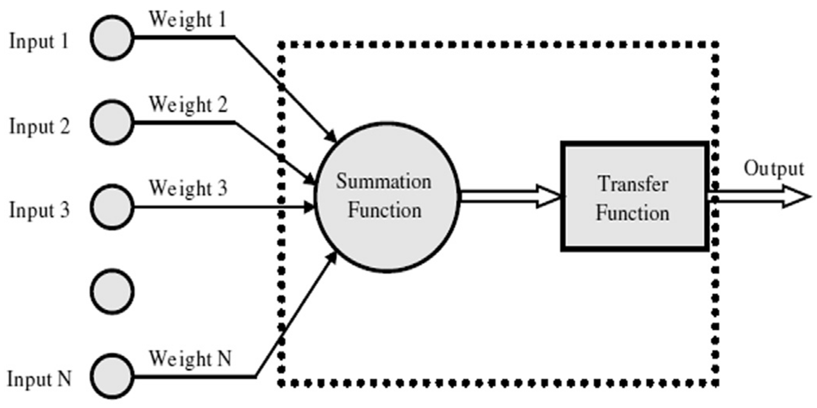
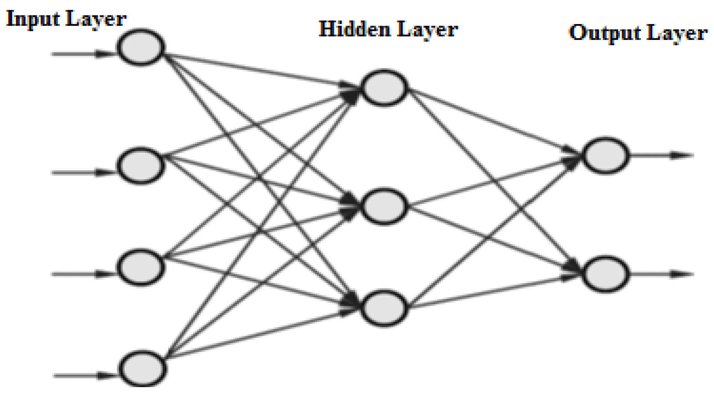
Figure 1 and
Figure 2 show an artificial neuron and a schematic of a multi-layer network, respectively. Each input is multiplied by a connection weight. A transfer function usually comprises linear or nonlinear algebraic equations.
3. Experimental Study
The details of the experimental study have been provided in the author’s previous paper [
25]. The current investigation is the continuation of the previous author’s study. The later was based on ANN models with 10 input parameters. Moreover, the former experimental database contained data collected over 1.5 years. In this current study, the new developed models are based on a larger database containing experimental data collected during two years.
The system mainly comprises mainly two flat-plate solar collectors, a thermally insulated vertical storage tank, a propane-fired tank as a source of auxiliary energy, and an air-handling unit. Solar radiation data was measured by two precision spectral pyranometers. One pyranometer was mounted on the collector frame at the same inclination and azimuth as the panels, and the second was mounted about a meter away from the panels on the horizontal building roof.
The experimental test matrix required data collection in the summer season with various weather conditions at different levels of solar irradiance. The experiments were conducted over a two-year period. A data logger with control capabilities is used to log data. The programme execution interval is 10 s to increase control accuracy and log more accurate summations of parameters. Data is logged every 1 min as an average or totalised value, as appropriate. Daily insolation, collector thermal efficiency, solar fraction, and energy consumed by the back-up storage tank were calculated.
The solar fraction (SF) is calculated by taking the amount of solar energy transferred to the heat exchanger (HX) divided by the sum of this value plus the energy content of fuel consumed by the auxiliary (Aux) storage tank burner. The thermal collector efficiency is calculated by taking the energy from heat transfer from the solar collector to the heat exchanger divided by the solar energy incident on the collector.
4. Development of ANN Models
This investigation undertook to examine the effects of input parameters on the ANN predictions of a solar energy system in Ottawa, Canada using the experimental data of input variables. The performance of the solar energy system is characterised by several design variables. The input variables were selected based on their effects on system performance. Selecting optimal inputs becomes a critical step prior to the model development itself. Computational cost can be substantially reduced but also can have a significant effect on the accuracy and robustness of the predictive model. In addition to drawing on the results from our previous ANN research [
25], the ANN simulation capabilities, as they responded to reduced input sets, were examined. The ultimate objective of this research was to verify whether equivalent performance predictions could be made as information was progressively removed from the inputs applied to the ANN models. If so, presumably this would allow predictions to be made without having to rely on certain sensors or sophisticated instrumentation. The ANN model parameters are shown in
Table 1.
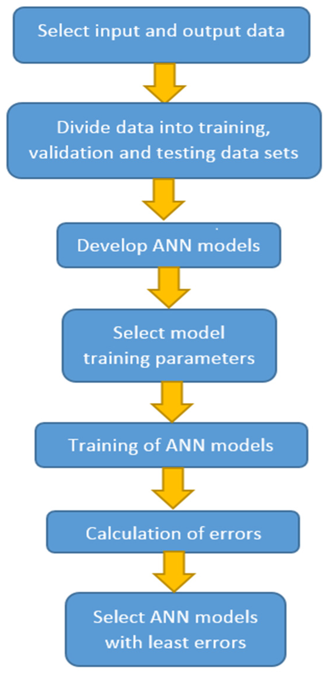
Figure 2 shows a simple diagram of the methodology for building an ANN model.
In case 1, represented by model 1, the ambient temperature (T
out) of the system was removed from the input matrix, creating a matrix of nine column vectors, as shown in
Table 1. Alternatively, case 2, represented by model 2, removed the solar radiation inputs for both the horizontal (G
h) and inclined (G
i) pyrometers, resulting in a matrix with eight total inputs. Finally, case 3 represented by model 3, was limited to seven total inputs, consisting only of the time of day and previous six solar tank temperatures (T
i, i = 1 to 6).
The neural network selected was a multilayer feed-forward perceptron (MLP) with one hidden layer, which is the most widely used network architecture for regression functions. The most popular training procedure for fully connected feed-forward networks is known as the supervised back-propagation learning scheme where the weights and biases are adjusted layer by layer from the output layer toward the input layer. The whole process of feeding forward with backward learning is then repeated until a satisfactory error level is reached or becomes stationary, as detailed in
Section 2 [
17,
20,
31,
32].
The data for the solar energy system comprised the influence of weather conditions for a given draw schedule in the summer season. The “Weather” parameter was assigned values of sunny, partly-cloudy, or cloudy.
The accuracy of the models is affected by the ratio of data used for training the model and data with which the model is validated and tested. In order to find the optimum ratio of training-validation-testing data in this work, the database is introduced to the model in three different ratios: 50%-25%-25%, 70%-15%-15% and 75%-12.5%-12.5%. It is found that the best ratios were the last two-cited. For convenience, of the data sets, 70% data patterns were used for training while the remaining 30% data patterns were randomly selected and used as validation (15%) and test data (15%) sets, respectively.
The data collected in the database are recorded by a data logger. The recorded data include the parameters of the solar energy system. Scenarios, each with a different set of test conditions, were created. Each day contained the experimental test data recorded at every minute of the day, resulting in 1440 data points per day. The input matrix contained inputs as listed in
Table 1. The data of each day used for a given case were placed one day after another, end to beginning, to make a matrix of
N by
n*1440 data values, where
N is the number of inputs and
n is the number of days used. These represent a significant amount of data patterns for the three data sets.
The back-propagation (BP) algorithm is the most popular and extensively used algorithm. As described in
Section 2, it consists of two phases: the feed forward pass and backward pass process. During the feed forward pass, the processing of information is propagated from the input layer to the output layer. In the backward pass, the difference between obtained network output value from the feed forward process and desired output is compared with the prescribed difference tolerance, and the error in the output layer is computed. This obtained error is propagated backwards to the input layer in order to update the connection. The BP training algorithm is a gradient descent algorithm. It tries to improve the performance of the network by minimising the total error, by changing the weights along its gradient. Training is halted when the testing set of sum squared errors (SSE) value stopped decreasing and started to increase, which is an indication of over training. In general, the prediction performances of the networks are evaluated using the SSE, the statistical coefficient of multiple determination or correlation coefficients (R
2) and mean relative error (MRE) values, which are calculated by the following expressions:
where
ai is the actual value,
pi is the ANN output or predicted value,
n is the number of output data.
The ANN Multi-Layer Perceptron (MLP)/Back-Propagation (BP) models were developed with three different learning algorithms: the Bayesian Regularisation (BR), the Levenberg–Marquardt (LM), and the Scaled Conjugate Gradient (SCG) algorithms. A variable number of neurons—16, 18, 20 and 22, were utilised in the hidden layer in order to express the output precisely. The training of the ANN models was stopped when the satisfactory level of error was attained. A total of twelve ANN models were built. The statistical measurements for model validation of various ANN models for the solar energy system are provided in
Table 2. It can be seen that the LM algorithm with 20 neurons in the hidden layer appeared to be the most optimal topology because the maximum correlation coefficient (R
2) and the low mean relative error (MRE) values were obtained.
The architectures of the two-layer back-propagation network with structures of 9, 8, and 7 inputs, 20 hidden neurons/layers, and 8 outputs were selected for the three ANN models of the solar energy system.
Finally, after founding the best parameters to use for this specific data set (
Figure 3), the simulations were run for the cases listed in
Table 1, and the results were saved for further analysis.
The neural network toolbox under MATLAB platform was applied for the ANN modelling [
33].
5. Results and Discussion
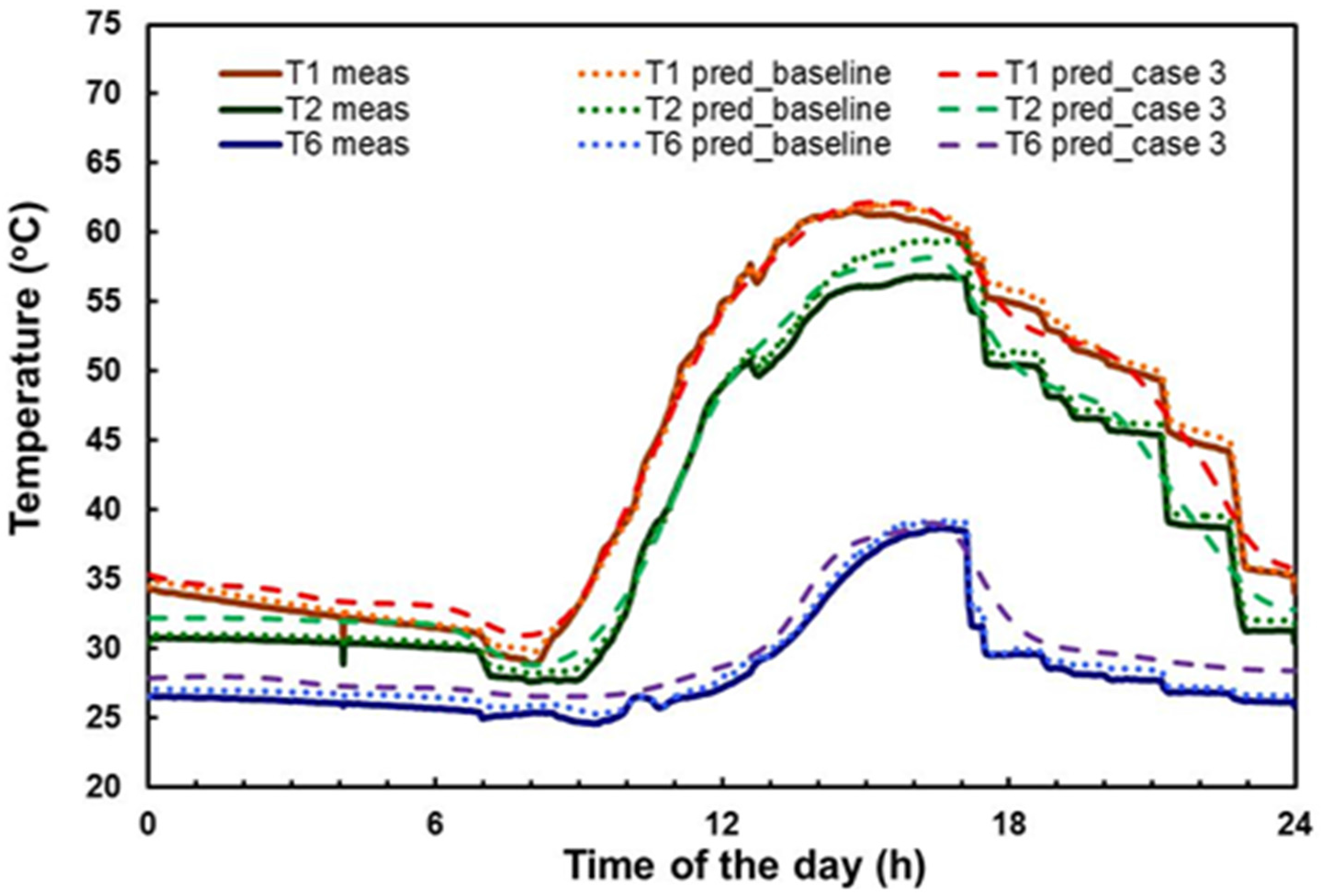
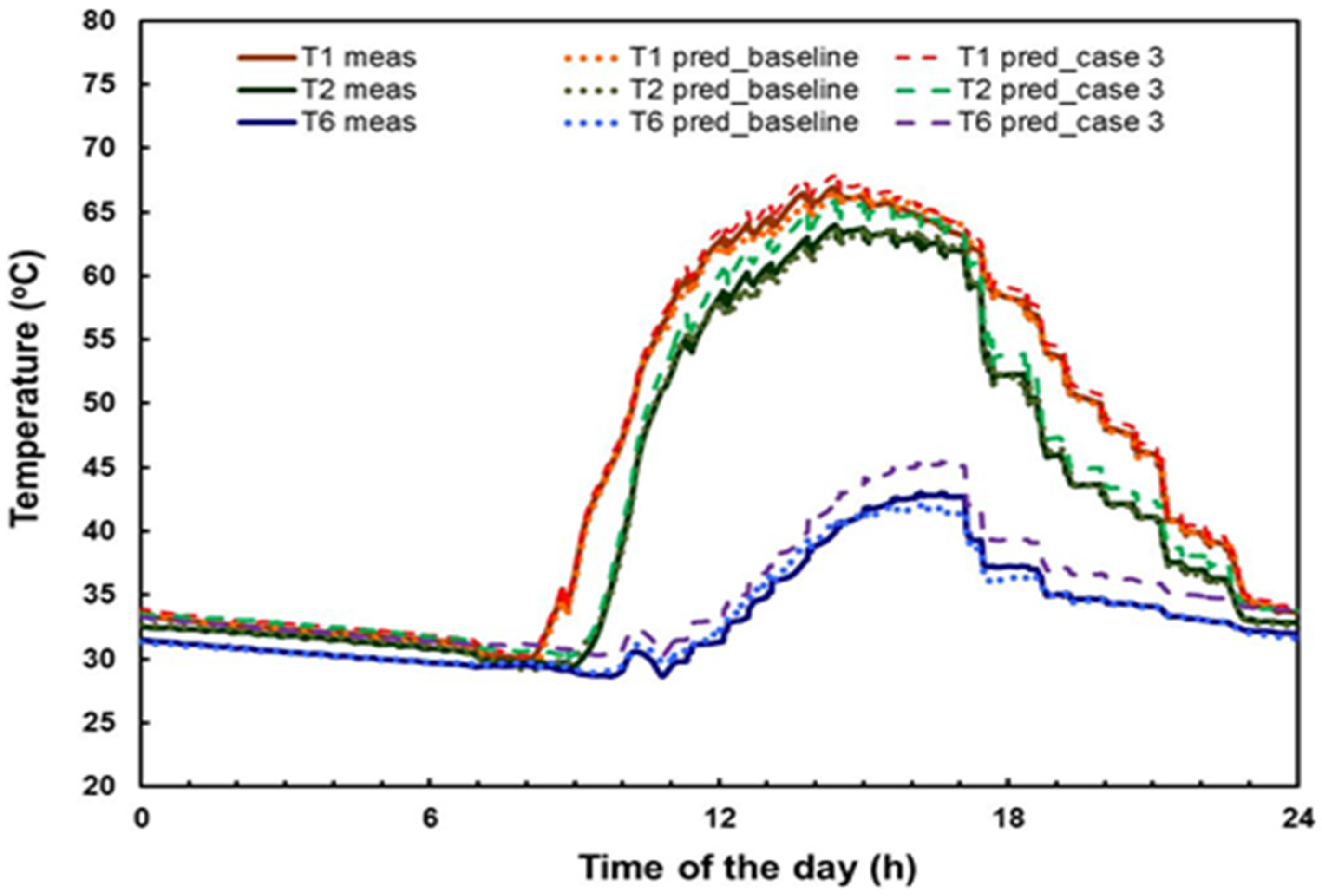
Figure 4 and
Figure 5 present a comparison between the measured and ANN–predicted solar tank temperatures T1–T6 as a function of time. The comparison is shown for the summer season and combined weather conditions for the testing data using the ANN models for 10 inputs (baseline case/baseline model) and 7 inputs (case 3/model 3), respectively. The figures shows that the predicted temperatures are very close to the experimental data, revealing a good agreement between the measured and ANN–predicted values for both cases.
Table 3 depicts a full assessment between the errors of ANN-predicted, preheat tank temperatures for the baseline and each of the three models with reduced input variables. The results correspond to the conditions mentioned above. It can be seen that, whilst the best predictions are obtained with the baseline model, the reduced input models for cases 1 and 2 (models 1 and 2) provide close values to the baseline result. The mean absolute and relative errors for the baseline model, models 1 and 2, are approximately 0.6 °C and 0.6%, respectively. The corresponding values for ANN model 3 are 1.3 °C and 4.3%, respectively. This discloses that, although the ANN predictions are satisfactory, the level of accuracy decreases for models with reduced inputs.
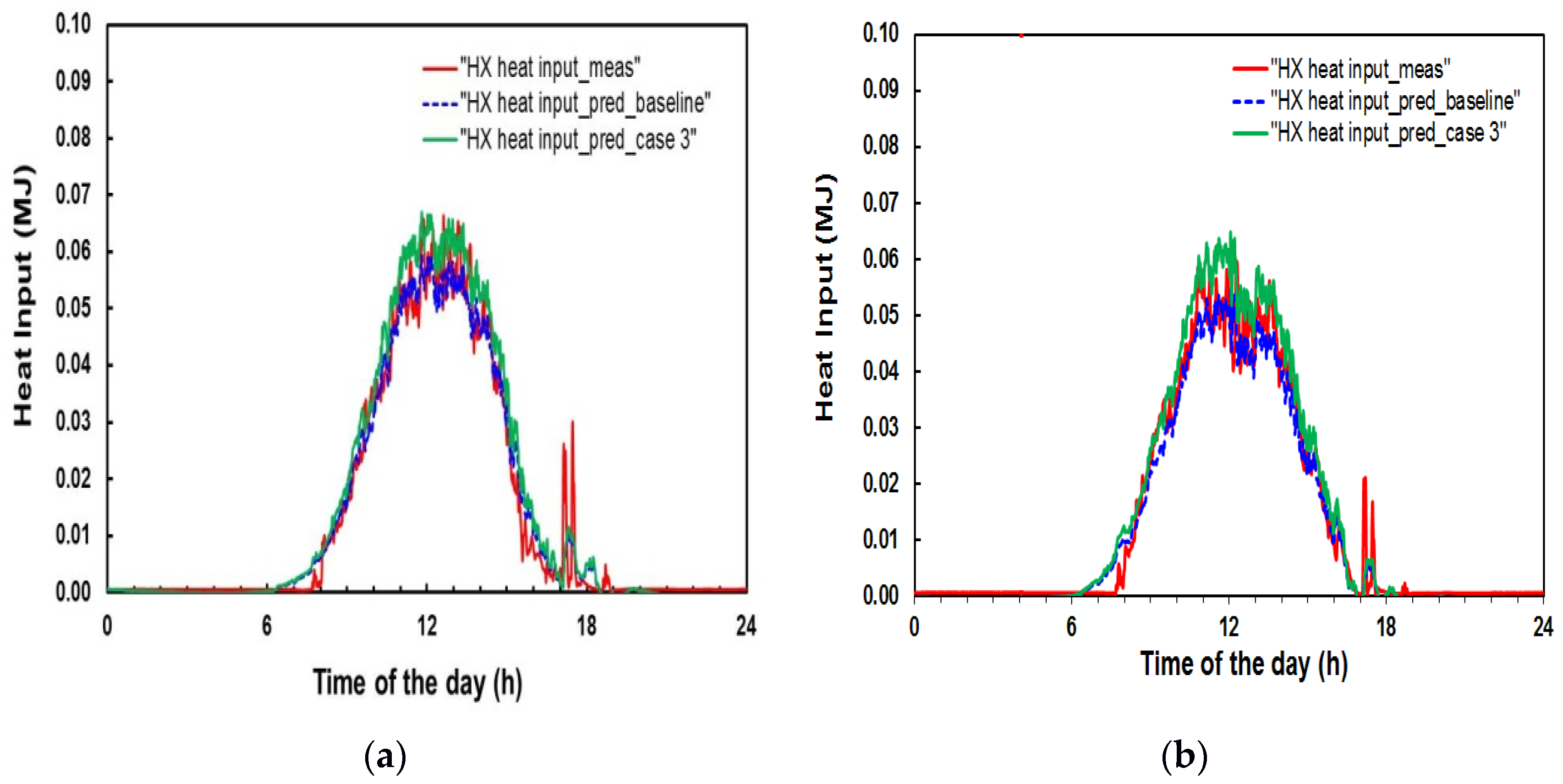
Figure 6a,b presents a comparison between the measured and ANN–predicted solar tank heat inputs as a function of time. The comparison is shown for the summer season and combined weather conditions for the training and testing data using the ANN models for 10 inputs (baseline case) and 7 inputs (case 3), respectively.
Figure 6a discloses that the simulated heat inputs based on the training model are very close to the experimental data, showing a good agreement between the measured and ANN–predicted values for both cases, while for the models using testing data, the agreement can be considered acceptable.
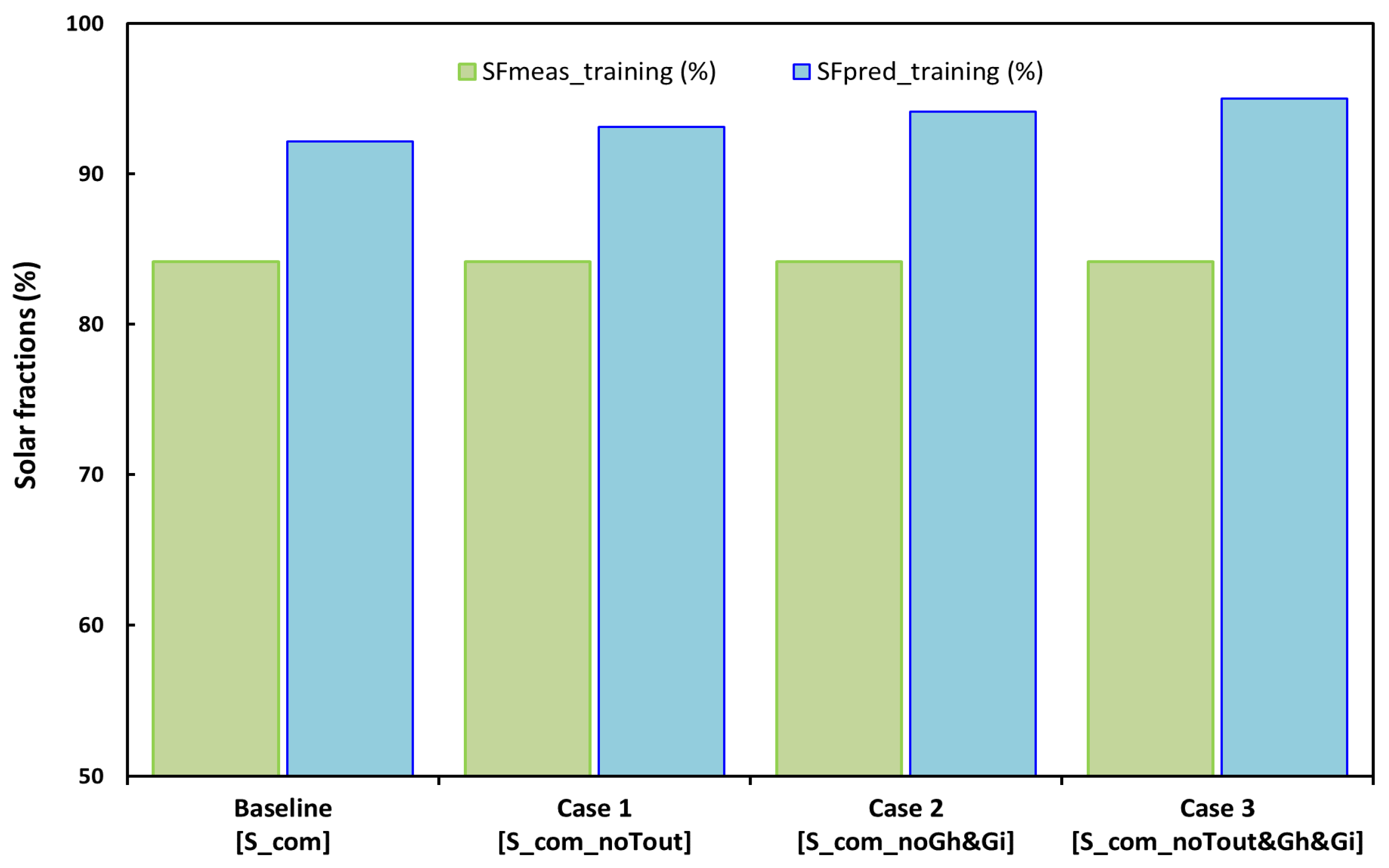
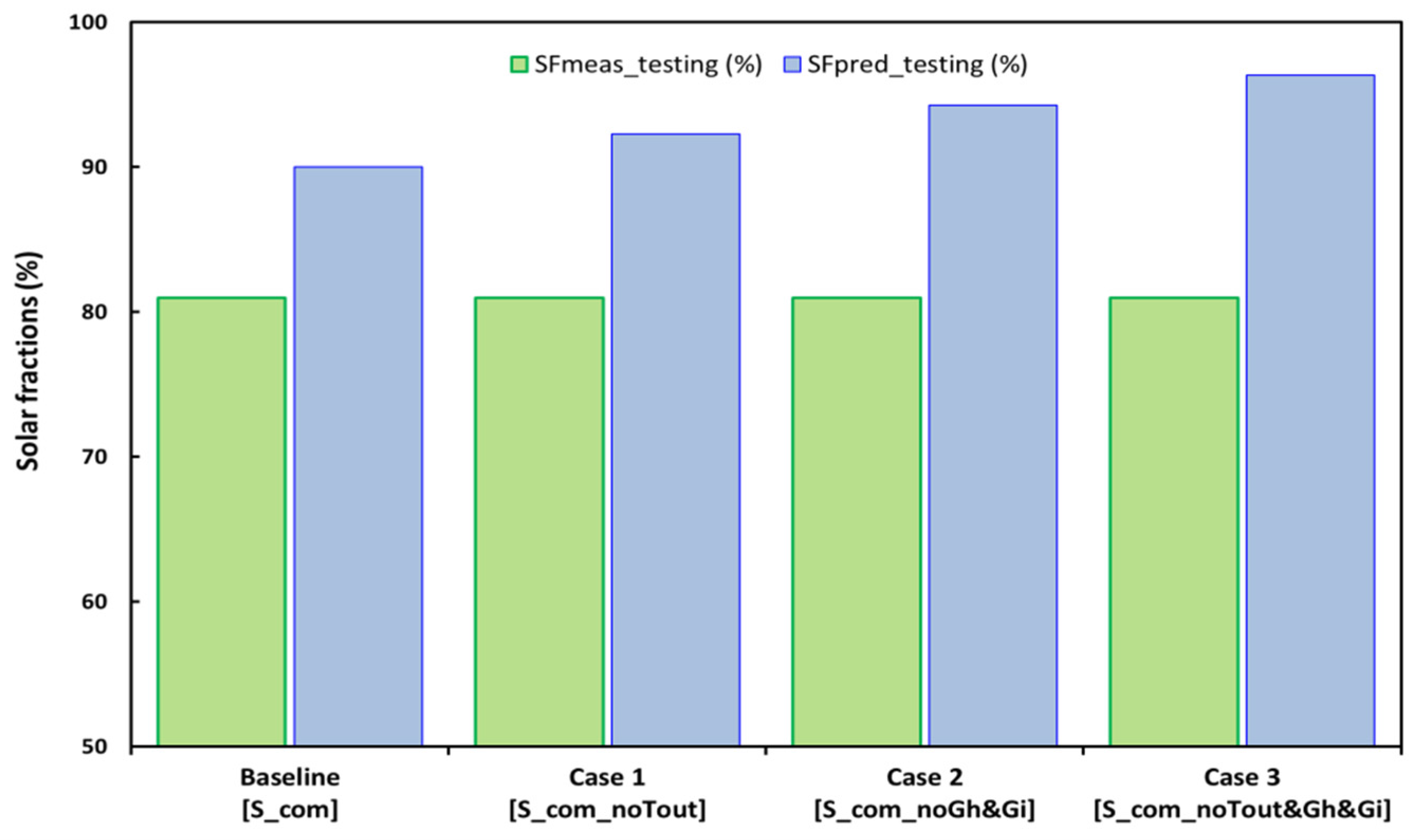
Table 4,
Figure 7 and
Figure 8 and
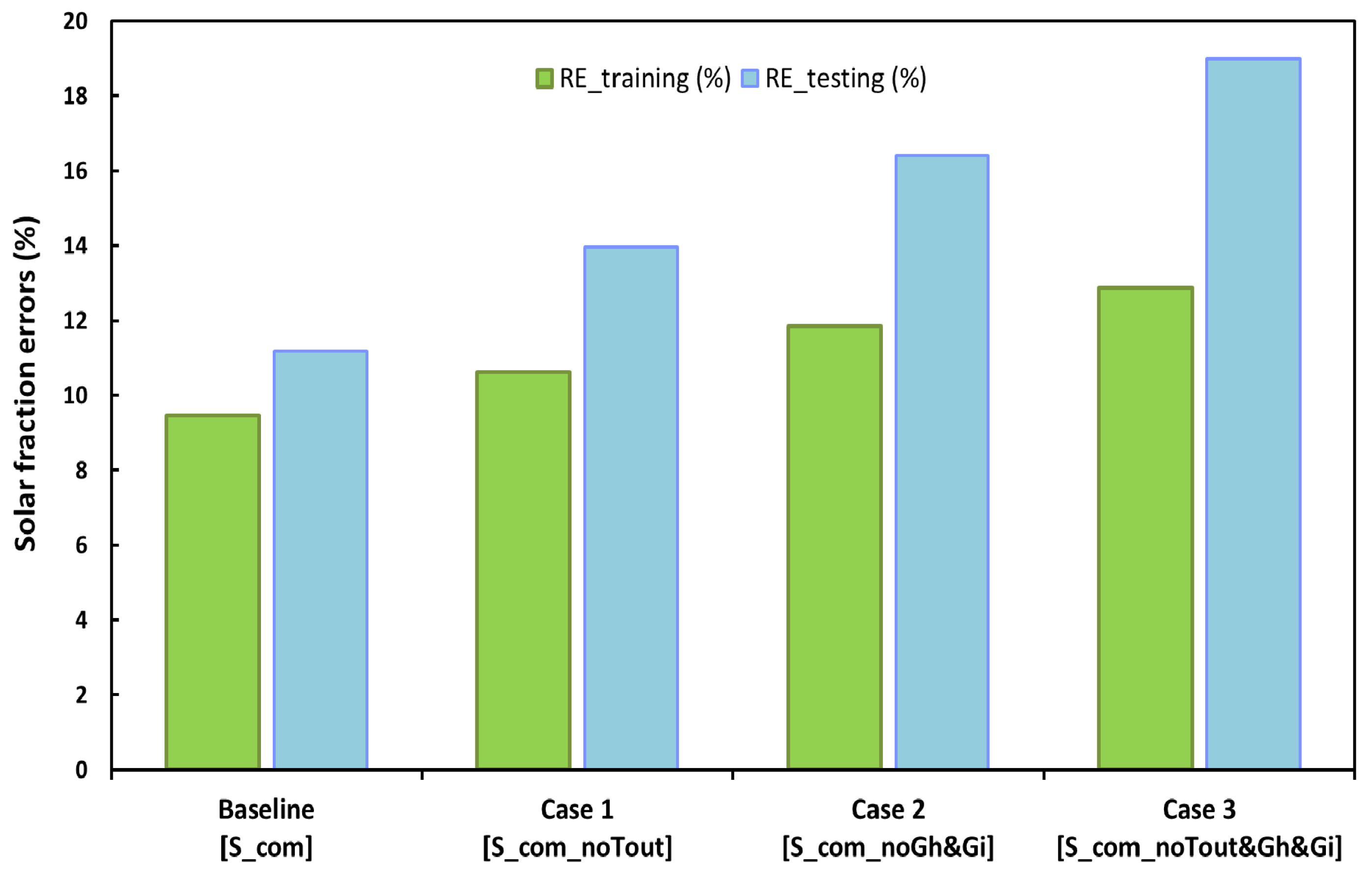
Figure 9 shows a detailed comparison between the results predicted by different ANN models and the measured solar fractions and errors for the training and testing data sets. As can be seen, the solar fractions are better predicted for the baseline case and case 1. Both the mean absolute errors (MAE) and the mean relative errors (MRE) increase for the models, with reduced inputs using testing data sets and scoring in the range of 9.0–15.4% and 11.2–19.0%, respectively. On the other hand, the mean absolute and relative errors for models using training data sets fall in the range of 8.0–10.8% and 9.5–12.9%, respectively.
These results demonstrate that, although the ANN solar fraction predictions are satisfactory for cases 1 and 2 across the full range of weather conditions, they can also be considered acceptable for case 3, wherein results were derived from a simplified ANN model using only the solar tank temperatures as input variables. Furthermore, as reported in [
24], it is assessed that the uncertainty in the measured solar fraction is in the range of 5–10%. Therefore, it must be concluded that this uncertainty biased the training process.
6. Conclusions
The influence of the number of input variables on the accuracy and robustness of the artificial neural network (ANN) model for predicting the performance parameters of an integrated solar energy system used for heating has been examined.
Three new ANN models with different input variables were developed and compared to a baseline ANN model previously developed by the authors. The back-propagation learning algorithm with three different variants, the Bayesian Regularisation (BR), the Levenberg–Marquardt (LM), and the Scaled Conjugate Gradient (SCG) algorithms, were applied in the network with 16, 18, 20, and 22 hidden neurons in order to find the optimal algorithm and topology of the ANN models with reduced input variables.
Comparison with experimental data from a solar energy system tested in Ottawa, Canada during two years under different weather conditions confirmed the good prediction accuracy attainable with each of the models using reduced input variables. However, it is likely right that the degree of model accuracy would gradually decrease with reduced inputs.
This investigation showed that the ANN method is a powerful tool for the performance prediction of energy systems with reduced input variables and limited experimental data.
The suitability of the modelling approach using ANNs as a practical engineering tool in renewable energy system performance analysis and prediction is clearly established.


