The Effect of Carbon Tax in Aviation Industry on the Multilateral Simulation Game

Abstract

With the end of the grace period (2016) of the aviation carbon tax (ACT) proposed by the EU, the EU is likely to restart the ACT. Hence, it becomes increasingly urgent to propose a feasible and effective scheme to restrict emissions in the aviation industry. We develop a two-stage game model to analyze three possible strategies (non-resistance, refusal of payment and ACT retaliation) in nine scenarios for three groups (the EU, developing countries and non-EU developed countries). The theoretical analyses and numerical simulations reveal that the EU will continue to impose the ACT. Simultaneously, imposing retaliatory ACT constitutes an ideal choice for non-EU developed countries. At present, refusing to pay the ACT is a practical strategy for developing countries; however, after the transitional phase, this group will tend to impose the ACT as developed countries by paying attention to increasing climate change. With optimal strategies for the above three groups, the ACT can be imposed effectively and efficiently by multilateral agreements within the framework of the market-based measure (MBM) scheme. This paper develops a game framework to simulate the ACT effect and to solve emission problems in the aviation industry by a multilateral perspective to achieve sustainability, which is of practical significance for nations and economies.

1. Introduction

The international aviation sector was included in the European Union Emissions Trading System (EU ETS) by the EU on 19 November 2008, which stipulates the payment of the aviation carbon tax (ACT) for all airlines flying over the EU airspace from 1 January 2012. However, the action had not attracted enough attention among nations and economies until 2012 when the measure was being implemented. In 2012, representatives from 32 countries held dialogues to boycott the forced payment of the ACT in Moscow. Due to the collective resistance and resolute refusal from all other nations, the EU’s tentative plan failed to progress as expected. At the beginning, the nature and feature of the ACT were discussed by researchers from the perspective of border tax [1,2], which leads to an increasing number of ACT-related research works about border tax adjustment [3,4,5]. Being regarded as a border tax, the ACT has been controversial in nature. From 2008 to the first half of 2013, the EU and other states had formed largely opposing positions, which led to a deadlock, that is the EU insisted on imposing the ACT, whilst other states all together resisted and refused to pay.

Since then, there has been a number of studies focusing on the ACT in the EU ETS. As the ACT has a wide influence, numerous papers analyze the impact of the ACT with interesting conclusions. From a macro perspective, the ACT may lead to an increase of costs for the global aviation industry [6], which will ultimately be transferred to consumers, with a greater impact on airlines in developing countries. However, by a dynamic simulation model named the energy-environment-economy model, including airlines in the EU ETS will reduce air transport ${\mathrm{CO}}_2$ emissions with small impacts on the aviation industry and macro economy [7]. Moreover, previous studies about including aviation emissions in the EU ETS have been reviewed [8]. At a national level, policy options are compared for aviation emission reduction in Korea by analyzing the economy with a system dynamics model [9], which indicates that the ETS is the most efficient approach. At a micro level, attention is mainly paid to competition and tourism. The impact of competition between EU airlines and other airlines around the world is analyzed using empirical estimations on three programs of EU ETS [10]. Afterwards, the influence on competition between the EU and non-EU airlines is continuously estimated from several aspects, including operational costs, fares, freight rate, etc. [11]. When it comes to tourism [12,13], the impact of emission reductions is estimated when levying the ACT on the tourism industry [14]. The number of visitors is also affected, as discussed in detail [15,16].

Given both the important and disputable nature of the ACT, related organizations have intervened since 2013, which dislocated the existing arrangements. The framework of multilateral negotiations under the International Civil Aviation Organization (ICAO) made some progress at the 38th ICAO Assembly held in September 2013. For the first time, the 38th ICAO Assembly designed a global aviation emission “roadmap” on 4 October 2013, which initiated a unified global aviation emission-related program named the market-based measure (MBM) in 2016, which is to be implemented from 2020. Research about implementing strategies of curbing aviation emissions mainly focuses on global schemes, measurements to reduce emissions and specific actions, while there have also been recent discussions about the MBM scheme [17,18]. Furthermore, some scholars focus on improving emission technology to achieve targets of emission reduction. For example, the global greenhouse gas problem can be solved by biofuels derived from waste oil [19]. The improved intensity index of greenhouse gas emission might solve the problems of the carbon border tax and the carbon trading system [20]. Other policies and projects are applied to curb emissions [21,22,23,24,25]. Besides the EU, a number of studies has investigated taking a series of measures on the ACT in other countries. The green tax matrix is raised to address green tax on aviation [26]. Both bilateral agreements and domestic actions are widely practiced to jointly seek ways to solve problems [27,28,29,30,31,32].

The literature related to the ACT is mainly concentrated into two methodologies, either qualified by the legality or quantified by game theory. Some studies use qualitative analysis of legal provisions to address the legitimacy of the ACT [33,34,35,36,37]. Additionally, pitfalls of the EU’s unilateral action are exposed, and laws signed by the U.S. to refuse the ACT are also discussed [38]. However, this is clarified to be reasonable, while the EU should convince other countries and prove that the extension of the EU ETS to the field of aviation is appropriate [39]. Other studies use game theory to analyze optimal strategies and possible policies of the ACT, where carbon taxation and emission trading are widely accepted and extensively discussed. According to the game, the best strategy is using the fuel tax and the ticket tax at the same time to reduce emissions [40]. Emission taxes and quotas are improved by considering asymmetric information about abatement costs [41]. A stochastic dynamic game is applied to consider possible tipping events [42], which solves the numerical equilibrium of carbon taxation and energy pricing strategies. By using dynamic Stackelberg games, joining the ${\mathrm{CO}}_2$ emission trading market is the strictly dominant strategy for various world organizations [43].

Despite the many important issues covered in existing studies about the ACT, a potential problem is that most of them have adopted a dual perspective, namely that of EU and non-EU countries. More specifically, four possible strategies are compared by using a two-stage game model [44], which indicates that the strategy of “refusal to pay” is the optimal strategy to obtain the highest welfare for China. In addition, the ACT game between EU and non-EU countries is analyzed by using the clever pig game model and dynamic game in the case of complete information [45]. In fact, the attitudes of developing countries and certain developed countries are changing. In regard to the resolution of the Assembly and the MBM scheme, the EU has responded positively with support. When it comes to developing countries, increasingly serious environmental problems raise the awareness and attention of some emerging economies. For instance. China has been accelerating the pace to protect the domestic and global environment, with seven provinces and cities as pilots for the establishment of the national ETS in 2017 [46]. However, the attitude of the U.S. is blurred, as President Donald Trump announced the U.S. withdrawal from the Paris Agreement for economic reasons on 1 June 2017. Since it is difficult for the international community to gain the upper hand in the game with the EU if the U.S. does not join, the attitude of the U.S. becomes critical. As a tripartite perspective is closer to reality and more appropriate in complex international situations, it would be preferable to have a new framework generalizing nations or economies into three groups: the EU, developing countries and non-EU developed countries. With the end of the grace period of the ACT, curbing aviation emissions through a variety of measures, including emissions trading and other policies, is critical and urgent for sustainability before 2020 [47]. To achieve sustainability, this paper develops a game framework to solve aviation emission problems from a complete tripartite perspective, which, in contrast to the dual perspective, may be more practical for nations and economies.

The remainder of the paper is organized as follows. Section 2 describes the game theoretic analytic framework including players, strategies, symbols, assumptions, analyses and scenarios. Section 3 is devoted to specific models and computes Nash equilibriums and optimal solutions, which analyzes nine scenarios by generalizing four models. Section 4 offers numerical simulations with a robust test. Concluding remarks are given in Section 5.

2. A Framework of Analytic Functions

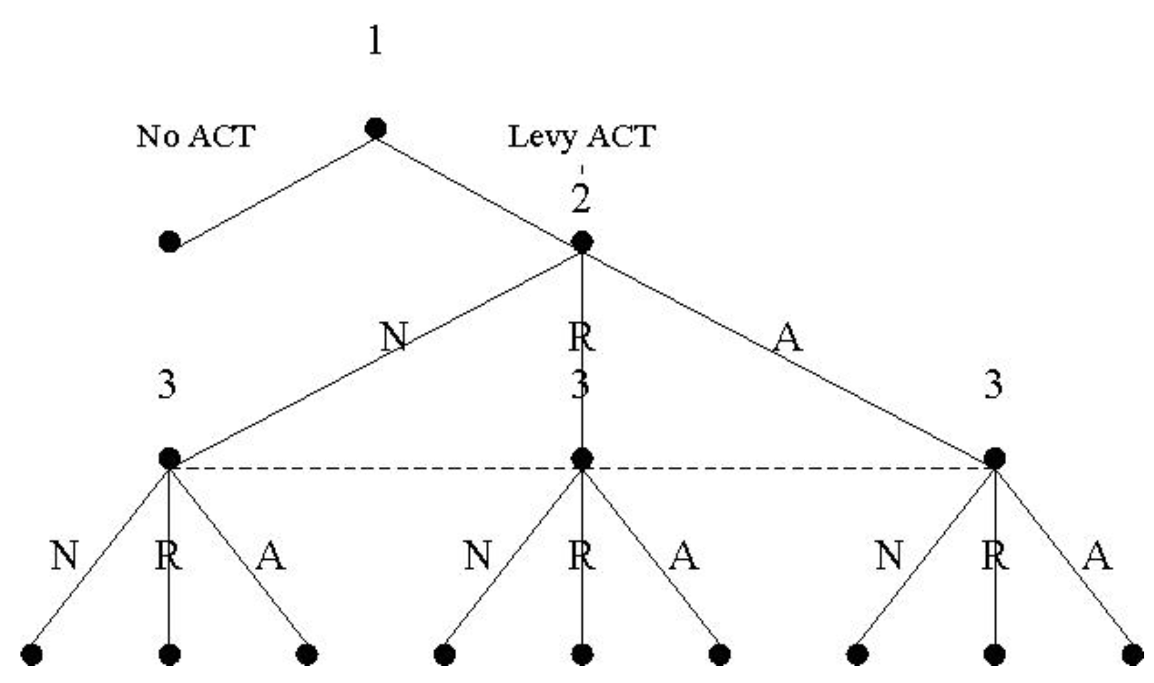
2.1. Players and Strategies

The ACT is a type of global game where countries are players and choose optimal strategies. Since the EU unilaterally proposed the aviation carbon tax, the roles of the parties in the game have changed as the proposal fell into abeyance. As some initial-refusal nations are more likely to be indecisive and may even suddenly defect to the EU, the dynamics have become even more volatile. In the past, there were only two sides, the EU and non-EU countries. At present, three groups of players can be identified: the challenger, which is the EU, the defender, as represented by China and other developing countries that are passively taking measures, and the meddler with hitchhiking and fuzzy attitudes, such as the U.S. and other important developed countries, except the EU.

After the EU proposed the ACT, three executable coping strategies from reality and research have been listed as follows for the other two players mentioned above:

Strategy 1, non-resistance: accepting to pay for the ACT while taking other measures to minimize loss. For instance, prioritize the Middle East, India or Russia when designing routes. Furthermore, developing countries can develop national clean development mechanism (CDM) projects to transfer the reduced carbon emissions into their own emission shares.

Strategy 2, refusal of payment: formulating legal provisions to prohibit domestic airlines from participating in the EU’s carbon trading scheme [43]; submitting a complaint or proposing litigation to relevant international organizations; maintaining the attitude of collective resistance and resolute refusal of the 2012 dialogues in Moscow to boycott the forced payment of the ACT [45].

Strategy 3 ACT retaliation: imposing similar ACT or other fees on airlines of EU members; imposing equal or higher tax rates; establishing carbon emission trading systems for EU airlines to buy carbon emission rights in other countries.

In the following three segments, we will discuss the impact on the aforementioned three groups following the EU proposal of the ACT. Additionally, the other two groups take one of the three possible strategies above in the game scenarios.

2.2. Symbols and Assumptions

Based on the analysis above, the three groups are: Challenger 1 (the EU), Defender 2 (developing countries) and Meddler 3 (other developed countries except the EU). Airline 1, Airline 2 and Airline 3, as players, represent airlines of the three groups, respectively. To focus our research on appropriate strategies and optimal tax rates of the groups, aviation carbon emissions within domestic lines are ignored in the models, and we only consider international lines involving Challenger 1, Defender 2 and Meddler 3.

We assume that the quantity of aviation carbon emissions on airlines from Challenger 1 to Defender 2 is $q_{12}$, and the quantity on airlines from Challenger 1 to Meddler 3 is $q_{13}$; apparently, $q_{12}>0$, $q_{13}>0$. Similarly, the quantity of aviation carbon emissions on airlines from Defender 2 to Challenger 1 and Meddler 3 are $q_{21}$, $q_{23}$, respectively, and airlines from Meddler 3 to Challenger 1 and Defender 2 are $q_{31}$, $q_{32}$, respectively, where $q_{ij}>0(i=1,2,3,j=1,2,3)$. Hence, the quantity of total emissions is $Q=q_{12}+q_{13}+q_{21}+q_{23}+q_{31}+q_{32}$.

We assume that Challenger 1 (the EU) imposes the ACT, rate t, on airlines of all nations and economies. According to the analysis of ACT retaliation in Section 3.1, both Defender 2 and Meddler 3 are likely to impose the aviation carbon tax for retaliation. Tax rates of Defender 2 and Meddler 3 are assumed to be $\theta t$ and $\xi t$, respectively, where $\theta >0$, $\xi >0$.

In these models, although the costs of aviation operation, ticket prices, passengers’ attendance and other factors are not considered to affect the profits of airlines, adding these factors will not change the results and conclusions of the models. Firstly, the profits of airlines proportionally increases with the total mileage and emissions; secondly, as the tax is ultimately transferred to consumers, the consumers may choose alternative means of transport if an excessive quantity of emissions causes high tax burden, which will lead to a fall in the number of passengers, operating times and the airline companies’ revenues. Therefore, the profit of airlines can be assumed as a quadratic function involved in aviation emissions. Let B denote the profit function by [48].

$$B\left(Q\right)=a{\left(Q\right)}^2+b\left(Q\right)$$

(1)

$B\left(Q\right)$ is a monotonically-increasing concave function of Q, where $a<0$, $b>0$; the first derivative of the function is greater than zero, and the second derivative is less than zero, which indicate that the profit increases with the increase of emissions, while the growth speed first increases and then decreases.

The profit function $B_i$ of airline i is the share in the function B Equations (2)–(4).

$$\begin{array}{c}{B}_1=B_{12}+B_{13}\hfill \\ =\frac{q_{12}}{q_{12}+q_{21}}[a{(q_{12}+q_{21})}^2+b(q_{12}+q_{21})]+\frac{q_{13}}{q_{13}+q_{31}}[a{(q_{13}+q_{31})}^2+b(q_{13}+q_{31})]\hfill \\ =[a{\left(q_{12}\right)}^2+a·q_{12}{q}_{21}+b·q_{12}]+[a{\left(q_{13}\right)}^2+a·q_{13}{q}_{31}+b·q_{13}]\hfill \end{array}$$

(2)

$$\begin{array}{c}{B}_2=B_{21}+B_{23}\hfill \\ =\frac{q_{21}}{q_{21}+q_{12}}[a{(q_{21}+q_{12})}^2+b(q_{21}+q_{12})]+\frac{q_{23}}{q_{23}+q_{32}}[a{(q_{23}+q_{32})}^2+b(q_{23}+q_{32})]\hfill \\ =[a{\left(q_{21}\right)}^2+a·q_{12}{q}_{21}+b·q_{21}]+[a{\left(q_{23}\right)}^2+a·q_{23}{q}_{32}+b·q_{23}]\hfill \end{array}$$

(3)

$$\begin{array}{c}{B}_3=B_{32}+B_{31}\hfill \\ =\frac{q_{32}}{q_{32}+q_{31}}[a{(q_{32}+q_{23})}^2+b(q_{32}+q_{23})]+\frac{q_{31}}{q_{13}+q_{31}}[a{(q_{13}+q_{31})}^2+b(q_{13}+q_{31})]\hfill \\ =[a{\left(q_{32}\right)}^2+a·q_{32}{q}_{23}+b·q_{32}]+[a{\left(q_{31}\right)}^2+a·q_{13}{q}_{31}+b·q_{31}]\hfill \end{array}$$

(4)

The damage function caused by carbon dioxide emissions can be assumed as Equation (5), where parameter ${\gamma }_i>0$, representing the attention to climate change in different countries by [4]. The greater attention countries pay to climate change, the greater the parameter ${\gamma }_i$ is.

$$D_i=\frac{{\gamma }_i·[{{\displaystyle \sum _{j\ne i}}(q_{ij}+q_{ji})}^2]}{2},(i,j=1,2,3)$$

(5)

In addition, we apply the revenue function to balance the financial performance, involving the profit function of the mileage and the damage function of the emissions, and the environmental performance represented by parameter $C_i$ to achieve sustainability. More specifically, $C_i$ is introduced to describe the tacit cost of airlines including the R&D input in energy savings and emission reduction, other expenditure on the development of sustainable technologies or corporate social responsibility, etc. The revenue function of countries is represented by ${\psi }_i$, and the revenue function of airlines is represented by ${\pi }_i$.

In this paper, symbols in subscript imply players, and symbols in superscript are relevant to the number of scenarios.

2.3. Analyses and Scenarios

In this section, the issue of ACT is discussed by using two-stage game models for three groups, with the six players being Challenger 1 (the EU), Defender 2 (developing countries), Meddler 3 (non-EU developed countries) and their airlines. The game is divided into two stages:

Stage 1: Following the unilateral proposal of the ACT (rate t) by Challenger 1 (the EU), Defender 2 and Meddler 3, at the same time, pick one out of the following three strategies.

Strategy 1 non-resistance: accepting to pay for the ACT and making concessions;

Strategy 2 refusal of payment: refusing to pay without further sanctions against each other;

Strategy 3 ACT retaliation: imposing similar ACT on all countries at an appropriate rate.

As Defender 2 and Meddler 3 take actions separately, the game evolves into the following nine scenarios on the basis of the three strategies above:

Scenario 1: Both Defender 2 and Meddler 3 adopt refusal of payment;

Scenario 2: Defender 2 adopts refusal of payment; meddler imposes ACT retaliation;

Scenario 3: Defender 2 imposes ACT retaliation; Meddler 3 adopts refusal of payment;

Scenario 4: Both Defender 2 and Meddler 3 impose ACT retaliation;

Scenario 5: Both Defender 2 and Meddler 3 choose non-resistance;

Scenario 6: Defender 2 chooses non-resistance; Meddler 3 adopts refusal of payment;

Scenario 7: Defender 2 chooses non-resistance; Meddler 3 imposes ACT retaliation;

Scenario 8: Defender 2 adopts refusal of payment; Meddler 3 chooses non-resistance;

Scenario 9: Defender 2 imposes ACT retaliation; Meddler 3 chooses non-resistance.

Figure 1 shows Stage 1 of the game in extended expression (omitting the corresponding payoff of players), where the three groups in the game are represented by 1, 2, 3, with strategies non-resistance (N for short), refusal of payment (R for short) and ACT retaliation (A for short):

Stage 2: After observing rate t and possible retaliatory ACT rate $\theta t$ or $\xi t$, Airlines 1, 2 and 3 determine the carbon dioxide emissions $q_{12},q_{13},q_{21},q_{23},q_{31}$ and $q_{32}$ at the same time.

However, the premise for imposing retaliatory ACT is to pay for the ACT (non-resistance) of other groups out of fairness. Strategy non-resistance is equal to strategy ACT retaliation when the tax rate of ACT is zero.

Therefore, Scenario 6 (N, R) is the special circumstance of Scenario 3 (A, R) when the retaliatory ratio $\theta$ of Defender 2 is zero. Similarly, Scenario 8 (R, N) is the special circumstance of Scenario 2 (R, A) when the retaliatory ratio $\xi$ of Meddler 3 is zero. Moreover, Scenario 5 (N, N), Scenario 7 (N, A) and Scenario 9 (A, N) are special circumstances of Scenario 4 (A, A).

After incorporating strategy N into strategy A when the tax rate is zero, there are only four scenarios (R, R), (R, A), (A, R), (A, A) left, all of which are composed of strategy R and strategy A. We will conduct further analyses and provide mathematical proofs.

According to different strategies taken by Defender 2 and Meddler 3, we build four models for the nine scenarios above and solve Nash equilibriums as follows:

Model 1 (R, R): refusal of payment for both;

Model 2 (R, A): Defender 2 refusal of payment, Meddler 3 ACT retaliation;

Model 3 (A, R): Defender 2 ACT retaliation, Meddler 3 refusal of payment;

Model 4 (A, A): ACT retaliation for both.

3. Two-Stage Game Models and Nash Equilibriums

3.1. Model 1: (R, R)

Stage 1: Challenger 1 decides to impose ACT with optimal rate t; then, both Defender 2 and Meddler 3 adopt refusal of payment. Stage 2: Airline 1 of Challenger 1 decides on $q_{12}$ and $q_{13}$ after observing rate t; similarly, Airline 2 of Defender 2 decides on $q_{21}$ and $q_{23}$ and Airline 3 of Meddler 3 on $q_{31}$ and $q_{32}$.

The revenue functions of Challenger 1, Airline 1, Defender 2, Airline 2, Meddle 3 and Airline 3 are given by:

$$\begin{array}{c}{\psi }_1^1={\pi }_1^1+t(q_{12}+q_{13})-\frac{{\gamma }_1[{(q_{12}+q_{21})}^2+{(q_{13}+q_{31})}^2]}{2}\hfill \\ {\pi }_1^1=[a{\left(q_{12}\right)}^2+a{q}_{12}{q}_{21}+b{q}_{12}-t{q}_{12}]+[a{\left(q_{13}\right)}^2+a{q}_{13}{q}_{31}+b{q}_{13}-t{q}_{13}]-C_1\hfill \\ {\psi }_2^1={\pi }_2^1-\frac{{\gamma }_2[{(q_{12}+q_{21})}^2+{(q_{23}+q_{32})}^2]}{2}\hfill \\ {\pi }_2^1=[a{\left(q_{21}\right)}^2+a{q}_{12}{q}_{21}+b{q}_{21}]+[a{\left(q_{23}\right)}^2+a{q}_{23}{q}_{32}+b{q}_{23}]-C_2\hfill \\ {\psi }_3^1={\pi }_3^5-\frac{{\gamma }_3[{(q_{13}+q_{31})}^2+{(q_{23}+q_{32})}^2]}{2}\hfill \\ {\pi }_3^1=[a{\left(q_{32}\right)}^2+a{q}_{32}{q}_{23}+b{q}_{32}]+[a{\left(q_{31}\right)}^2+a{q}_{13}{q}_{31}+b{q}_{31}]-C_3\hfill \end{array}$$

(6)

By maximizing the revenue functions of airlines in Stage 2, we solve equilibriums on carbon dioxide emissions of Airline 1, 2 and 3 based on Equation (6).

$$\begin{array}{c}{q}_{12}^1=\frac{2t-b}{3a},q_{21}^1=\frac{-t-b}{3a},q_{13}^1=\frac{2t-b}{3a},q_{31}^1=\frac{-t-b}{3a},q_{23}^1=q_{32}^1=-\frac{b}{3a}\hfill \end{array}$$

(7)

According to the first-order condition of Challenger 1 revenue function $\frac{\partial {\psi }_1^1}{\partial t}=0$, Equation (7) is substituted into Equation (6) to obtain the optimal tax rate under Nash equilibrium.

$$\begin{array}{c}{t}^1=-\frac{ab+2b{\gamma }_1}{4a-{\gamma }_1}\hfill \end{array}$$

(8)

The total quantity of carbon dioxide emissions is given by:

$$\begin{array}{c}{Q}^1=q_{12}^1+q_{21}^1+q_{13}^1+q_{31}^1+q_{23}^1+q_{32}^1=-\frac{6b}{4a-{\gamma }_1}-\frac{2b}{3a}\hfill \end{array}$$

(9)

The revenues of airlines and countries can be obtained under the equilibrium by substituting Equations (7) and (8).

The revenues of airlines and countries under the equilibrium are as follows:

$$\begin{array}{c}{\pi }_1^1=-\frac{2b^2{(2a+{\gamma }_1)}^2}{a{(4a-{\gamma }_1)}^2}-C_1\hfill \end{array}$$

(10)

$$\begin{array}{c}{\psi }_1^1=-\frac{b^2(a+2{\gamma }_1)}{a(4a-{\gamma }_1)}-C_1\hfill \end{array}$$

(11)

$$\begin{array}{c}{\pi }_2^1=-\frac{b^2(25a^2-26a{\gamma }_1+10{{\gamma }_1}^2)}{9a{(4a-{\gamma }_1)}^2}-C_2\hfill \end{array}$$

(12)

$$\begin{array}{c}{\psi }_2^1=-\frac{b^2(50a^3-52a^2{\gamma }_1+145a^2{\gamma }_2+20a{{\gamma }_1}^2-32a{\gamma }_1{\gamma }_2+4{{\gamma }_1}^2{\gamma }_2)}{18a^2{(4a-{\gamma }_1)}^2}-C_2\hfill \end{array}$$

(13)

$$\begin{array}{c}{\pi }_3^1=-\frac{b^2(25a^2-26a{\gamma }_1+10{{\gamma }_1}^2)}{9a{(4a-{\gamma }_1)}^2}-C_3\hfill \end{array}$$

(14)

$$\begin{array}{c}{\psi }_3^1=-\frac{b^2(50a^3-52a^2{\gamma }_1+145a^2{\gamma }_3+20a{{\gamma }_1}^2-32a{\gamma }_1{\gamma }_3+4{{\gamma }_1}^2{\gamma }_3)}{18a^2{(4a-{\gamma }_1)}^2}-C_3\hfill \end{array}$$

(15)

3.2. Model 2: (R, A)

Stage 1: Challenger 1 decides to impose ACT; then, Defender 2 adopts refusal of payment, and Meddler 3 imposes ACT retaliation, rate $\xi t$. In this stage, Challenger 1 considers $\xi t$ when setting optimal rate t. Stage 2: Airline 1 of Challenger 1 decides on $q_{12}$ and $q_{13}$ after observing rate t and rate $\xi t$; similarly, Airline 2 of Defender 2 decides on $q_{21}$ and $q_{23}$ and Airline 3 of Meddler 3 on $q_{31}$ and $q_{32}$.

The revenue functions of Challenger 1, Airline 1, Defender 2, Airline 2, Meddle 3 and Airline 3 are given by:

$$\begin{array}{c}{\psi }_1^2={\pi }_1^2+t(q_{12}+q_{31}+q_{13})-\frac{{\gamma }_1[{(q_{12}+q_{21})}^2+{(q_{13}+q_{31})}^2]}{2}\hfill \\ {\pi }_1^2=[a{\left(q_{12}\right)}^2+a{q}_{12}{q}_{21}+b{q}_{12}-t{q}_{12}]+[a{\left(q_{13}\right)}^2+a{q}_{13}{q}_{31}+b{q}_{13}-t{q}_{13}-\xi t{q}_{13}]-C_1\hfill \\ {\psi }_2^2={\pi }_2^2-\frac{{\gamma }_2[{(q_{12}+q_{21})}^2+{(q_{23}+q_{32})}^2]}{2}\hfill \\ {\pi }_2^2=[a{\left(q_{21}\right)}^2+a{q}_{12}{q}_{21}+b{q}_{21}]+[a{\left(q_{23}\right)}^2+a{q}_{23}{q}_{32}+b{q}_{23}]-C_2\hfill \\ {\psi }_3^2={\pi }_3^2+\xi t·(q_{13}+q_{31}+q_{32})-\frac{{\gamma }_3[{(q_{13}+q_{31})}^2+{(q_{23}+q_{32})}^2]}{2}\hfill \\ {\pi }_3^2=[a{\left(q_{32}\right)}^2+a{q}_{32}{q}_{23}+b{q}_{32}-\xi t{q}_{32}]+[a{\left(q_{31}\right)}^2+a{q}_{13}{q}_{31}+b{q}_{31}-t{q}_{31}-\xi t{q}_{31}]-C_3\hfill \end{array}$$

(16)

Then, we solve equilibriums on the carbon dioxide emissions of Airline 1, 2 and 3 by maximizing the revenue functions of airlines in Stage 2 for Scenario 2 (R, A).

$$\begin{array}{c}{q}_{12}^2=\frac{2t-b}{3a},q_{21}^2=\frac{-t-b}{3a},q_{13}^2=\frac{t-b+2t\xi }{3a},q_{31}^2=\frac{t-b-t\xi }{3a},q_{32}^2=\frac{2\xi t-b}{3a},q_{23}^2=\frac{-\xi t-b}{3a}\hfill \end{array}$$

(17)

We substitute q above in the first-order condition of Challenger 1 to obtain the optimal tax rate under Nash equilibrium.

$$t^2=\frac{6b{\gamma }_1-3ab+4ab\xi +2b{\gamma }_1\xi }{5{\gamma }_1-14a+2a\xi +4{\gamma }_1\xi +8a{\xi }^2+{\gamma }_1{\xi }^2}$$

(18)

The total quantity of carbon dioxide emissions in Model 2 is given by:

$$\begin{array}{c}{Q}^2=q_{12}^2+q_{21}^2+q_{13}^2+q_{31}^2+q_{23}^2+q_{32}^2=-\frac{b(2{\gamma }_1{\xi }^2+6{\gamma }_1\xi +12{\gamma }_1)+ab(40{\xi }^2+6\xi -75)}{3a(5{\gamma }_1-14a+2a\xi +4{\gamma }_1\xi +8a{\xi }^2+{\gamma }_1{\xi }^2)}\hfill \end{array}$$

(19)

We obtain equilibrium q and t in Scenario 8 (R, N) with $\xi =0$.

The revenue of Airline 1 under the equilibrium is given by:

$$\begin{array}{c}{\pi }_1^2=-\frac{b^2}{9a}·\frac{C^{2\left(3\right)}+D^2}{{(A^{2\left(3\right)}+B^2)}^2}-C_1\hfill \end{array}$$

(20)

where:

$$\begin{array}{c}{A}^{2\left(3\right)}=5{\gamma }_1-14a\hfill \\ B^2=2a\xi +4\xi {\gamma }_1+8a{\xi }^2+{\xi }^2{\gamma }_1\hfill \\ C^{2\left(3\right)}=185a^2+134a{\gamma }_1+50{{\gamma }_1}^2\hfill \\ D^2=10{\xi }^4{{\gamma }_1}^2+60{\xi }^3{{\gamma }_1}^2+92{\xi }^2{{\gamma }_1}^2+20\xi {{\gamma }_1}^2\hfill \\ +a(16{\gamma }_1{\xi }^4-36{\gamma }_1{\xi }^3-142{\gamma }_1{\xi }^2+296{\gamma }_1\xi )\hfill \\ +a^2(64{\xi }^4-96{\xi }^3-76{\xi }^2+8\xi )\hfill \end{array}$$

(21)

The revenue of Country 1 under the equilibrium is given by:

$$\begin{array}{c}{\psi }_1^2=-\frac{b^2}{18a^2}·\frac{E^{2\left(3\right)}+F^2}{A^{2\left(3\right)}+B^2}-C_1\hfill \end{array}$$

(22)

where:

$$\begin{array}{c}{E}^{2\left(3\right)}=-65a^2-56a{\gamma }_1+4{{\gamma }_1}^2\hfill \\ F^2=4{\xi }^2{{\gamma }_1}^2+8\xi {{\gamma }_1}^2+a^2(16{\xi }^2+32\xi )-a(52{\gamma }_1{\xi }^2-4{\gamma }_1\xi )\hfill \end{array}$$

(23)

The revenue of Airline 2 under the equilibrium is given by:

$$\begin{array}{c}{\pi }_2^2=-\frac{b^2}{9a}·\frac{G^{2\left(3\right)}+H^2}{{(A^{2\left(3\right)}+B^2)}^2}-C_2\hfill \end{array}$$

(24)

where:

$$\begin{array}{c}{G}^{2\left(3\right)}=485a^2-514a{\gamma }_1+146{{\gamma }_1}^2\hfill \\ H^2=-8{\xi }^4{{\gamma }_1}^2-42{\xi }^3{{\gamma }_1}^2-22{\xi }^2{{\gamma }_1}^2\hfill \\ +a(-20{\gamma }_1{\xi }^4+39{\gamma }_1{\xi }^3+362{\gamma }_1{\xi }^2-65{\gamma }_1\xi )\hfill \\ +142\xi {{\gamma }_1}^2+a^2(64{\xi }^4+192{\xi }^3-412{\xi }^2-302\xi )\hfill \end{array}$$

(25)

The revenue of Country 2 under the equilibrium is given by:

$$\begin{array}{c}{\psi }_2^2=-\frac{b^2}{18a^2}·\frac{I^2+J^2}{{(A^{2\left(3\right)}+B^2)}^2}-C_2\hfill \end{array}$$

(26)

where:

$$\begin{array}{c}{I}^2=970a^3-1028a^2{\gamma }_1+1409a^2{\gamma }_2+292a{{\gamma }_1}^2-760a{\gamma }_1{\gamma }_2+116{{\gamma }_1}^2{\gamma }_2\hfill \\ J^2=4{\gamma }_2{\xi }^4{{\gamma }_1}^2+24{\gamma }_2{\xi }^3{{\gamma }_1}^2+56{\gamma }_2{\xi }^2{{\gamma }_1}^2+88{\gamma }_2\xi {{\gamma }_1}^2+a(-16{\xi }^4{{\gamma }_1}^2-84{\xi }^3{{\gamma }_1}^2)\hfill \\ +a(-44{\xi }^2{{\gamma }_1}^2+284\xi {{\gamma }_1}^2+64{\gamma }_2{\xi }^4{\gamma }_1+240{\gamma }_2{\xi }^3{\gamma }_1+296{\gamma }_2{\xi }^2{\gamma }_1-272{\gamma }_2\xi {\gamma }_1)\hfill \\ +a^2(724{\xi }^2{\gamma }_1-1423{\xi }^2{\gamma }_2+78{\xi }^3{\gamma }_1+168{\xi }^3{\gamma }_2-40{\xi }^4{\gamma }_1+400{\xi }^4{\gamma }_2)\hfill \\ +a^2(-130\xi {\gamma }_1-392\xi {\gamma }_2)+a^3(128{\xi }^4+384{\xi }^3-824{\xi }^2-604\xi )\hfill \end{array}$$

(27)

The revenue of Airline 3 under the equilibrium is given by:

$$\begin{array}{c}{\pi }_3^2=-\frac{b^2}{9a}·\frac{K^{2\left(3\right)}+L^2}{{(A^{2\left(3\right)}+B^2)}^2}-C_3\hfill \end{array}$$

(28)

where:

$$\begin{array}{c}{K}^{2\left(3\right)}=317a^2-118a{\gamma }_1+26{{\gamma }_1}^2\hfill \\ L^2=-18{\xi }^4{{\gamma }_1}^2-108{\xi }^3{{\gamma }_1}^2-160{\xi }^2{{\gamma }_1}^2+12\xi {{\gamma }_1}^2\hfill \\ +a(-72{\gamma }_1{\xi }^4-162{\gamma }_1{\xi }^3+218{\gamma }_1{\xi }^2+30{\gamma }_1\xi )\hfill \\ +a^2(144{\xi }^3-328{\xi }^2-87\xi )\hfill \end{array}$$

(29)

The revenue of Country 3 under the equilibrium is given by:

$$\begin{array}{c}{\psi }_3^2=-\frac{b^2}{9a^2}·\frac{M^2+N^2}{{(A^{2\left(3\right)}+B^2)}^2}-C_3\hfill \end{array}$$

(30)

where:

$$\begin{array}{c}{M}^2=(a+2{\gamma }_3)(317a^2-118a{\gamma }_1+26{{\gamma }_1}^2)\hfill \\ N^2=4{\gamma }_3{\xi }^2{{\gamma }_1}^2+24{\gamma }_3\xi {{\gamma }_1}^2+a^3(288{\xi }^4-96{\xi }^3-742{\xi }^2+237\xi )\hfill \\ +a(-6{\xi }^3{{\gamma }_1}^2+2{\xi }^2{{\gamma }_1}^2+112{\gamma }_3{\xi }^2{\gamma }_1+66\xi {{\gamma }_1}^2+60{\gamma }_3\xi {\gamma }_1)\hfill \\ +a^2(327{\xi }^3{\gamma }_1-575{\xi }^2{\gamma }_3+108{\xi }^4{\gamma }_1+72{\xi }^3{\gamma }_3)\hfill \\ +a^2(144{\xi }^4{\gamma }_3-645\xi {\gamma }_1-174\xi {\gamma }_3-70{\xi }^2{\gamma }_1)\hfill \end{array}$$

(31)

If $\xi =0$, then $B^2=0,D^2=0,F^2=0,H^2=0,J^2=0,L^2=0$ and $N^2=0$, which are the revenues of countries and airlines in Scenario 8 (R, N).

3.3. Model 3: (A, R)

Stage 1: Challenger 1 decides to impose ACT; then, Defender 2 imposes ACT retaliation, rate $\theta t$, and Meddler 3 adopts refusal of payment. In this stage, Challenger 1 considers $\theta t$ when setting optimal rate t. Stage 2: Airline 1 of Challenger 1 decides on $q_{12}$ and $q_{13}$ after observing rate t and rate $\theta t$; similarly, Airline 2 of Defender 2 decides on $q_{21}$ and $q_{23}$ and Airline 3 of Meddler 3 on $q_{31}$ and $q_{32}$.

The revenue functions of Challenger 1, Airline 1, Defender 2, Airline 2, Meddle 3 and Airline 3 are given by:

$$\begin{array}{c}{\psi }_1^3={\pi }_1^3+t(q_{12}+q_{21}+q_{13})-\frac{{\gamma }_1[{(q_{12}+q_{21})}^2+{(q_{13}+q_{31})}^2]}{2}\hfill \\ {\pi }_1^3=[a{\left(q_{12}\right)}^2+a{q}_{12}{q}_{21}+b{q}_{12}-t{q}_{12}-\theta t{q}_{12}]+[a{\left(q_{13}\right)}^2+a{q}_{13}{q}_{31}+b{q}_{13}-t{q}_{13}]-C_1\hfill \\ {\psi }_2^3={\pi }_2^3+\theta t·(q_{12}+q_{21}+q_{23})-\frac{{\gamma }_2[{(q_{12}+q_{21})}^2+{(q_{23}+q_{32})}^2]}{2}\hfill \\ {\pi }_2^3=[a{\left(q_{23}\right)}^2+a{q}_{23}{q}_{32}+b{q}_{23}-\theta t{q}_{23}]+[a{\left(q_{21}\right)}^2+a{q}_{12}{q}_{21}+b{q}_{21}-t{q}_{21}-\theta t{q}_{21}]-C_2\hfill \\ {\psi }_3^3={\pi }_3^8-\frac{{\gamma }_3[{(q_{13}+q_{31})}^2+{(q_{23}+q_{32})}^2]}{2}\hfill \\ {\pi }_3^3=[a{\left(q_{31}\right)}^2+a{q}_{13}{q}_{31}+b{q}_{31}]+[a{\left(q_{32}\right)}^2+a{q}_{32}{q}_{23}+b{q}_{32}]-C_3\hfill \end{array}$$

(32)

Then, we solve equilibriums on the carbon dioxide emissions of Airline 1, 2 and 3 by maximizing the revenue functions of airlines in Stage 2 for Scenario 3 (A, R).

$$\begin{array}{c}{q}_{12}^3=\frac{t-b+2t\theta }{3a},q_{21}^3=\frac{t-b-t\theta }{3a},q_{13}^3=\frac{2t-b}{3a},q_{31}^3=\frac{-t-b}{3a},q_{23}^3=\frac{2\theta t-b}{3a},q_{32}^3=\frac{-\theta t-b}{3a}\hfill \end{array}$$

(33)

We substitute q above in the first-order condition of Challenger 1 to obtain the optimal tax rate under Nash equilibrium.

$$\begin{array}{c}{t}^3=\frac{6b{\gamma }_1-3ab+4ab\theta +2b{\gamma }_1\theta }{5{\gamma }_1-14a+2a\theta +4{\gamma }_1\theta +8a{\theta }^2+{\gamma }_1{\theta }^2}\hfill \end{array}$$

(34)

The total quantity of carbon dioxide emissions in Model 3 is given by:

$$\begin{array}{c}{Q}^3=q_{12}^3+q_{21}^3+q_{13}^3+q_{31}^3+q_{23}^3+q_{32}^3=-\frac{b(2{\gamma }_1{\theta }^2+6{\gamma }_1\theta +12{\gamma }_1)+ab(40{\theta }^2+6\theta -75)}{3a(5{\gamma }_1-14a+2a\theta +4{\gamma }_1\theta +8a{\theta }^2+{\gamma }_1{\theta }^2)}\hfill \end{array}$$

(35)

We obtain equilibrium q and t in Scenario 6 (N, R) with $\theta =0$. The revenue of Airline 1 under the equilibrium is given by:

$$\begin{array}{c}{\pi }_1^3=-\frac{b^2}{9a}·\frac{C^{2\left(3\right)}+D^3}{{(A^{2\left(3\right)}+B^3)}^2}-C_1\hfill \end{array}$$

(36)

where:

$$\begin{array}{c}{B}^3=2a\theta +4\theta {\gamma }_1+8a{\theta }^2+{\theta }^2{\gamma }_1\hfill \\ D^3=10{\theta }^4{{\gamma }_1}^2+60{\theta }^3{{\gamma }_1}^2+92{\theta }^2{{\gamma }_1}^2+20\theta {{\gamma }_1}^2\hfill \\ +a(16{\gamma }_1{\theta }^4-36{\gamma }_1{\theta }^3-142{\gamma }_1{\theta }^2+296{\gamma }_1\theta )\hfill \\ +a^2(64{\theta }^4-96{\theta }^3-76{\theta }^2+8\theta )\hfill \end{array}$$

(37)

The revenue of Country 1 under the equilibrium is given by:

$$\begin{array}{c}{\psi }_1^3=-\frac{b^2}{18a^2}·\frac{E^{2\left(3\right)}+F^3}{A^{2\left(3\right)}+B^3}-C_1\hfill \end{array}$$

(38)

where:

$$\begin{array}{c}{F}^3=4{\theta }^2{{\gamma }_1}^2+8\theta {{\gamma }_1}^2+a^2(16{\theta }^2+32\theta )-a(52{\gamma }_1{\theta }^2-4{\gamma }_1\theta )\hfill \end{array}$$

(39)

The revenue of Airline 2 under the equilibrium is given by:

$$\begin{array}{c}{\pi }_2^3=-\frac{b^2}{9a}·\frac{K^{2\left(3\right)}+H^3}{{(A^{2\left(3\right)}+B^3)}^2}-C_2\hfill \end{array}$$

(40)

where:

$$\begin{array}{c}{H}^3=-6{\theta }^3{{\gamma }_1}^2-46{\theta }^2{{\gamma }_1}^2-78\theta {{\gamma }_1}^2\hfill \\ +a(-36{\gamma }_1{\theta }^4-141{\gamma }_1{\theta }^3+26{\gamma }_1{\theta }^2+327{\gamma }_1\theta )\hfill \\ +a^2(48{\theta }^3-88{\theta }^2-213\theta )\hfill \end{array}$$

(41)

The revenue of Country 2 under the equilibrium is given by:

$$\begin{array}{c}{\psi }_2^3=-\frac{b^2}{9a^2}·\frac{I^3+J^3}{{(A^{2\left(3\right)}+B^3)}^2}-C_2\hfill \end{array}$$

(42)

where:

$$\begin{array}{c}{I}^3=(a+2{\gamma }_2)(317a^2-118a{\gamma }_1+26{{\gamma }_1}^2)\hfill \\ J^3=4{\gamma }_2{\theta }^2{{\gamma }_1}^2+24{\gamma }_2\theta {{\gamma }_1}^2+52{\gamma }_2{{\gamma }_1}^2+a^3(144{\theta }^4+24{\theta }^3-583{\theta }^2+111\theta )\hfill \\ +a(-18{\theta }^4{{\gamma }_1}^2-120{\theta }^3{{\gamma }_1}^2-208{\theta }^2{{\gamma }_1}^2+112{\gamma }_2{\theta }^2{\gamma }_1-24\theta {{\gamma }_1}^2+60{\gamma }_2\theta {\gamma }_1)\hfill \\ +a^2(-348\theta {\gamma }_1-174\theta {\gamma }_2+62{\theta }^2{\gamma }_1+24{\theta }^3{\gamma }_1-575{\theta }^2{\gamma }_2+72{\theta }^3{\gamma }_2+144{\theta }^4{\gamma }_2)\hfill \end{array}$$

(43)

The revenue of Airline 3 under the equilibrium is given by:

$$\begin{array}{c}{\pi }_3^3=-\frac{b^2}{9a}·\frac{G^{2\left(3\right)}+L^3}{{(A^{2\left(3\right)}+B^3)}^2}-C_3\hfill \end{array}$$

(44)

where:

$$\begin{array}{c}{L}^3=10{\theta }^4{{\gamma }_1}^2+72{\theta }^3{{\gamma }_1}^2+188{\theta }^2{{\gamma }_1}^2+232\theta {{\gamma }_1}^2\hfill \\ +a(88{\gamma }_1{\theta }^4+342{\gamma }_1{\theta }^3+230{\gamma }_1{\theta }^2-362{\gamma }_1\theta )\hfill \\ +a^2(208{\theta }^4+72{\theta }^3-571{\theta }^2-176\theta )\hfill \end{array}$$

(45)

The revenue of Country 3 under the equilibrium is given by:

$$\begin{array}{c}{\psi }_3^3=-\frac{b^2}{18a^2}·\frac{M^3+N^3}{{(A^{2\left(3\right)}+B^3)}^2}-C_3\hfill \end{array}$$

(46)

where:

$$\begin{array}{c}{M}^3=970a^3-1028a^2{\gamma }_1+1409a^2{\gamma }_3+292a{{\gamma }_1}^2-760a{\gamma }_1{\gamma }_3+116{{\gamma }_1}^2{\gamma }_3\hfill \\ N^3=4{\gamma }_3{\theta }^4{{\gamma }_1}^2+24{\gamma }_3{\theta }^3{{\gamma }_1}^2+56{\gamma }_3{\theta }^2{{\gamma }_1}^2+88{\gamma }_3\theta {{\gamma }_1}^2\hfill \\ +a(-20{\theta }^4{{\gamma }_1}^2-64{\gamma }_3{\theta }^4{\gamma }_1-144{\theta }^3{{\gamma }_1}^2-240{\gamma }_3{\theta }^3{\gamma }_1)\hfill \\ +a(-376{\theta }^2{{\gamma }_1}^2+296{\gamma }_3{\theta }^2{\gamma }_1+464\theta {{\gamma }_1}^2-272{\gamma }_3\theta {\gamma }_1)\hfill \\ +a^2(-724\theta {\gamma }_1-392\theta {\gamma }_3+460{\theta }^2{\gamma }_1-1423{\theta }^2{\gamma }_3)\hfill \\ +a^2(684{\theta }^3{\gamma }_1+168{\theta }^3{\gamma }_{3}176{\theta }^4{\gamma }_1+400{\theta }^4{\gamma }_3)\hfill \\ +a^3(416{\theta }^4+144{\theta }^3-1142{\theta }^2-352\theta )\hfill \end{array}$$

(47)

If $\theta =0$, then $B^3=0,D^3=0,F^3=0,H^3=0,J^3=0,L^3=0$ and $N^3=0$, which are the revenues of countries and airlines in Scenario 6 (N, R).

3.4. Model 4: (A, A)

Stage 1: Challenger 1 decides to impose ACT with optimal rate t; then, both Defender 2 and Meddler 3 take ACT retaliation, rate $\theta t$ and $\xi t$, respectively. In this stage, Challenger 1 considers $\theta t$ and $\xi t$ when setting optimal rate t. Stage 2: Airline 1 of Challenger 1 decides on $q_{12}$ and $q_{13}$ after observing rate t, $\theta t$ and $\xi t$; similarly, Airline 2 of Defender 2 decides on $q_{21}$ and $q_{23}$ and Airline 3 of Meddler 3 on $q_{31}$ and $q_{32}$.

The revenue functions of Challenger 1, Airline 1, Defender 2, Airline 2, Meddle 3 and Airline 3 are given by:

$$\begin{array}{c}{\psi }_1^4={\pi }_1^4+t(q_{12}+q_{21}+q_{13}+q_{31})-\frac{{\gamma }_1[{(q_{12}+q_{21})}^2+{(q_{13}+q_{31})}^2]}{2}\hfill \\ {\pi }_1^4=[a{\left(q_{12}\right)}^2+a{q}_{12}{q}_{21}+b{q}_{12}-t{q}_{12}-\theta t{q}_{12}]+[a{\left(q_{13}\right)}^2+a{q}_{13}{q}_{31}+b{q}_{13}-t{q}_{13}-\xi t{q}_{13}]-C_1\hfill \\ {\psi }_2^4={\pi }_2^4+\theta t(q_{12}+q_{21}+q_{23}+q_{32})-\frac{{\gamma }_2[{(q_{12}+q_{21})}^2+{(q_{23}+q_{32})}^2]}{2}\hfill \\ {\pi }_2^4=[a{\left(q_{21}\right)}^2+a{q}_{12}{q}_{21}+b{q}_{21}-t{q}_{21}-\theta t{q}_{21}]+[a{\left(q_{23}\right)}^2+a{q}_{23}{q}_{32}+b{q}_{23}-\theta t{q}_{23}-\xi t{q}_{23}]-C_2\hfill \\ {\psi }_3^4={\pi }_3^4+\xi t(q_{13}+q_{31}+q_{32}+q_{23})-\frac{{\gamma }_3[{(q_{13}+q_{31})}^2+{(q_{23}+q_{32})}^2]}{2}\hfill \\ {\pi }_3^4=[a{\left(q_{32}\right)}^2+a{q}_{32}{q}_{23}+b{q}_{32}-\xi t{q}_{32}-\theta t{q}_{32}]+[a{\left(q_{31}\right)}^2+a{q}_{13}{q}_{31}+b{q}_{31}-t{q}_{31}-\xi t{q}_{31}]-C_3\hfill \end{array}$$

(48)

Similarly, we solve equilibriums on the carbon dioxide emissions of Airline 1, 2 and 3 by maximizing the revenue functions of airlines in Stage 2 and substitute q into the first-order condition of Challenger 1 to obtain the optimal tax rate under Nash equilibrium for Scenario 4 (A, A).

$$\begin{array}{c}{q}_{12}^4=\frac{t-b+2\theta t}{3a},q_{21}^4=\frac{t-b-\theta t}{3a},q_{13}^4=\frac{t-b+2\xi t}{3a},q_{31}^4=\frac{t-b-\xi t}{3a},q_{23}^4=\frac{\theta t-b+2\xi t}{3a},q_{32}^4=\frac{\xi t-b+2\theta t}{3a}\hfill \end{array}$$

(49)

$$t^4=\frac{8b{\gamma }_1-8ab+4ab\xi +4ab\theta +2b{\gamma }_1\xi +2b{\gamma }_1\theta }{8{\gamma }_1-20a+2a\xi +2a\theta +4\xi {\gamma }_1+4\theta {\gamma }_1+8a{\xi }^2+8a{\theta }^2+{\gamma }_1{\xi }^2+{\gamma }_1{\theta }^2}$$

(50)

The total quantity of carbon dioxide emissions in Model 4 is given by:

$$\begin{array}{c}{Q}^4=q_{12}^4+q_{21}^4+q_{13}^4+q_{31}^4+q_{23}^4+q_{32}^4\hfill \\ =\frac{2b({\gamma }_1{\xi }^2+8{\gamma }_1\xi \theta +8{\gamma }_1\xi +{\gamma }_1{\theta }^2+8{\gamma }_1\theta -8{\gamma }_1)}{3a(8{\gamma }_1-20a+2a\xi +2a\theta +4{\gamma }_1\xi +4{\gamma }_1\theta +8a{\xi }^2+8a{\theta }^2+{\gamma }_1{\xi }^2+{\gamma }_1{\theta }^2)}\hfill \\ +\frac{-2ab(16{\xi }^2-16\xi \theta +14\xi +16{\theta }^2+14\theta -44)}{3a(8{\gamma }_1-20a+2a\xi +2a\theta +4{\gamma }_1\xi +4{\gamma }_1\theta +8a{\xi }^2+8a{\theta }^2+{\gamma }_1{\xi }^2+{\gamma }_1{\theta }^2)}\hfill \end{array}$$

(51)

We obtain equilibrium q in Scenario 5 (N, N) with both $\theta =0$ and $\xi =0$; results in Scenario 7 (N, A) and Scenario 9 (A, N) are obtained with $\theta =0$ and $\xi =0$ respectively.

Proposition 1.

The revenues (analytic solution) of companies and airlines in Scenario 5 (N, N), Scenario 7 (N, A) and Scenario 9 (A, N) can be expressed as a part of the corresponding revenues in Scenario 4 (A, A).

Proof. 

See Appendix A. ☐

Proposition 2.

Similarly, the revenues of companies and airlines in Scenario 6 (N, R) and Scenario 8 (R, N) are only a part when the rate ratio is zero.

Proof. 

See Appendix B. ☐

The four models above are built to solve the Nash equilibrium in two stages and obtain the revenues of countries and airlines, optimal tax rates and total emissions.

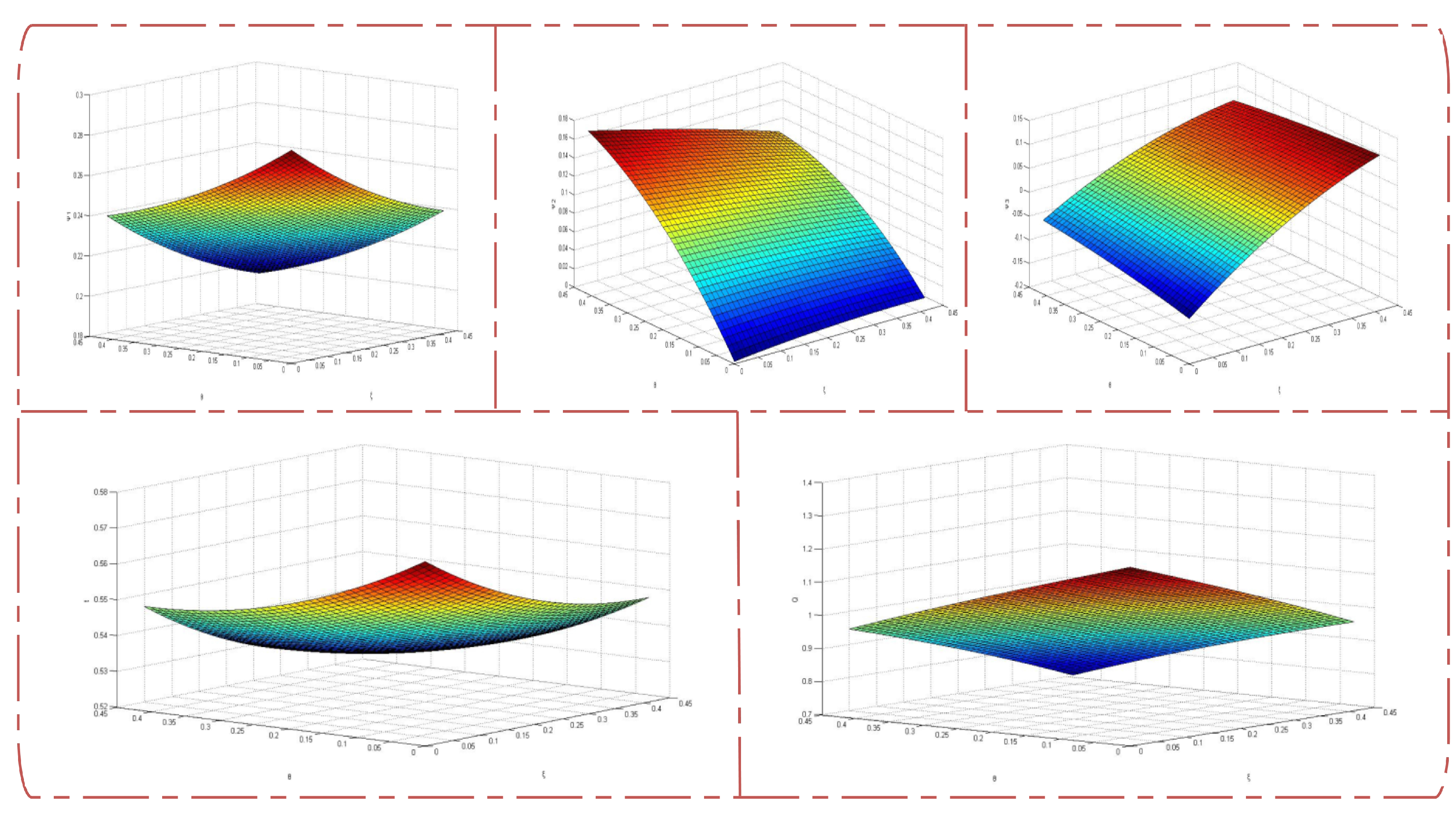
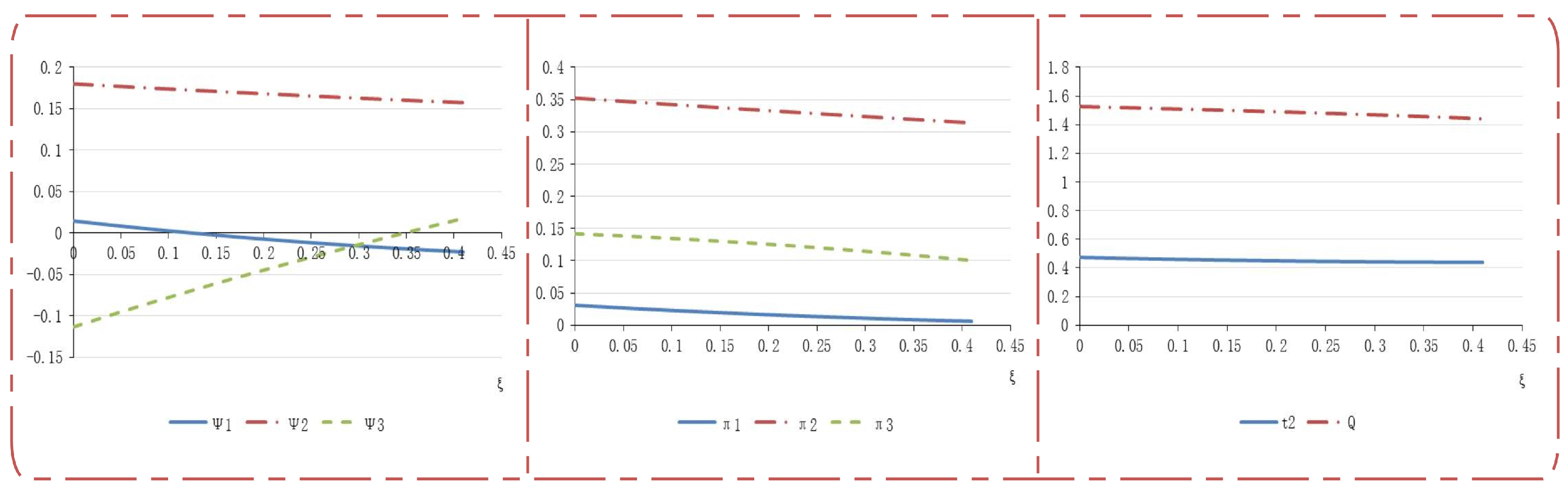
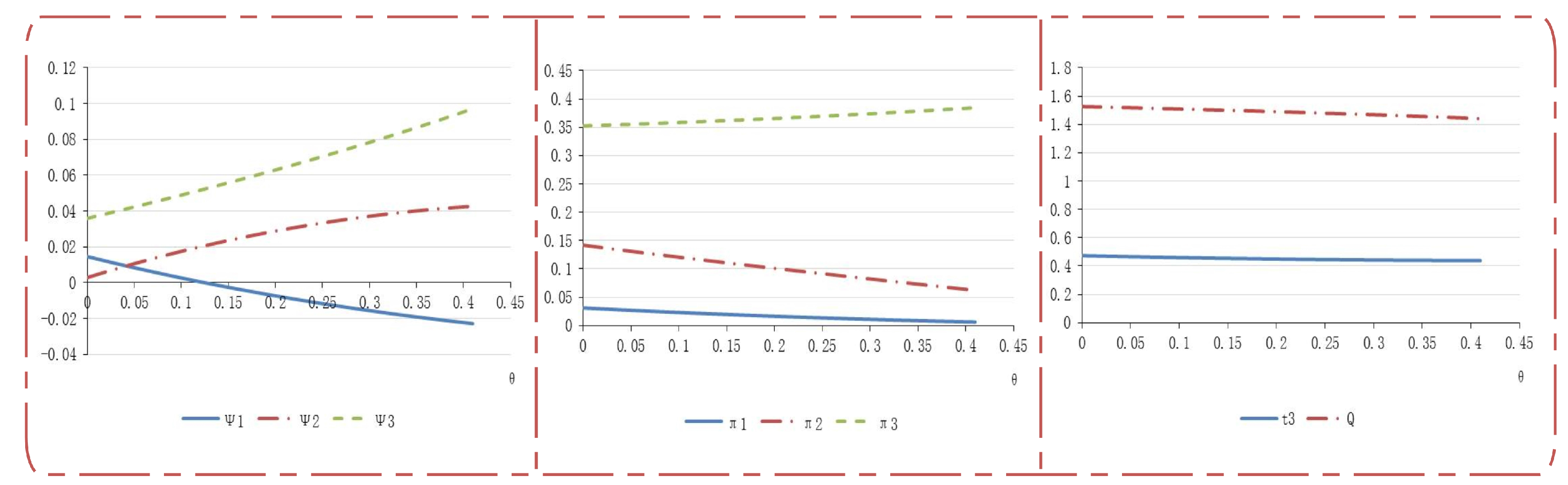
4. Numerical Simulation and Robust Test

4.1. Numerical Simulation

Since the model has a number of parameters, the form of the analytic solution is quite complex, we use numerical simulation to analyze the features of the equilibrium in the form of a numerical solution.

There are eight parameters in the model: a, b, ${\gamma }_1$, ${\gamma }_2$, ${\gamma }_3$, $C_1$, $C_2$, $C_3$, where a and b are parameters of the profit function, $a<0$, $b>0$. Without loss of generality, we standardize parameters and assume $a=-1$, $b=1$. The parameter $C_i$ is assumed to be a minimum with minimal heterogeneity among $C_1$, $C_2$ and $C_3$. Furthermore, the attention to climate change (parameter ${\gamma }_i$) is subject to differences in geographical locations, resource endowment and the level of economic development. We assume that the EU’s attention to climate change is one (${\gamma }_1=1$), which represents the maximum attention to climate with the EU’s status as a forerunner in and staunch advocate for the combat against climate change. Meanwhile, the U.S. and other developed countries, as members of the meddler group, also pay much attention to environmental issues. However, the EU outpaces other developed countries in this aspect. Hence, the attention to climate change of non-EU developed countries (${\gamma }_3$), which is slightly less than that of the EU, is randomly generated and set at 0.90. Since developing countries are still in the period of relatively high-speed economic growth, steps taken for the environment are relatively slower. Thus, ${\gamma }_2$ with a certain gap compared to the developed countries is randomly generated and set at 0.49.

The quantity of carbon dioxide emissions $q_{ij}>0$ and the equilibrium tax rate $t>0$ should be satisfied in each scenario, both of which are merely involved in a, b, ${\gamma }_1$ and have no relevance to ${\gamma }_2$ and ${\gamma }_3$ in the robust test. Therefore, ratios $\theta$ and $\xi$ in retaliatory ACT $\theta t$ and $\xi t$ are given by Equation (52):

$$\begin{array}{c}0<\theta <\frac{2\sqrt{54}-14}{3},0<\xi <\frac{\sqrt{79}-7}{3}\hfill \end{array}$$

(52)

Hence, the ranges of $\theta$ and $\xi$ are: $0<\theta <0.41$, $0<\xi <0.63$. In the reality of international taxation, the tax rate should be set within an appropriate range, as an unreasonably high rate is more likely to enrage airline unions. Thus, both ratio ranges are set from 0–0.41. According to the database of Civil Aviation Administration of China and based on the plan of the EU ETS, the tax rate of the EU ACT is estimated to be 15% at the beginning and then gradually grows to 18%, which proves that the ranges are reasonable. Results are shown in the figures as follows.

Figure 2 shows the impact of $\xi$ ($0<\xi <0.41$), which is the ratio of retaliatory ACT imposed by Meddler 3, on the revenues of countries and airlines, the optimal tax rate of Challenger 1 and the quantity of total carbon dioxide emissions in Model 2 (R, A).

Figure 2 illustrates that the national revenues of Challenger 1 and Defender 2, the revenues of airlines, the optimal tax rate of Challenger 1 and the quantity of total carbon dioxide emissions decrease as $\xi$ increases. The national revenue of Meddler 3 increases as Meddler 3 imposes retaliatory ACT.

Similarly, Figure 3 shows the impact of $\theta$ ($0<\theta <0.41$), which is the ratio of retaliatory ACT imposed by Defender 2, on the revenues of countries and airlines, the optimal tax rate of Challenger 1 and the quantity of total carbon dioxide emissions in Model 3 (A, R).

Figure 3 illustrates that the national revenues of Challenger 1, the revenues of Airlines 1 and 2, the optimal tax rate of Challenger 1 and the quantity of total carbon dioxide emissions decrease as $\theta$ increases. However, the revenues of Defender 2, Meddler 3 and Airline 3 increase. Most notably, the revenues of Meddler 3 and its Airline 3 also increase with the increase of $\theta$.

Figure 4 shows the impact of both $\xi$ and $\theta$ on the revenues of three countries, the optimal tax rate of Challenger 1 and the quantity of total carbon dioxide emissions in Model 4 (A, A) including scenarios (N, A), (A, N) and (A, A).

It can be concluded that the revenues of Challenger 1, Airlines 1 2 and 3, the optimal tax rate of Challenger 1 and the quantity of total carbon dioxide emissions decrease with the increase of $\xi$ and $\theta$, reaching the maximum when $\theta =0.41$, $\xi =0.41$ and falling to the bottom when $\theta =0$ and $\xi =0$.

However, Defender 2 reaches the maximum revenue when $\theta =0.41$, $\xi =0$, because Defender 2 imposes the maximum of ACT in this situation with the lowest tax rate of zero of Meddler 3. Similarly, the maximum revenue of Meddler 3 happens when $\theta =0$, $\xi =0.41$.

Furthermore, since the tax rate of Challenger 1 reaches the top when $\theta =0$, $\xi =0$, the revenues of Defender 2 and Meddler 3 are the minimum. Moreover, the line of the graph with the situation ($\theta =0$, $\xi$ from 0–0.41,) illustrates the trend of the revenue of Defender 2 in scenario (N, A). Similarly, the line with the situation ($\xi =0$, $\theta$ from 0–0.41) illustrates the trend of the revenue of Defender 2 in scenario (A, N). The situations for the revenue of Meddler 3 are the same, for (N, A) and (A, N) are special circumstances of scenario (A, A).

There are only four scenarios (R, R), (R, A), (A, R), (A, A) left and all composed of strategy R and strategy A because the scenarios involved in strategy N are special circumstances of scenarios with strategy A. In this way, further analysis can be conducted in three steps.

To start with, we analyze the revenues of Defender 2 in (R, A) and (A, A) when the strategy of Meddler 3 is fixed as ACT retaliation (A). The revenue of Defender 2 reaches the maximum when $\theta$ is 0.41 regardless of how much tax Meddler 3 imposes. Consequently, the revenue range in (R, A) needs to be compared with the maximum range of revenue in (A, A) ($\theta =0.41$, $\xi$ from 0–0.41). Apparently, the revenue range in (R, A) (0.1801,0.1574) is greater than the maximum revenue range in (A, A) (0.1761,0.1177). Therefore, the best choice for Defender 2 is strategy R.

Additionally, when Meddler 3 chooses strategy R, the revenue range of Defender 2 in (A, R), from 0.0028–0.0427, is permanently less than 0.0740 in (R, R). Therefore, strategy R becomes the optimal strategy for Defender 2 in any cases.

Finally, under the condition that Defender 2 prefers strategy R, we only analyze the revenues of Meddler 3 in Model 1 and Model 2. A majority of the revenue of Meddler 3, who has the power to decide when choosing strategy A, in (A, R) is greater than the revenue in (R, R). Hence, Meddler 3 will give preference to strategy A for Meddler 3 when comparing (R, R) and (R, A).

Figure 5 shows the comparison of the revenue range of Defender 2 in scenarios (R, A) and (A, A) ($\theta$ = 0.41) and the comparison of the revenue range of Defender 2 in scenarios (R, R) and (R, A).

To accurately compare revenues and choose strategies, we use the payoff matrix of Defender 2 (D2 in the table) and Meddler 3 (M3 in the table) to analyze the Nash equilibrium (Challenger 1 will not be discussed here because Challenger 1 goes first and loses the power of decision making).

Table 1. Choices of strategies depending on the range of ${\gamma }_i$. D2, Defender 2; M3, Meddler 3. (The optimal strategies of each scenario comparison are underlined in the payoff matrix following the above analysis)

		M3
		R	A
D2	R	0.0740, $-0.0909$	(0.1574,0.1801), ($-0.1052$,0.0177)
	A	(0.0028,0.0427), (0.0359,0.0972)	(0.1177,0.1761), ($-0.1052,0.1257$)

lists the revenues in the payoff matrix following the above three-step analysis.

From the payoff matrix, the Nash equilibrium is scenario (R, A).

In summary, under the circumstance ${\gamma }_2$ = 0.90, ${\gamma }_3$ = 0.49, Defender 2 (developing countries) prefers refusal of payment, while Meddler 3 (non-EU developed countries) prefers ACT retaliation.

4.2. Robust Test

Since the revenue function of Challenger 1 and airlines does not contain ${\gamma }_2$ and ${\gamma }_3$, the revenues of Challenger 1 and airlines will remain unchanged throughout the robust test.

Choices of strategies depending on the range of ${\gamma }_i$ are discussed by the thresholds of revenues in different scenarios for Defender 2 and Meddler 3.

$$Meddler 3\left\{\begin{array}{c}refusal of payment:{\psi }_{2(R,R)}>{\psi }_{2(A,R)max},{\gamma }_2\in \left(0,0.6759\right)\hfill \\ retaliatory ACT\xi :{\psi }_{2(R,A)min}>{\psi }_{2(A,A)max},{\gamma }_2\in \left(0,0.3947\right)\hfill \end{array}\right.$$

(53)

$$Defender 2\left\{\begin{array}{c}refusal of payment:{\psi }_{3(R,R)}>{\psi }_{3(R,A)max},{\gamma }_3\in \left(0,0.2565\right)\hfill \\ retaliatory ACT\theta :{\psi }_{3(A,R)min}>{\psi }_{3(A,A)max},{\gamma }_3\in \left(0,0.5077\right)\hfill \end{array}\right.$$

(54)

Based on the comparison of revenues and the range of ${\gamma }_i$ above, it is easier to come to a certain conclusion when the minimum revenue of one scenario is greater than the maximum revenue of the other. After that, the remaining choices will be inferred in several steps and be determined when conclusions from two perspectives (row and column in the table) are the same. Results are concluded in

Table 2. Choices of strategies depending on the range of ${\gamma }_i$.

	${\mathit{\gamma }}_1$	(0, 0.2565)	[0.2565, 0.5077]	(0.5077, 1)
${\mathit{\gamma }}_2$
(0, 0.3947)		(R, R)	$(\mathrm{R},\mathrm{A})$	$(\mathrm{R},\mathrm{A})$
[0.3947, 0.6759]		(R, R)	$(\mathrm{R},\mathrm{A})$	$(\mathrm{R},\mathrm{A})$
(0.6759, 1)		$(\mathrm{A},\mathrm{R})$	$(\mathrm{A},\mathrm{R})$	$(\mathrm{A},\mathrm{A})$

Note: The first several steps are given as examples and underlined.

.

Take the first several steps (underlined in Table 2) for example. First of all, when ${\gamma }_2<0.3947$, in the case of Meddler 3 imposing retaliatory ACT $\xi$, the minimum revenue with scenario (R, A) is greater than the maximum revenue with scenario (A, A) for Defender 2 with reference to Equation (53). As 0.3947 is less than 0.6759, according to Equation (53), the revenue with scenario (R, R) is greater than the maximum revenue with scenario (A, R) for Defender 2 under the condition that Meddler 3 chooses refusal of payment and does not impose ACT retaliation $\xi$. Consequently, strategy R is the optimal choice of Defender 2 when ${\gamma }_2<0.3947$, regardless of what strategy Meddler 3 chooses. Second, in the case of Defender 2 choosing strategy R (refusal of payment and no ACT retaliation $\theta$), according to Equation (54), the revenue with scenario (R, R) is greater than the maximum revenue with scenario (R, A) for Meddler 3 when threshold ${\gamma }_3<0.2565$. Thus, the result is scenario (R, R) (Row 2 Column 2 in Table 2).

Similarly, in the case of ${\gamma }_3<0.2565$, with reference to Equation (54), the best choices for Meddler 3 are (R, R) and (A, R) respectively when Defender 2 does not impose ACT retaliation $\theta$ and chooses to impose retaliatory ACT $\theta$ respectively, which means Meddler 3 chooses refusal of payment and does not impose ACT retaliation $\xi$ when threshold ${\gamma }_3$ is less than 0.2565. In the event of Meddler 3 choosing strategy R, according to Equation (53), the revenue with scenario (R, R) (Row 2 and 3 Column 2 in Table 2) is greater than the maximum revenue with scenario (A, R) when ${\gamma }_2<0.6759$.

Table 2 shows that the range of the attention to climate change ${\gamma }_i$ largely influences the choices of strategies. Therefore, Defender 2 and Meddler 3 need to weight ${\gamma }_i$ and estimate the range when making decisions. As meddlers represented by the U.S. and its followers pay at present much attention to climate change, ${\gamma }_3$ falls with high probability within the range (0.5077,1), in which Meddler 3 will choose ACT retaliation. Given that developing countries or emerging economies are mostly in a transitional phase, with the range of [0.3947,0.6759], Defender 2 prefers refusal of payment, which has been discussed by means of numerical simulation.

5. Discussion and Policy Implications

This paper conducts a systematic study of the ACT in a structural framework from a new perspective considering players as belonging to three groups (the EU, developing countries and non-EU developed countries), which distinguishes itself from past research and studies on the ACT from a dual perspective (EU and non-EU countries).

To begin with, this paper analyzes nine scenarios by two-stage game models with three possible strategies (non-resistance, refusal of payment and ACT retaliation). Based on Nash equilibriums in four models, an analysis is made about the revenues of countries and airlines, the optimal tax rate and the quantity of emissions.

After analyzing nine scenarios and modeling two-stage games, results are visualized by means of the numerical simulation with tables and figures, which clearly illustrate the relationship among variables. We also apply the robust test for an examination of the robustness.

As a result, this paper theoretically verifies that refusal of payment of the aviation carbon tax is an appropriate strategy for emerging economies. Since developing countries, as major defenders, are experiencing relatively rapid economic growth at present and still have gaps compared to developed countries on the attention paid to climate change, refusal of payment is the strategy that benefits both the nations and their domestic airlines.

As for meddlers represented by the U.S. and other non-EU developed countries, imposing the ACT at an appropriate level is an ideal choice. On the one hand, developed countries pay more attention to environmental problems. On the other hand, the unilateral ACT of the EU will damage the national revenues of other countries including non-EU developed countries. If non-EU developed countries impose ACT retaliation, it will benefit all groups to a certain extent. However, the tax rate should be carefully determined, in light of the rights and power of aviation unions in safeguarding profits for airlines.

More precisely, developing countries are mostly in a transitional phase. Since the attention paid to climate change has not yet approached thresholds, they prefer refusal of payment. According to robust analysis, emerging economies will tend to impose ACT retaliation like developed countries after reaching the critical value.

The results above have practical implications for policy. After developing countries start imposing ACT retaliation, it will become similar to the MBM scheme. In the MBM framework, members will sign with each other bilateral or multilateral agreements, which, coupled with appropriate strategies, will lead to mutual benefits within the MBM framework.

In fact, MBM is taken as a relatively preferable choice at present for two reasons. Firstly, there is no possibility for unilateral imposition because non-resistance is eliminated as a strictly dominated strategy, and it is therefore better for nations and economies to participate in a multilateral scheme. Secondly, ICAO, as an international organization, guarantees that countries sign agreements by weighing their own statuses and national conditions and those of other contracting states within a global unified strategic framework, which is less likely to be accused of injustice.

It is worth stressing that it may be possible for the MBM scheme to consider following the example of the WTO and to provide a transitional period lasting several years for developing countries and emerging economies. Although developing countries are generally willing to shoulder their responsibility to curb emissions to meet global goals, they will need time to reach thresholds of the attention to climate change ${\gamma }_i$. Therefore, a period of transition is necessary for emerging economies. For example, China has gained a fifteen-year transition from the WTO to improve domestic market and legislation, which has not only contributed to the reform in China, but also positively influenced the world economy. The ACT faces similar circumstances. Developing countries will continuously adjust domestic environmental policies during the transitional period until reaching the thresholds, upon which they may start imposing the ACT. Thus, the development of the ACT will essentially enter into a new and sustainable stage with MBM bilateral or multilateral agreements.

This paper has developed a new structural framework with three groups to analyze carbon taxation of the global emission issue, which can be widely applied to situations where a player adopts the same policies for other players while facing distinct treatments from them. Hence, nations or economies are generalized into three groups rather than only two groups, i.e., the EU and non-EU countries.

First of all, a tripartite perspective is closer to reality. The framework of three groups loosens assumptions, which is more appropriate for a complex international situation with the presence of mutual restraints and interactivity. To be exact, any nations or economies can be involved in the three groups in the framework of this paper, where countries take all related parties into consideration when making decisions.

Most importantly, the taxation framework for solving global emission problems is different from other taxation schemes. The global climate change issue is regarded as a distinct responsibility or duty for all countries instead of a generator of revenues or benefits. Therefore, the carbon taxation policy of one state should treat other groups equally without discrimination to avoid objections and conflicts, which is different from the circumstances with the international taxation or the tariff. The following example with a random set of three countries (A, B and C) illustrates this point. In international taxation, Country C can use different strategies of tax credits or provide extra preferential reductions on the tax rate to Country A and Country B due to economic, geographic and other factors. Thus, Country A and Country B will adopt different policies for Country C based on their bilateral agreements. Besides, the cases are similar in the customs tariff, where alliances are formed as regional organizations to achieve mutual benefits within the alliances by policies such as the national treatment. However, in the field of carbon emissions, Country C should treat A and B equally even if C observes A and B taking different ACT policies. Since the ACT is a global climate duty for all countries, only one country imposing ACT will not spark conflicts. In general, the “three groups” situation can be simplified into three “two sides” situations, which can be studied by the framework of games with two players; in the case of global unified strategies, it involves a complete tripartite perspective and framework.

Through the explicit modeling of two-stage games of nine scenarios on the ACT issue, the structural framework with three groups here can be applied to analyze other similar situations where a player adopts the same actions or policies for other players while facing distinct treatments from them; it also can be used as a basis for even more sophisticated models with complex relationships among the players, which may provide a general perspective to analyze other empirical applications from a tripartite framework. To achieve sustainability, it will be of more practical value to include all nations and economies based on a complete tripartite perspective.

6. Conclusions

In conclusion, this paper analyzes nine scenarios by two-stage game models with three possible strategies for nations and economies generalized into three groups. It is “mutual benefits” rather than “zero sum” for the EU, developing countries and non-EU developed countries on the ACT. Based on the Nash equilibrium, the numerical simulation and the robust test, the ACT can be imposed effectively and efficiently through multilateral agreements of the MBM scheme proposed by ICAO. More specifically, the EU will most probably continue to impose the ACT, and non-EU developed countries, such as the U.S., will impose ACT retaliation at an appropriate tax rate. At present, refusal of payment of ACT is a practical strategy for developing countries. However, they will tend to impose the ACT like developed countries after reaching thresholds of the attention to climate change. Hence, we suggest a period of transition for emerging economies included in the MBM scheme.

By generalizing players into three groups, this paper develops a systematic study of carbon taxation on the global emission issue in a structural framework. In addition to the tripartite perspective loosening assumptions and approaching reality, the game framework can be extended to other situations, as well. Finally, this paper underlines the importance of multilateral corporation for nations and economies in a bid for global sustainability.

References

1. Babiker, M.H.; Rutherford, T.F. The economic effects of border measures in subglobal climate agreements. Energy J. 2005, 26, 99–126. [Google Scholar] [CrossRef]
2. Asselt, H.V.; Brewer, T. Addressing competitiveness and leakage concerns in climate policy: An analysis of border adjustment measures in the US and the EU. Energy Policy 2010, 38, 42–51. [Google Scholar] [CrossRef]
3. Dissou, Y.; Eyland, T. Carbon control policies, competitiveness, and border tax adjustments. Energy Econ. 2011, 33, 556–564. [Google Scholar] [CrossRef]
4. Eyland, T.; Zaccour, G. Strategic effects of a border tax adjustment. Int. Game Theory Rev. 2012, 14, 1–22. [Google Scholar] [CrossRef]
5. Sakai, M.; Barrett, J. Border carbon adjustments: Addressing emissions embodied in trade. Energy Policy 2016, 92, 102–110. [Google Scholar] [CrossRef]
6. Ibitz, A. Towards a global scheme for carbon emissions reduction in aviation: China’s role in blocking the extension of the European Union’s Emissions Trading Scheme. Asia Eur. J. 2015, 13, 113–130. [Google Scholar] [CrossRef]
7. Anger, A. Including aviation in the EU ETS: Impacts on the industry, CO2 emissions and macroeconomic activity in the EU. J. Air Transp. Manag. 2010, 16, 100–105. [Google Scholar] [CrossRef]
8. Anger, A.; Köhler, J. Including aviation emissions in the EU ETS: Much ado about nothing? A review. Transp. Policy 2010, 17, 38–46. [Google Scholar] [CrossRef]
9. Yoon, S.; Jeong, S. Carbon Emission Mitigation Potentials of Different Policy Scenarios and Their Effects on International Aviation in the Korean Context. Sustainability 2016, 8, 1179. [Google Scholar] [CrossRef]
10. Scheelhaase, J.D.; Grimme, W.G. Emissions trading for international aviation—An estimation of the economic impact on selected European airlines. J. Air Transp. Manag. 2007, 13, 253–263. [Google Scholar] [CrossRef]
11. Scheelhaase, J.; Grimme, W.; Schaefer, M. The inclusion of aviation into the EU emission trading scheme—Impacts on competition between European and non-European network airlines. Transp. Res. Part D Transp. Environ. 2010, 15, 14–25. [Google Scholar] [CrossRef]
12. Vorster, S.; Ungerer, M.; Volschenk, J. 2050 Scenarios for long-haul tourism in the evolving global climate change regime. Sustainability 2012, 5, 1–51. [Google Scholar] [CrossRef]
13. Sharp, H.; Grundius, J.; Heinonen, J. Carbon Footprint of Inbound Tourism to Iceland: A Consumption-Based Life-Cycle Assessment including Direct and Indirect Emissions. Sustainability 2016, 8, 1147. [Google Scholar] [CrossRef]
14. Higham, J.; Cohen, S.A.; Cavaliere, C.T.; Reis, A.; Finkler, W. Climate change, tourist air travel and radical emissions reduction. J. Clean Prod. 2016, 111, 336–347. [Google Scholar] [CrossRef]
15. Mayor, K.; Tol, R.S.J. The impact of the UK aviation tax on carbon dioxide emissions and visitor numbers. Transp. Policy 2007, 14, 507–513. [Google Scholar] [CrossRef]
16. Tol, R.S.J. The impact of a carbon tax on international tourism. Transp. Res. Part D Transp. Environ. 2007, 12, 129–142. [Google Scholar] [CrossRef]
17. Shi, Y.B. Reducing greenhouse gas emissions from international shipping: Is it time to consider market-based measures? Mar. Policy 2016, 64, 123–134. [Google Scholar] [CrossRef]
18. Psaraftis, H.N. Green Maritime Transportation: Market Based Measures; Chapter Green Transportation Logistics; Springer International Publishing: Cham, Switzerland, 2016; pp. 267–297. [Google Scholar]
19. Liang, S.; Zhu, L.; Ming, X.; Zhang, T.Z. Waste oil derived biofuels in China bring brightness for global GHG mitigation. Bioresour. Technol. 2013, 131, 139–145. [Google Scholar] [CrossRef] [PubMed]
20. Moghaddam, R.F.; Moghaddam, F.F.; Cheriet, M. A modified GHG intensity indicator: Toward a sustainable global economy based on a carbon border tax and emissions trading. Energy Policy 2013, 57, 363–380. [Google Scholar] [CrossRef]
21. Arjomandi, A.; Seufert, J.H. An evaluation of the world’s major airlines’ technical and environmental performance. Econ. Model. 2014, 41, 133–144. [Google Scholar] [CrossRef]
22. Meunier, G.; Ponssard, J.P.; Quirion, P. Carbon leakage and capacity-based allocations: Is the EU right? J. Environ. Econ. Manag. 2014, 68, 262–279. [Google Scholar] [CrossRef]
23. Hering, L.; Poncet, S. Environmental policy and exports: Evidence from Chinese cities. J. Environ. Econ. Manag. 2014, 68, 296–318. [Google Scholar] [CrossRef]
24. Trotter, I.M.; Cunha, D.A.D.; Féres, J.G. The relationships between CDM project characteristics and CER market prices. Ecol. Econ. 2015, 119, 158–167. [Google Scholar] [CrossRef]
25. Sun, C.W.; Yuan, X.; Yao, X. Social acceptance towards the air pollution in China: Evidence from public’s willingness to pay for smog mitigation. Energy Policy 2016, 92, 313–324. [Google Scholar] [CrossRef]
26. Markandya, A.; Ricci, E.C. Green Taxes on Aviation: The Case of Italy. The Proposal of the Green Taxation Matrix; Chapter Environmental Taxes and Fiscal Reform; Palgrave Macmillan: London, UK, 2012; pp. 168–206. [Google Scholar]
27. Peterson, E.B.; Lee, H.L. Implications of incorporating domestic margins into analyses of energy taxation and climate change policies. Econ. Model. 2009, 26, 370–378. [Google Scholar] [CrossRef]
28. Bassi, A.M.; Yudken, J.S. Climate policy and energy-intensive manufacturing: A comprehensive analysis of the effectiveness of cost mitigation provisions in the American Energy and Security Act of 2009. Energy Policy 2011, 39, 4920–4931. [Google Scholar] [CrossRef]
29. Carfì, D.; Schilirò, D. A coopetitive model for the green economy. Econ. Model. 2012, 29, 1215–1219. [Google Scholar] [CrossRef]
30. Jayanthakumaran, K.; Liu, Y. Bi-lateral CO2 emissions embodied in Australia-China trade. Energy Policy 2016, 92, 205–213. [Google Scholar] [CrossRef]
31. Wang, Q.W.; Su, B.; Zhou, P.; Chiu, C.R. Measuring total-factor CO2 emission performance and technology gaps using a non-radial directional distance function: A modified approach. Energy Econ. 2016, 56, 475–482. [Google Scholar] [CrossRef]
32. Gong, C.Z.; Yu, S.W.; Zhu, K.J.; Hailu, A. Evaluating the influence of increasing block tariffs in residential gas sector using agent-based computational economics. Energy Policy 2016, 92, 334–347. [Google Scholar] [CrossRef]
33. Fitzgerald, J.; Tol, R.S.J. Airline emissions of carbon dioxide in the European Trading System. CESifo Forum 2007, 1, 51–54. [Google Scholar]
34. Mayor, K.; Tol, R.S.J. European Climate Policy and Aviation Emissions; ESRI Working Paper No. 241; ESRI Publishing: Dublin, Ireland, 2008. [Google Scholar]
35. Mayor, K.; Tol, R.S.J. Scenarios of carbon dioxide emissions from aviation. Glob. Environ. Chang. 2010, 20, 65–73. [Google Scholar] [CrossRef]
36. Elliott, J.; Weisbach, D. Trade and carbon taxes. Am. Econ. Rev. 2010, 100, 465–469. [Google Scholar] [CrossRef]
37. Mcmanners, P.J. Developing policy integrating sustainability: A case study into aviation. Environ. Sci. Policy 2016, 57, 86–92. [Google Scholar] [CrossRef]
38. Gunasekara, S.G. Environmental overreach: The EU’s carbon tax on international aviation. Wash. Lee J. Energy Clim. Environ. 2013, 5, 1. [Google Scholar]
39. Horn, H.; Sapir, A. Can Border Carbon Taxes Fit into the Global Trade Regime? Policy Briefs 805; Bruegel Publishing: Brussels, Belgium, 2013. [Google Scholar]
40. Keen, M.; Strand, J. Indirect taxes on international aviation. Fisc. Stud. 2007, 28, 1–41. [Google Scholar] [CrossRef]
41. Karp, L.; Zhang, J.F. Taxes versus quantities for a stock pollutant with endogenous abatement costs and asymmetric information. Econ. Theory 2012, 49, 371–409. [Google Scholar] [CrossRef]
42. Zhang, X.B.; Zhu, L. Strategic carbon taxation and energy pricing under the threat of climate tipping events. Econ. Model. 2017, 60, 352–363. [Google Scholar] [CrossRef]
43. Wu, P.I.; Chen, C.T.; Cheng, P.C.; Liou, J.L. Climate game analyses for CO2 emission trading among various world organizations. Econ. Model. 2014, 36, 441–446. [Google Scholar] [CrossRef]
44. Qiao, H.; Song, N.; Lu, B.; Hua, G.W.; Du, H.S. China’s optimal strategy against the European Union aviation carbon tax scheme: A two-stage game model analysis. Environ. Eng. Manag. J. 2015, 14, 1803–1811. [Google Scholar]
45. Li, M.; Gao, G.K.; Wang, Y.C. International aviation carbon taxation: Game between EU and Non-EU countries. Adv. Appl. Econ. Financ. 2012, 3, 546–551. [Google Scholar]
46. Dong, J.; Ma, Y.; Sun, H. From Pilot to the National Emissions Trading Scheme in China: International Practice and Domestic Experiences. Sustainability 2016, 8, 522. [Google Scholar] [CrossRef]
47. Choi, Y.; Lee, H.S. Are Emissions Trading Policies Sustainable? A Study of the Petrochemical Industry in Korea. Sustainability 2016, 8, 1110. [Google Scholar] [CrossRef]
48. Barrett, S. Self-enforcing international environmental agreements. Oxf. Econ. Pap. 1994, 46, 878–894. [Google Scholar] [CrossRef]
Figure 1. Stage 1 of the game in extended expression. N, non-resistance; R, refusal of payment; A, aviation carbon tax (ACT) retaliation.
Sustainability 09 01247 g001
Figure 2. Revenues of countries, revenues of airlines, optimal tax rate of Challenger 1 and quantity of total carbon dioxide emissions in Model 2.
Sustainability 09 01247 g002
Figure 3. Revenues of countries, revenues of airlines, optimal tax rate of Challenger 1 and quantity of total carbon dioxide emissions in Model 3.
Sustainability 09 01247 g003
Figure 4. Revenue of Challenger 1, revenue of Defender 2, revenue of Meddler 3, optimal tax rate of Challenger 1 and the quantity of total carbon dioxide emissions in Model 4.
Sustainability 09 01247 g004
Figure 5. Comparison of the revenue range of Defender 2 in (R, A) and (A, A) ( θ = 0.41) and the comparison of the revenue range of Meddler 3 in (R, A) and (A, A) ( θ = 0.41).
Sustainability 09 01247 g005