Economic and Environmental Performance of Fashion Supply Chain: The Joint Effect of Power Structure and Sustainable Investment

Abstract

Fashion supply chain members now search for trade-offs between sustainable investment and the related incentives, such as savings on environmental taxes and gains in incremental demands. To evaluate the economic and environmental performance of sustainable investment from a power perspective, we develop an analytical model to study a two-echelon sustainable supply chain consisting of one retailer and one manufacturer with three different power structures. We derive the optimal solutions for various cases associated with different supply chain power structures and sustainable investors. Though it is beneficial for both the manufacturer and retailer to make sustainable investment, they often utilize high power to gain economic benefit with less sustainable investment. Interestingly, the follower with less supply chain power has more incentive to make a sustainable effort to achieve a higher profit. The optimal amount of sustainable investment in the apparel manufacturer investment case is greater than that in the retailer investment case in most scenarios.

1. Introduction

Global textile consumption is estimated at more than 30 million tons per year, which causes serious environmental impact within the fashion supply chain [1]. Facing increasingly crucial environmental issues in fashion industries, many fashion brands have developed pollution-abatement technologies and sustainable designs, which require substantial investments [2]. The costly investments usually cannot be justified by purely economic indicators, and some incentives are provided by environmental policy and market response (Krass et al. [3]). Regarding the policy, environmental tax is often used as an efficient tool to promote firms to invest in sustainable effort to control the pollution (Atasu et al. [4], Drake et al. [5], Krass et al. [3]). For instance, the solar Investment Tax Credit (ITC) is used to support the deployment of solar energy in the United States. It is currently a 30% federal tax credit claimed against the tax liability of residences and allows the homeowner to apply the credit to his/her personal income taxes. Regarding the market response, a number of studies have shown that the sustainable practices have positive effect on the market demand (see, e.g., Swami and Shah [6], Shen [7], Tang et al. [8], Dong et al. [9], and Li and Shen [10]). This phenomenon is also widely observed in real practice, especially in fashion industry. For example, consumers are willing to purchase the H&M’s organic cotton t-shirts, even if these sustainable products are relatively more expensive than the regular ones [7].

Based on these facts, on the one hand, fashion companies have more incentive to invest in sustainable design [7,10]. Well-known examples include the sustainability practices in H&M, which is the second largest user of recycled polyester in the world and used recycled polyester equivalent to more than 180 million Polyethylene terephthalate (PET) bottles in 2016 [11]. On the other hand, it is also significant for companies to look beyond their organizational boundaries and develop a more efficient solution for a sustainable supply chain. Accordingly, sustainable supply chain practices are also observed in retail industry. For example, Marks & Spencer, the largest retail group in UK, invested 200 million pounds on a sustainable project called “Plan A” in 2007. This sustainable project, which consists of 100 commitments to achieve environmental goals, covers Marks & Spencer and its suppliers. According to the annual report of Plan A in 2016, 42% of the cotton sourced by suppliers for Marks & Spencer products came from sustainable sources (32% in the previous year), and their aim is to improve it to 70% before 2020 [12].

From the above observations, both apparel manufacturers and retailers search for trade-offs between sustainable investment and the related incentives, such as savings on environmental taxes and gains in incremental demands. Sometimes, core enterprises, such as H&M and Marks & Spencer, involve their supply chain partners in their sustainable projects. It is important to investigate the economic and environmental performance of sustainable investment by manufacturers and retailers. In addition, it is interesting to investigate whether the fashion supply chain partners with less power are hurt or benefit when they participate in supply chain leaders’ sustainable projects.

Very little effort has been made in the existing literature to explore the issue of sustainable investment in a supply chain with the consideration of power structure, except Chen et al. [13], who however did not consider that the retailer may invest the sustainable effort. In this paper, we aim to investigate the joint effort of power structure and sustainable investment on the economic and environmental performance of supply chains. We consider a fashion supply chain consisting of one retailer and one manufacturer, and both of them have options to invest in sustainable effort. Following the industrial practices, we consider that the sustainable investment will bring a decrease of tax and an increase of demand. We analyze the retailer’s and manufacturer’s sustainable investment and pricing decisions in manufacturer Stackelberg (MS) model, the vertical Nash (VN) model, and the retailer Stackelberg (RS) model, respectively. We derive the optimal solutions for various cases associated with these three supply chain power structures and two different sustainable investors. Besides, by conducting some comparisons, we obtain some important managerial insights. To the best of our knowledge, this paper is the first to study the effects of sustainable investment by different investors in supply chains with different power structures. We show that it can be beneficial for both the manufacturer and retailer to make sustainable investment, especially for the follower with less supply chain power. The optimal amount of sustainable investment in the manufacturer investment case is greater than that in retailer investment case in either VN or RS supply chain structure. In a MS structure, the retailer is willing to make more investment than the manufacturer does, if the sustainable sensitivity of demand is relatively high.

The rest of the paper is organized as follows. In Section 2, we conduct a literature review. In Section 3, we introduce the three models of different sustainable investors. In Section 4 and Section 5, we analyze the optimal solutions with the manufacturer’s sustainable investment and the retailer’s sustainable investment settings, respectively. All of the optimal solutions in different structures are compared and managerial insights are derived in these two sections. In Section 6, we compare the different investors’ sustainable investment decisions and related performance. Section 7 concludes the paper. All proofs are relegated to the Appendix A.

2. Literature Review

Our work is related to two streams of the research in the operations management/operations research literature. The first stream is the literature taking the sustainability issue into consideration. The second stream is the literature considering the impact of the power structure.

Sustainability issue has received extensive attention in the operations management and operations research literature, and there is growing consensus that the sustainability issue should be integrated into operational decision (Benjaafar et al. [14], Choi [15], Drake and Spinler [16], Dong et al. [9]). Letmathe and Balakrishnan [17] and Dobos [18] are two early papers that study the production and inventory policies by taking the sustainability issue into consideration. Recently, there are many other papers studying the production and/or inventory management with sustainable effort investment and/or the regulation on the carbon emission consideration (e.g., Bouchery et al. [19], Benjaafar et al. [14], Zhang and Xu [20], Nouira et al. [21], and Toptal et al. [22]). There are also some other papers studying the effects of carbon emission with respect to other issues. For example, Choi [15] addressed how a carbon footprint taxation scheme could be imposed on a fashion quick response system. Rosič and Jammernegg [23] investigated the impact of carbon emission policy on the transportation mode. Yalabik and Fairchild [24], Liu et al. [25], and Chen and Hao [26] studied the effect of carbon emission on operational decisions for firms in a competitive environment. Jaber et al. [27], Zhang et al. [28], Du et al. [29] and Dong et al. [9] considered the supply chain coordination with consumer environmental awareness and/or emissions reduction incentives. Drake et al. [5] analyzed the effects of emission tax and emissions trading regulation on the technology choice and capacity decisions. Li and Shen [10] studied the sustainable design operations by comparing the non-profit manufacturer and for-profit manufacturer business modes in fashion industry. While also considering consumer environmental awareness and emissions reduction investment, we focus on the joint effects of sustainability issues and power structure in this paper.

In the literature, the supply chain power structure is modeled with respect to the sequence of actions of manufacturer and retailer. The manufacturer Stackelberg game has been widely considered in the literature (Shi et al. [30]). For example, Anupindi and Bassok [31], Lariviere and Porteus [32], Dong and Rudi [33], and Taylor [34] used manufacturer Stackelberg games to study the interaction of supply chain members. The interaction has also been modeled as Vertical Nash game, in which both supply chain members make their decisions simultaneously. Examples can be found in Iyer and Villas-Boas [35], Inderst and Wey [36], etc. To model the situation of a power retailer, there are some papers that consider retailer Stackelberg games, such as Dukes et al. [37], Geylani et al. [38], Raju and Zhang [39], and Wang et al. [40].

Differing from the above literature that mainly focuses on one specific game, there are some papers that study the impacts of the different power structures. Choi [41] analyzed the impact of power structure with the consideration of price competition. Ertek and Griffin [42] explored the impact of power structure in a two-stage supply chain. Majumder and Srinivasan [43] investigated the impact of contract leadership on the performance of supply chain. Nagarajan and Sošić [44] studied the effects of different power structures on dynamic supplier alliances in a decentralized assembly system. Shi et al. [30] analyzed the impacts of power structure on supply chains with uncertain demand. Xue et al. [45] examined how different power structures affect the supply chain performance and consumer surplus. Chen and Wang [46] studied the effects of power structure on the channel selection between a free channel and a bundled channel. Chen et al. [47] investigated the impact of power structure on the retail service in a dual channel supply chain. Chen et al. [48] examined the effects of power structure on the pricing and effort decisions for a supply chain with uncertain information. Zheng et al. [49] studied the impact of the power structure on dual-channel closed-loop supply chain. Chen et al. [13] examined the effect of power structure on the supply chain coordination. In our paper, we study the effect of power structure on the supply chain performance with the consideration of consumer environmental awareness and emissions reduction investment. The majority of above studies did not consider the carbon emission, except Chen et al. [13], who however did not consider that the retailer may invest the sustainable effort, which is different from our study.

Table 1. A summary of closely related literature.

Papers	Sustainability Issues				Power Structure
	Carbon Emission	Sustainable Investment Decision		Consumer Environment Awareness
		Manufacturer Investment Decision	Retailer Investment Decision
Choi [15], Drake and Spinler [16], Dobos [18], Bouchery et al. [19], Rosič and Jammernegg [23], Chen and Hao [26], Jaber et al. [27]	✓
Benjaafar et al. [14], Letmathe and Balakrishnan [17], Zhang and Xu [20]	✓	✓
Toptal et al. [22]	✓		✓
Zhang et al. [28]	✓			✓
Dong et al. [9], Li and Shen [10], Nouira et al. [21], Yalabik and Fairchild [24], Liu et al. [25], Du et al. [29]	✓	✓		✓
Shi et al. [30], Choi [41], Ertek and Griffin [42], Majumder and Srinivasan [43], Nagarajan and Sošić [44], Xue et al. [45], Chen and Wang [46], Chen et al. [47], Chen et al. [48], Zheng et al. [49]					✓
Chen et al. [13]	✓	✓		✓	✓
This paper	✓	✓	✓	✓	✓

summarizes the closely related literature on operations management and operations research with the consideration of sustainability issues and power structure. Regarding the literature on the sustainability issues, it can be found that, even though the existing literature has examined various aspects of sustainability issues, most studies considered that the manufacturer invests the sustainable effort. How retailer’s investment decision affects the economic and environmental performance of the supply chain is not yet fully addressed. Regarding the literature on the power structure, it can be found that the majority of the above literatures did not consider the sustainability issues. However, it is important to investigate the jointly effect of the power structure and sustainability issues on fashion supply chain. Addressing these questions hence outlines the contribution of our study.

3. Modeling Framework

Consider a fashion retailer (she), who purchases single type products from an apparel manufacturer (he) and sells to consumers. The retailer needs to decide the unit selling price $p$. The manufacturer’s unit production cost is $c$, and he decides the unit wholesale price $w$. Clearly, we have $p>w>c$.

In addition, the fashion supply chain members can invest some sustainable effort to improve the functionality of the products. Investing on sustainable effort is costly, but it can make the products be suitable for more needed consumers and reduce pollutant and related environmental taxes. Thus, investment on the sustainable effort has positive effect on the demand (see, e.g., Swami and Shah [6], and Dong et al. [9]). We assume that the market demand is deterministic. Let $D\left(p,e\right)$ be the demand quantity, which equals to the retailer’s ordering quantity.

$$Q=D\left(p,e\right)=\alpha -\beta p+\gamma e.$$

(1)

Notice that the primary effect of the environmental taxation has induced the choice of less environmentally damaging technology alternatives (Dong et al. [9]). Accordingly, we assume that the sustainable effort cuts the apparel manufacturer’s environmental tax, which is denoted as $T\left(e\right)$. For easy exposition of the analysis, we assume that $T\left(e\right)=-te$, where $t$ is determined by tax rate and per unit pollutant emission equivalent. For instance, according to the Chinese Environmental Protection Tax Law, the tax base of atmospheric and water pollutants is determined by the pollution equivalent number, which is converted from the pollutant emission amount and taxable pollutants will be taxed at RMB 1.2 to RMB 12 per pollution equivalent, respectively. Essentially, the sustainable effort reduces environmental tax by controlling per unit pollutant equivalent.

Due to the savings on the environmental tax and the positive effect on the demand, both the retailer and manufacturer have motivation to invest in the sustainable effort. We consider the following investment function:

$$I\left(e\right)=\lambda e^2.$$

(2)

It indicates that the investment is convex, increasing in $e$. This setting is popular in the literature (see, e.g., Savaskan and Van Wassenhove [50], Li et al. [51], and Dong et al. [9]).

To avoid the trivial outcome, we assume that the investment coefficient is high such that $\lambda >{\left(\gamma +\beta t\right)}^2/2\beta$. This is also reasonable because in reality the investment cost for improving the sustainable level is usually high (Dong et al. [9]).

Based on the above settings, we consider two cases: the manufacturer makes sustainable investment, and the retailer makes sustainable investment. Both members’ objectives are to maximize their profits. Let ${\Pi }_r^m$ and ${\Pi }_m^m$ denote the retailer’s and manufacturer’s profits, respectively, when manufacturer makes sustainable investment. Let ${\Pi }_r^r$ and ${\Pi }_m^r$ denote the retailer’s and manufacturer’s profits, respectively, when retailer makes sustainable investment. The profit functions are given as follows:

• The manufacturer makes sustainable investment.

  $${\Pi }_r^m\left(p\right)=\left(p-w\right)Q=\left(p-w\right)\left(\alpha -\beta p+\gamma e\right)$$

  (3)

  $${\Pi }_m^m\left(w,e\right)=\left(w-c-T\left(e\right)\right)Q-I\left(e\right)=\left(w-c+te\right)\left(\alpha -\beta \left(w+m\right)+\gamma e\right)- \lambda e^2$$

  (4)
• The retailer makes sustainable investment.

  $${\Pi }_r^r\left(p,e\right)=\left(p-w\right)Q-I\left(e\right)=\left(p-w\right)\left(\alpha -\beta p+\gamma e\right)- \lambda e^2$$

  (5)

  $${\Pi }_m^r\left(w\right)=\left(w-c-T\left(e\right)\right)Q=\left(w-c+te\right)\left(\alpha -\beta \left(w+m\right)+\gamma e\right)$$

  (6)

Notice that sustainable investment increases market demands, consequently, the retail price and wholesale price have growing trend. Hence, we assume that the sustainable investment is positive related to the retail price and wholesale price. To guarantee this assumption, we assume that $\gamma >\beta t$.

In each investment scenario, we discuss the models with three different fashion supply chain power structures, i.e., the manufacturer Stackelberg (MS) model, the vertical Nash (VN) model, and the retailer Stackelberg (RS) model. These model settings are quite common in fashion industries. For example, H&M usually acts a leader in a supply chain and has dominant position when it deals with retailers. Nike and Adidas have equivalent status with their retailers, such as ASOS and Amazon. These companies announce their sustainable effort on their websites. Their practices well fit the VN model setting. Moreover, the RS model can be observed from Marks & Spencer’s sustainable project called Plan A, in which Marks & Spencer makes sustainable investment and requirement for its supplies [12].

In the case of a MS power structure, the manufacturer and retailer make decisions sequentially. The retailer determines the retailer price and sustainable investment level (if any) in response to a given wholesale price. After observing the retailer’s response, the manufacturer decides the optimal wholesale price and sustainable investment level (if any).

In the case of a VN power structure, the manufacturer and the retailer make decisions simultaneously. The retailer (manufacturer) determines the product price (wholesale price) and sustainable investment level (if any) to maximize profit given a wholesale price (the retail price). Finally, the consumer demand is realized and the supply chain members gain their revenues.

In the case of a RS power structure, the manufacturer and retailer make their decisions in sequence. The manufacturer decides the wholesale price and sustainable investment level (if any) in response to the given a retail price and sustainable investment level (if any). Then, by taking the manufacturer’s response function into account, the retailer determines the optimal retail price and sustainable investment level (if any).

4. The Manufacturer Makes Sustainable Investment

For the manufacturer’s optimal wholesale price (i.e., $w_i^m$) and sustainable effort (i.e., $e_i^m$), and the retailer’s optimal retail price (i.e., $p_i^m$) in different power structures ($i=m,n,r$ standing for MS, VN and RS models, respectively), we obtain the following lemma:

Lemma 1.

The manufacturer’s optimal wholesale price and sustainable effort, and retailer’s optimal price in three different power structures are summarized in

Table 2. Optimal decision when the manufacturer makes sustainable investment.

Model	${\mathit{p}}_{\mathit{i}}^{\mathit{m}}$	${\mathit{e}}_{\mathit{i}}^{\mathit{m}}$	${\mathit{w}}_{\mathit{i}}^{\mathit{m}}$
MS Model ($i=m$)	$c+\frac{\left(6\lambda -\beta t^2-t\gamma \right)\left(\alpha -\beta c\right)}{8\lambda \beta -{\left(\gamma +t\beta \right)}^2}$	$\frac{\left(\gamma +t\beta \right)\left(\alpha -\beta c\right)}{8\lambda \beta -{\left(\gamma +t\beta \right)}^2}$	$c+\frac{\left(4\lambda -\beta t^2-t\gamma \right)\left(\alpha -\beta c\right)}{8\lambda \beta -{\left(\gamma +t\beta \right)}^2}$
VN Model ($i=n$)	$c+\frac{\left(4\lambda -\beta t^2-t\gamma \right)\left(\alpha -\beta c\right)}{6\lambda \beta -{\left(\gamma +t\beta \right)}^2}$	$\frac{\left(\gamma +t\beta \right)\left(\alpha -\beta c\right)}{6\lambda \beta -{\left(\gamma +t\beta \right)}^2}$	$c+\frac{\left(2\lambda -\beta t^2-t\gamma \right)\left(\alpha -\beta c\right)}{6\lambda \beta -{\left(\gamma +t\beta \right)}^2}$
RS Model ($i=r$)	$c+\frac{\left(6\lambda \beta -\left(2\beta t+\gamma \right)\left(\beta t+\gamma \right)\right)\left(\alpha -\beta c\right)}{2\beta \left(4\lambda \beta -{\left(\gamma +t\beta \right)}^2\right)}$	$\frac{\left(\gamma +t\beta \right)\left(\alpha -\beta c\right)}{8\lambda \beta -2{\left(\gamma +t\beta \right)}^2}$	$c+\frac{\left(2\lambda -\beta t^2-t\gamma \right)\left(\alpha -\beta c\right)}{8\lambda \beta -2{\left(\gamma +t\beta \right)}^2}$

.

Lemma 1 indicates that the manufacturer’s optimal wholesale price and sustainable effort, and the retailer’s optimal price are existent and unique in the MS, VN, and RS power structures, when the manufacturer makes sustainable investment.

Next, we discuss the impact of power relationship on the supply chain member’s optimal decisions.

Proposition 1.

(a) $p_m^m>p_r^m>p_n^m$; (b) $w_m^m>w_n^m>w_r^m$; and (c) $e_n^m>e_r^m>e_m^m$.

Proposition 1 indicates that the retail price as a function of retailer’s power is U-shaped. It means that when either of supply chain members becomes the leader, the product price increases. Besides, the wholesale price increases in the manufacturer’s power and decreases in the retailer’s power. Moreover, the proposition shows that the sustainable effort as a function of manufacturer’s power is inverse U-shaped. It means that when either firm becomes dominant in the supply chain, the sustainable effort decreases. The results about the retail and wholesale prices are consistent with supply chain literatures with channel leadership consideration (Shi et al. [30], Chen et al. [13]). If the sustainable effort is made by the manufacturer, the consideration of the sustainability issues does not change the effects of the supply chain power structure on the retail and wholesale prices. In addition, our result about sustainable investment is also consistent with that in Chen et al. [13]. It implies that joint incentives from both environmental tax and environmentally conscious demands are not strong enough to stimulate the manufacturer to invest in the sustainable effort, when he is a leader in the supply chain.

Since all consumers’ demand is satisfied, we measure their welfare by the retailer price and sustainable effort, which increases their utilities of consuming sustainable products. From Proposition 1, we find that a consumer’s welfare is hurt when either firm dominates the supply chain. However, consumers are worse off when the power shifts from the retailer to the manufacturer, due to higher retail prices and lower sustainable effort. In addition, this proposition shows that the manufacturer’s wholesale price in the MS power structure is the highest while his sustainable effort is the lowest among three scenarios. It hints that the manufacturer is more likely to utilize his dominant character to gain economic benefit rather than to invest in green technologies to make sustainable effort.

For the effect of the supply chain power structure on the maximum profits of the manufacturer and retailer, we obtain the following corollary:

Corollary 1.

The retailer’s optimal profits and the manufacturer’s optimal profits in three different power structures are summarized in

Table 3. Optimal profit when the manufacturer makes sustainable investment.

Model	${\mathsf{\Pi }}_{\mathbf{r}}^{\mathbf{m}}$	${\mathsf{\Pi }}_{\mathbf{m}}^{\mathbf{m}}$
MS Model ($i=m$)	$\frac{4{\lambda }^2\beta {\left(\alpha -\beta c\right)}^2}{{[8\lambda \beta -{\left(\gamma +t\beta \right)}^2]}^2}$	$\frac{\lambda {\left(\alpha -\beta c\right)}^2}{8\lambda \beta -{\left(\gamma +t\beta \right)}^2}$
VN Model ($i=n$)	$\frac{4{\lambda }^2\beta {\left(\alpha -\beta c\right)}^2}{{[6\lambda \beta -{\left(\gamma +t\beta \right)}^2]}^2}$	$\frac{[4{\lambda }^2\beta -\lambda {\left(\gamma +t\beta \right)}^2]{\left(\alpha -\beta c\right)}^2}{{[6\lambda \beta -{\left(\gamma +t\beta \right)}^2]}^2}$
RS Model ($i=r$)	$\frac{\lambda {\left(\alpha -\beta c\right)}^2}{8\lambda \beta -2{\left(\gamma +t\beta \right)}^2}$	$\frac{\lambda {\left(\alpha -\beta c\right)}^2}{4[4\lambda \beta -{\left(\gamma +t\beta \right)}^2]}$

In addition: ${\Pi }_r^m\left(p_r^m\right)>{\Pi }_r^m\left(p_n^m\right)>{\Pi }_r^m\left(p_m^m\right)$ and ${\Pi }_m^m\left(w_m^m,e_m^m\right)>{\Pi }_m^m\left(w_n^m,e_n^m\right)>{\Pi }_m^m\left(w_r^m,e_r^m\right)$.

.

The result in Corollary 1 shows that supply chain member can get a higher profit if it becomes the leader. This result is consistent with popular supply chain literature (Shi et al. [30] and Chen et al. [13]). It implies that the consideration of influence of sustainable effort on the demand and environmental tax does not change the effects of the supply chain power structure on profits.

5. The Retailer Makes Sustainable Investment

For the manufacturer’s optimal wholesale price (i.e., $w_i^r$) and the retailer’s optimal sustainable effort (i.e., $e_i^r$) and retail price (i.e., $p_i^r$) in different power structures ($i=m,n,r$), we obtain the following lemma:

Lemma 2.

The manufacturer’s wholesale price and retailer’s optimal sustainable effort and price in three different power structures are summarized in

Table 4. Optimal decision when the retailer makes sustainable investment.

Model	${\mathit{p}}_{\mathit{i}}^{\mathit{r}}$	${\mathit{e}}_{\mathit{i}}^{\mathit{r}}$	${\mathit{w}}_{\mathit{i}}^{\mathit{r}}$
MS Model ($i=m$)	$c+\frac{(6\lambda \beta -\gamma \left(\gamma +2\beta t\right)\left(\alpha -\beta c\right)}{2\beta \left(4\lambda \beta -\gamma \left(\gamma +t\beta \right)\right)}$	$\frac{\gamma \left(\alpha -\beta c\right)}{2\left(4\lambda \beta -\gamma \left(\gamma +t\beta \right)\right)}$	$c+\frac{(4\lambda \beta -\gamma \left(\gamma +2\beta t\right)\left(\alpha -\beta c\right)}{2\beta \left(4\lambda \beta -\gamma \left(\gamma +t\beta \right)\right)}$
VN Model ($i=n$)	$c+\frac{\left(4\lambda -t\gamma \right)\left(\alpha -\beta c\right)}{6\lambda \beta -\gamma \left(\gamma +t\beta \right)}$	$\frac{\gamma \left(\alpha -\beta c\right)}{6\lambda \beta -\gamma \left(\gamma +t\beta \right)}$	$c+\frac{\left(2\lambda -t\gamma \right)\left(\alpha -\beta c\right)}{6\lambda \beta -\gamma \left(\gamma +t\beta \right)}$
RS Model ($i=r$)	$c+\frac{\left(6\lambda -\beta t^2-t\gamma \right)\left(\alpha -\beta c\right)}{8\lambda \beta -{\left(\gamma +t\beta \right)}^2}$	$\frac{\left(\gamma +t\beta \right)\left(\alpha -\beta c\right)}{8\lambda \beta -{\left(\gamma +t\beta \right)}^2}$	$c+\frac{\left(2\lambda -\beta t^2-t\gamma \right)\left(\alpha -\beta c\right)}{8\lambda \beta -{\left(\gamma +t\beta \right)}^2}$

.

Lemma 2 implies that the manufacturer’s optimal wholesale price and the retailer’s optimal sustainable effort and price are existent and unique in the MS, VN, and RS power structures, when the retailer makes sustainable investment.

Next, we discuss the impact of power relationship on the supply chain members’ optimal decisions. Regarding the effect of power structure on the manufacturer’s optimal wholesale price and sustainable effort, and the retailer’s optimal product price, we obtain the following proposition:

Proposition 2.

(a) $p_r^r>p_m^r>p_n^r$ ; (b) $w_m^r>w_n^r>w_r^r$; and (c) If $\gamma <3t\beta$, then $e_r^r>e_n^r>e_m^r$; if $3t\beta \le \gamma <\widehat{\gamma }$, then $e_n^r>e_r^r>e_m^r$; and if $\gamma \ge \widehat{\gamma }$, then $e_n^r>e_m^r>e_r^r$. Here, $\widehat{\gamma }$ is obtained by solving the following equation: $8t\lambda {\beta }^2-\gamma {\left(\gamma +t\beta \right)}^2=0.$

This proposition indicates that the retail price as a function of the retailer’s power is U-shaped. The retailer sets a higher price when she seizes the dominant power from the manufacturer. Similar to the previous scenario, the wholesale price still increases in the manufacturer’s power. However, the effect of supply chain power structure on the sustainable effort depends on some parameters. When the sustainable sensitivity of demand is relatively low (i.e., $\gamma <3t\beta$), the retailer’s sustainable effort increases in her power. Then, a consumer faces a trade-off between high price and high utility from environmental products. When the retailer faces median sustainable demand sensitivity (i.e., $3t\beta \le \gamma <\widehat{\gamma }$), the sustainable effort as a function of retailer’s power is inverse U-shaped. Furthermore, the sustainable effort as a function of retailer’s power is inverse U-shaped and the retailer makes the least effort as a leader, if the sustainable sensitivity of demand is relatively high (i.e., $\gamma \ge \widehat{\gamma }$). This result indicates that when consumers are zealous to pursue sustainable product, a dominant retailer may utilize her power to obtain more economic benefit rather than to make sustainable investment. As a result, consumers’ welfare is the worst in this scenario. Comparing our findings with the existing literature on power structures, we find that the results about retail and wholesale prices are consistent with those in the literature (e.g., Shi et al. [30] and Chen et al. [13]). The retailer’s sustainable investment does not change the effects of the supply chain power structure on retail and wholesale prices, even considering the incentives of environmental tax and environmentally conscious demands. However, the result that the retailer’s sustainable investment depends on sustainable sensitivity of demand is different from the literature considering manufacturer’s investment only. The retailer, who faces the market directly, may be affected by environmentally conscious demands more significantly than the manufacturer.

For the effect of the supply chain power structure on the maximum profits of the manufacturer and the retailer, we obtain the following corollary:

Corollary 2.

The retailer’s optimal profits and the manufacturer’s optimal profits in three different power structures are summarized in

Table 5. Optimal profit when the retailer makes sustainable investment.

Model	${\mathit{\Pi }}_{\mathit{r}}^{\mathit{r}}$	${\mathit{\Pi }}_{\mathit{m}}^{\mathit{r}}$
MS Model ($i=m$)	$\frac{\lambda \left(4\lambda \beta -{\gamma }^2\right){\left(\alpha -\beta c\right)}^2}{4{[4\lambda \beta -\gamma \left(\gamma +t\beta \right)]}^2}$	$\frac{\lambda {\left(\alpha -\beta c\right)}^2}{2\left(4\lambda \beta -\gamma \left(\gamma +t\beta \right)\right)}$
VN Model ($i=n$)	$\frac{\lambda \left(4\lambda \beta -{\gamma }^2\right){\left(\alpha -\beta c\right)}^2}{{[6\lambda \beta -\gamma \left(\gamma +t\beta \right)]}^2}$	$\frac{4{\lambda }^2\beta {\left(\alpha -\beta c\right)}^2}{{[6\lambda \beta -\gamma \left(\gamma +t\beta \right)]}^2}$
RS Model ($i=r$)	$\frac{\lambda {\left(\alpha -\beta c\right)}^2}{8\lambda \beta -{\left(\gamma +t\beta \right)}^2}$	$\frac{4{\lambda }^2\beta {\left(\alpha -\beta c\right)}^2}{{[8\lambda \beta -{\left(\gamma +t\beta \right)}^2]}^2}$

In addition: ${\Pi }_r^r\left(p_r^r,e_r^r\right)>{\Pi }_r^r\left(p_n^r,e_n^r\right)>{\Pi }_r^r\left(p_m^r,e_m^r\right)$ ${\Pi }_m^r\left(w_m^r\right)>{\Pi }_m^r\left(w_n^r\right)>{\Pi }_m^r\left(w_r^r\right)$.

.

Similar to our previous analysis, the consideration of influence of sustainable effort on the demand and environmental tax does not change the effects of the supply chain power structure on profits. In addition, the results still hold when the investor changes.

6. The Supply Chain Members’ Sustainable Investment Decisions

In this section, we discuss the supply chain members’ motivation of sustainable investment by comparing their optimal profits and optimal sustainable effort in different power structures.

First, we consider a scenario that both firms in the supply chain do not make sustainable investment as a benchmark. Then, the retailer’s and manufacturer’s profit functions are:

$${\Pi }_r^0\left(p,e\right)=\left(p-w\right)Q=\left(p-w\right)\left(\alpha -\beta p\right)$$

(7)

$${\Pi }_m^0\left(w\right)=\left(w-c\right)Q=\left(w-c\right)\left(\alpha -\beta \left(w+m\right)\right)$$

(8)

The retailer maximizes her profit by setting retailer price (i.e., $p_i^0$), while the manufacturer derives the maximized profit by searching an optimal wholesale price (i.e., $w_i^0$). Their optimal decisions in different power structures ($i=m,n,r$) are demonstrated and compared with the previous results in the following lemma:

Lemma 3.

The manufacturer’s wholesale price, the retailer’s optimal sustainable price and their optimal profits in three different power structures are summarized in

Table 6. Optimal decision and profit when no one makes sustainable investment.

Model	${\mathit{p}}_{\mathit{i}}^0$	${\mathit{w}}_{\mathit{i}}^0$	${\mathit{\pi }}_{\mathit{r}}^0\left({\mathit{p}}_{\mathit{i}}^0\right)$	${\mathit{\pi }}_{\mathit{m}}^0\left({\mathit{w}}_{\mathit{i}}^0\right)$
MS Model ($i=m$)	$c+\frac{3\left(\alpha -\beta c\right)}{4\beta }$	$c+\frac{\alpha -\beta c}{2\beta }$	$\frac{{\left(\alpha -\beta c\right)}^2}{16\beta }$	$\frac{{\left(\alpha -\beta c\right)}^2}{8\beta }$
VN Model ($i=n$)	$c+\frac{2\left(\alpha -\beta c\right)}{3\beta }$	$c+\frac{\alpha -\beta c}{3\beta }$	$\frac{{\left(\alpha -\beta c\right)}^2}{9\beta }$	$\frac{{\left(\alpha -\beta c\right)}^2}{9\beta }$
RS Model ($i=r$)	$c+\frac{3\left(\alpha -\beta c\right)}{4\beta }$	$c+\frac{\alpha -\beta c}{4\beta }$	$\frac{{\left(\alpha -\beta c\right)}^2}{8\beta }$	$\frac{{\left(\alpha -\beta c\right)}^2}{16\beta }$

In addition, both firms’ optimal profits are higher when they invest in sustainable effort in each power structure, i.e., ${\pi }_r^r\left(p_i^r,e_i^r\right)>{\pi }_r^0\left(p_i^0\right)$ and ${\pi }_m^m\left(w_i^m,e_i^m\right)>{\pi }_m^0\left(w_i^0\right)$.

.

Lemma 3 indicates that both the retailer and the manufacturer benefit from their own sustainable effort. Hence, both firms are motivated to make sustainable investments.

Comparing the optimal profits differentiated by investors in the supply chain in three types of structure, we have the following proposition.

Proposition 3.

1.

In the MS power structure, the retailer benefits from her sustainable investment if the investment factor is relatively low (i.e., ${\Pi }_r^r\left(p_m^r,e_m^r\right)>{\Pi }_r^m\left(p_m^m\right)$, if $\lambda <\widehat{\lambda }$), where:

$$\widehat{\lambda }=\frac{{\left(\gamma +\beta t\right)}^2\sqrt{4\beta \widehat{\lambda }-{\gamma }^2}}{8{\beta }^{2}t}.$$

Otherwise, the retailer’s profit is higher when the manufacturer makes investment. The manufacturer’s profit is higher when the retailer makes sustainable investment (i.e., ${\Pi }_m^m\left(w_m^m,e_m^m\right)<{\Pi }_m^r\left(w_m^r\right)$.

2.

In the VN power structure, the retailer benefits from the manufacturer’s sustainable investment (i.e., ${\Pi }_r^r\left(p_n^r,e_n^r\right)<{\Pi }_r^m\left(p_n^m\right)$). The manufacturer’s profit is higher when the retailer makes sustainable investment (i.e., ${\Pi }_m^m\left(w_n^m,e_n^m\right)<{\Pi }_m^r\left(w_n^r\right)$).

3.

In the RS power structure, the optimal profits of both the retailer and the manufacturer are higher when the manufacturer makes sustainable investment (i.e., ${\Pi }_m^m\left(w_r^m,e_r^m\right)>{\Pi }_m^r\left(w_r^r\right)$ and ${\Pi }_r^r\left(p_r^r,e_r^r\right)<{\Pi }_r^m\left(p_r^m\right)$).

Proposition 3 shows the effect of power structure on the supply chain members’ incentive of sustainable investment. Since the manufacturer is more likely to utilize his power to gain economic benefit, he prefers to wait for the retailer to invest in sustainable effort. Because the retailer generates less profit in the MS power structure, she is motivated to make sustainable effort to attract more demand when the investment factor is relatively low. As this factor exceeds certain threshold, the revenue from incremental demand cannot cover the sustainable investment. Then, the retailer prefers to wait for the manufacturer to invest. From Lemma 3, the retailer’s profit will be hurt when no one invests in sustainable effort. Acting as a follower in the MS power structure, the retailer may invest eventually, since the manufacturer would like to wait for her sustainable investment.

In the VN power structure, neither side can benefit directly from the equivalent supply chain power. Accordingly, they would like to wait and take advantage of the sustainable investment of the other side. In addition, from Lemma 3 we obtain that both firms’ profits are hurt if no one invests. Consequently, it is interestingly to find that the investing problem in the VN power structure becomes a game of chicken.

In the RS power structure, the manufacturer, whose profit shrinks due to the loss of supply chain power, is willing to invest in sustainable effort to obtain more demand and reduce the environmental tax. While the retailer is satisfied with the high profit due to her position as a leader, she would rather to wait for the manufacturer to make sustainable effort. From Proposition 3, it seems that the manufacturer has more incentive to invest in sustainable effort than the retailer does when he loses the supply chain power. It is because the manufacturer gains additional demand and saves environmental tax by investing on sustainable effort, while the retailer is not affected by the reduced environmental tax.

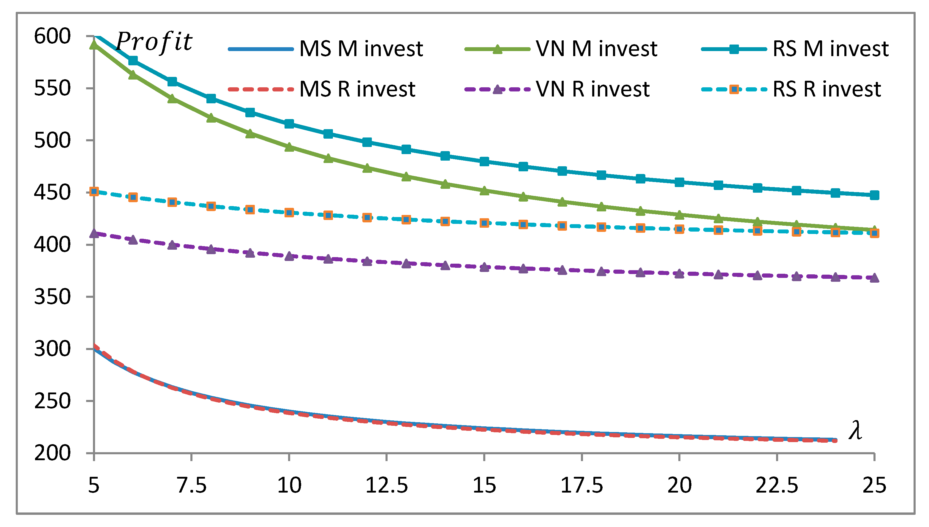
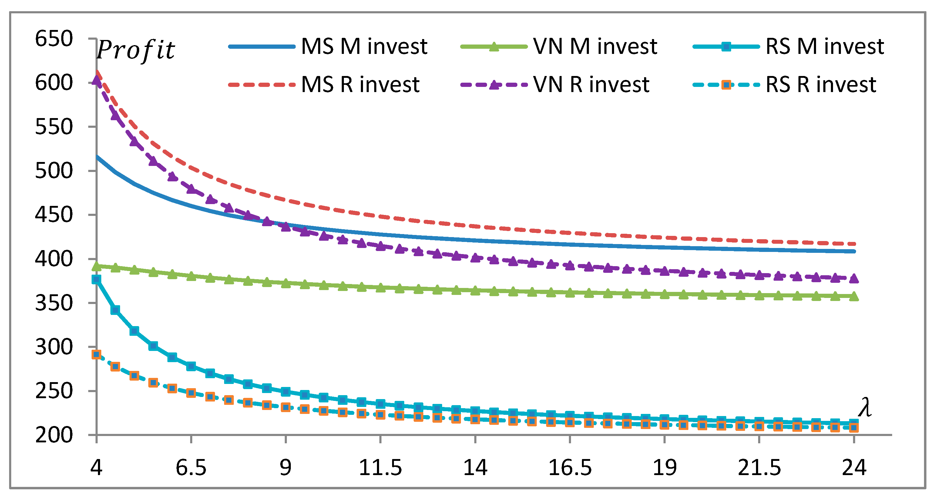
In order to illustrate the results more intuitively among different cases, we present a numerical example. More specifically, we discuss the impact of investment factor (i.e., $\lambda$) on the optimal profits of both firms. In this example, we set $\alpha =100$, $\beta =3$, $\gamma =3.5$ $c=1$, $t=0.4$, and we let $\lambda$ vary from 4 to 24. These parameters satisfy the constraints we assumed in the model setting. In Figure 1, we depict the retailer’s optimal profits in three types of power structures, with different sustainable investors, respectively. Correspondingly, the manufacturer’s optimal profits are represented in Figure 2.

The numerical example confirms results presented in Corollaries 1 and 2 and Proposition 3. It is interesting to notice that both firms’ optimal profits decrease in investment factor, even if they are not responsible for the sustainable investment. Since demand increases after sustainable investment, both firms have incentive to raise price. As a result, the benefit from investment cannot cover the additional cost or demand lost due to incremental price. Furthermore, the gap between scenarios of different investors narrows as the investment factor increases.

Then, comparing the optimal sustainable effort differentiated by investors in the supply chain in three types of structure, we have the following proposition.

Proposition 4.

1.

In the MS power structure, the manufacturer’s sustainable investment is higher than the retailer’s (i.e., $e_m^m>e_m^r$) if $\gamma <\widehat{\gamma }$, while the retailer makes higher investment (i.e., $e_m^r\ge e_m^m$if $\gamma \ge \widehat{\gamma }$. Here, $\widehat{\gamma }$ is obtained by solving the following equation: $8t\lambda {\beta }^2-\gamma {\left(\gamma +t\beta \right)}^2=0.$

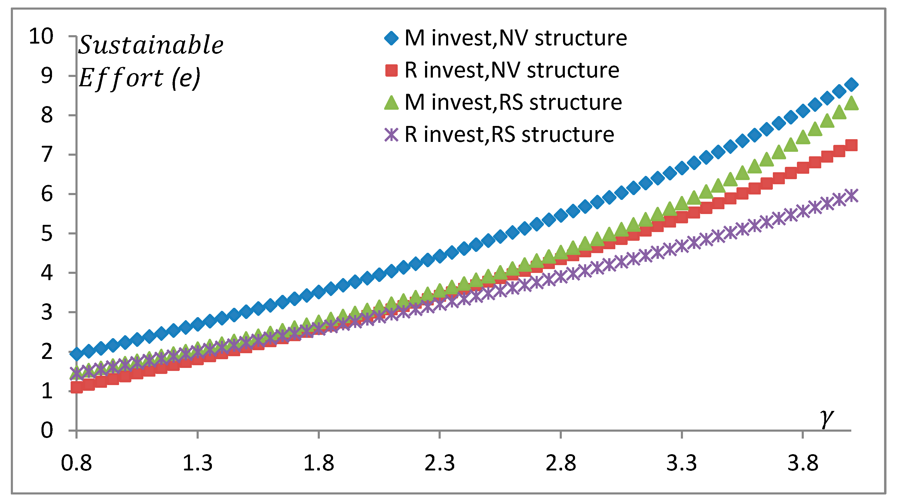
2.

In the VN power structure, the manufacturer’s sustainable investment is higher than the retailer’s (i.e., $e_n^m>e_n^r$);

3.

In the RS power structure, the manufacturer’s sustainable investment is higher than the retailer’s (i.e., $e_r^m>e_r^r$).

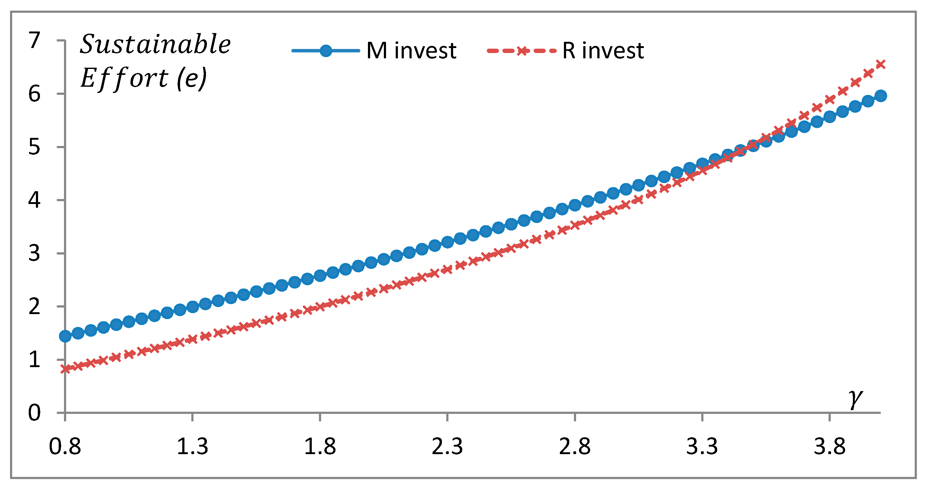
This proposition implies that under either VN or RS supply chain structure, the optimal amount of sustainable investment in the manufacturer investment case is higher than that in the retailer investment case. However, in the MS structure, the retailer is willing to make more investment than the manufacturer does, if the sustainable sensitivity of demand is relatively high. It hints that, in most of cases, it is more beneficial from an environmental perspective that the manufacturer plays the role as sustainable investor.

We examine the impact of sustainable sensitivity of demand (i.e., $\gamma$) on the optimal sustainable effort of both firms. We set $\alpha =100$, $\beta =3$, $\lambda =4$ $c=1$, $t=0.2$, and we let ³ vary from 0.8 to 4. The parameters satisfy the constraints we assumed in the model setting. In Figure 3, we depict the sustainable effort in MS power structure. Sustainable effort in VN and RS power structures is shown in Figure 4.

Both figures further confirm the Proposition 4 that manufacturer’s sustainable investment benefits the environment for most cases. It can be explained by the fact that the manufacturer has additional incentive for sustainable investment from tax saving. Moreover, in the VN and RS power structures, the gap widens as the sustainable demand sensitive factor increases. It means that the manufacturer is increasingly motivated to make sustainable effort when the sustainable sensitivity is high.

7. Conclusions and Future Research

In this paper, we develop an analytical model to study a two-echelon sustainable supply chain consisting of one retailer and one manufacturer with three different power structures. Besides retail and wholesale price decisions, both the apparel retailer and manufacturer have options to make sustainable investment represented by sustainable effort. To model the incentive of sustainable investment, we consider that a greater sustainable effort investment reduces the environmental tax and increases the market demand. We consider two investment modes offered by the manufacturer and the retailer, respectively. Both supply chain members pursue maximizing their profits. The optimal operational decisions are derived and compared. The main findings are as follows.

From an economical perspective, the more power a fashion retailer (manufacturer) has over her (his) supply chain partner, the more economic benefit can be gained for the powerful supply chain member. They often utilize their power to charge a higher retail price or wholesale price rather than make more sustainable effort. This result holds regardless of which party makes the sustainable investment, unless the sustainable sensitivity of demand is relatively low, and then the retailer’s investment increases in her power.

From an environmental perspective, the VN model generates the highest sustainable investment when the manufacturer invests in sustainable effort. In addition, this result also holds in the retailer’s investment case, when the sustainable sensitivity of demand is relatively high. However, we also notice that there are two pure strategy equilibriums, in which one of the supply chain members invests, in the VN model. Different pure strategy equilibrium is preferred by each firm. That is, each one waits for the other to invest. Interestingly, when a firm becomes less powerful in the supply chain, she/he has more incentive to make sustainable investment. It is more notable for the manufacturer because he has additional benefits from environmental tax reduction. Moreover, manufacturer’s optimal sustainable investment is higher than the retailer’s in most cases, except for the MS model with relatively high sustainable sensitivity of demand.

This paper is an early attempt to understand the economic and environmental performance of sustainable investment from different supply chain members in different power structures. The present model has its own limitations that also point toward potential future research directions. Firstly, the demand is deterministic and depends on the retail price and sustainable effort in our model. This setting does not consider the randomness of demand in reality, though it provides neat and tractable results. Hence, one future extension is to investigate a research problem using stochastic demand models. In addition, we attempt to further investigate a research problem by considering a scenario in which both members of the supply chain make sustainable investment, and then study the supply chain coordination with different contracts. Finally, our model considered the two-echelon supply chain consisting of a retailer and a manufacturer. In the real world, fashion supply chains are often much more complicated. It is interesting to consider multi-retailer and/or multi-manufacturer structures and explore how the spillover effect influences the sustainable investment.