1. Introduction
Water, energy, and food (WEF) are strongly interconnected: each depends on the other for a lot of aspects, spanning from guaranteeing access to services to environmental, social, and ethical impact issues, as well as economic relations.
The development, use, waste, and pollution generated by demand for these resources drive global changes and create concerns for resource scarcity and quality. To date, a new approach to the concept of sustainable development is emerging, and a joint analysis of these three areas is needed. “Demand for water, food and energy is expected to rise by 30–50% in the next two decades, while economic disparities incentivize short-term responses in production and consumption that undermine long-term sustainability. Shortages could cause social and political instability, geopolitical conflict and irreparable environmental damages. Any strategy that focuses on one part of the WEF relationship without considering its interconnections risks serious unintended consequences” [
1].
The analysis of the nexus has to be placed into a framework of policy decisions. Indeed, while it is well established that water, energy, and food are three crucial sectors for promoting sustainable growth, a lot has to be done to practically implement the WEF nexus. In particular, one specific issue is related to the pricing and government policies responsible for setting measures such as taxes and subsidies that deeply influence political economies. While these measures have been heavily used in the food sector, wherein prices are actually determined by policy interventions both in developed and developing countries [
2,
3], the impact of these policy interventions on water resources in terms of ecosystem costs, over-use, and pollution have been almost ignored. Conversely, water analysis is of the utmost relevance given its limited substitutability and its essential prominence in terms of human life. The issue of pollution and quality make water more critical than food and energy and underline the need for a deeper focus within the nexus [
4,
5].
In the last years international organizations have organized several conferences to raise awareness of the WEF nexus [
6], and some studies have addressed this issue by trying to provide a theoretically integrated view aimed at understanding how to tackle these complex relationships when designing policies and taking appropriate actions [
7,
8,
9,
10]. These studies have analyzed the technical connection that exists between the three elements in order to highlight the need for a joint policy aimed at ensuring sustainable development.
From an economic point of view, there are still very few analyses that utilize empirical approaches to validate the recent theoretical literature [
11,
12,
13,
14]. This area of study is clearly wide, and an economic analysis of the link aimed at understanding the interactions and correlations on a global scale is still needed.
Within this framework, the aim of our paper is to empirically analyze the market integration through the study of volatility spillovers and the correlation between indexes representing the economic component of the WEF nexus. Indeed, the economic theory states that the more the economic components are correlated, the greater is the possibility that shocks propagate between sectors. Therefore, taking the economics perspective has the important advantage of highlighting the strength of these relations and their dynamics to better understand if and how shocks are transmitted from one sector to the others.
To perform the analysis, we use a multivariate GARCH model with dynamic conditional correlation [
15], which appears to be the most proper econometric methodology to study the shock transmissions, the volatility spillover effects, and the dynamics of conditional volatility between series.
The water sector is investigated using equity indexes that represent the performance of the industry involved in water business both at global and continental levels such as Europe, North America, Latin America, and Asia. For the food and energy sectors, we use two sub-indexes of the S&P GS-Commodity Index; respectively the S&P Agriculture-Livestock Index and the S&P Energy Index. We use daily data spanning from November 2001 to May 2013. The timeframe covers the 2008 economic and financial crisis and allows us to assess whether it influenced the relationship between the sectors.
The novelty in this work is threefold. Firstly, the paper focuses on a topic of great relevance from an economic, environmental, and ethical perspective, as recently outlined by many international organizations. The complex interactions and policy implications that consider all three sectors together need more work in order to effectively support decision-making. To the authors’ knowledge no previous study has investigated market integration between WEF with the aim to understand economic spillover between the three sectors. Secondly, it performs the first econometric analysis of the financial relationship among these three sectors using a Dynamic Conditional Correlation model that permits the evolution of the relationships of the index to be studied in a dynamic framework and the times of high and low correlation between the sectors to be detected. A good understanding of the origins and drivers of local volatility and cross market correlation is crucial because it can help policy makers in taking the proper measures to mitigate the potential correlations across the use of these resources, which may create future undesirable shocks to the world and the domestic economy. Third, from a geographical perspective, the analysis covers both global and local markets. Indeed, taking into account that water, energy, and food are inextricably interlinked around the world, the nexus approach needs to be addressed on a global scale, but at the same time we also know that actions must be local. Therefore, considering that different areas in the world have different degrees of financial integration, we focus both on a global scale and on different geographical areas such as Europe, North America, Latin America, and Asia.
The paper is organized as follows:
Section 1 focuses on issues related to the technical nexus,
Section 2 presents the data and the method,
Section 3 reports the results, and
Section 4 discusses the main conclusions.
The Water-Energy-Food and Nexus
Population growth, changes in lifestyles, and increasing prosperity are putting rising pressures on resources. According to international organizations [
16], by 2030 the demand for food, energy, and water is expected to rise by 30–50%.
Resources are scarce, and shortages could impact on communities and cause social and political instability, geopolitical conflict, and environmental degradation. Consequently, in order to satisfy such an increasing demand, many efficiency improvements for both development and implementation need to be achieved such as new sources for food, changes in water use, and a more efficient mix of energy production systems.
Improvements require not only research and the development investments and funds but also an integrated approach since WEF are strongly interrelated. Indeed, agriculture and food both require large amounts of water and energy in all stages of production; energy production needs water as well as bio-resources; water extraction and distribution requires energy. Researchers [
7] clearly and exhaustively identify the descriptive elements of the WEF nexus. Specifically, many billions of people are without access to any or all the three areas (quantity or quality or both; lack of access to modern fuels or technologies for cooking/heating; lack of access to safe water; no improved sanitation; people chronically hungry due to extreme poverty; lack of food security). Additionally, all three areas have rapidly growing global demand, and all have resource constraints. Finally, they all have different regional availability and variations in supply and demand, and all have strong interdependencies with climate change and the environment.
Given those interrelations, any improvement strategy that focuses on water, food, and energy without considering their nexus risks unintended negative consequences [
17]. For example, the use of biofuel reduces vehicle emissions, but, at the same time, it may impact the worldwide availability of food and land [
18] and lead to higher agricultural prices [
19,
20]. Likewise, shale gas extraction can reduce the use of fossil fuels and is cleaner-burning than oil and coal; nevertheless, hydraulic fracturing requires large amounts of water, and this reduces the availability of water for other uses. Moreover, the fluid injected into the subsurface contains chemical additives that can contaminate surrounding areas. Furthermore, the development of irrigated agriculture has boosted agricultural yields and contributed to price stability and thus to poverty reduction [
21]. Those are clearly trade-offs that policy makers have to think about when assessing planning for investments, actions, and policies.
Recent studies have provided only a few attempts at frameworks aimed at analyzing the combined effects of the agriculture, energy, and water sectors from an economic perspective and on a global scale. Generally this topic was analyzed in the literature following different approaches, technical or economic, and different fields of application such as agricultural-water and energy-water, either separately or jointly.
The technical approach has been addressed more often to analyze the relationship between energy and water. Studies mainly focus on energy consumption and water use, applying life-cycle evaluation or numerical simulation [
22,
23,
24]. The most recent papers focusing on the water-energy nexus [
25,
26] use input-output tables to describe the supply consumption relationship between water supply and primary energy sectors. One study [
27] found that gradually eliminating conventional power generation units, which are the most water-intensive, can significantly reduce water needs by the application and effective operation of methods and projects, which improve not only the supply but also the demand for water.
Works considering jointly water, energy, and agriculture are less common [
7,
8,
9,
28]. These studies analyze the technical connection that exists between the three elements in order to highlight the need for a joint policy aimed at ensuring sustainable development.
Conversely, studies following a strictly economic approach focus only on pairs of relationships separately, i.e., water-agriculture or water-energy. As far as water and agriculture, few studies deal with the effect of agricultural prices on water demand and management [
29,
30,
31,
32,
33].
The economic relationship between water and energy that directly focuses on the impact of energy prices on the water sector is investigated in only two studies [
34,
35]. They find that rising energy prices increase costs for water extraction and conveyance, thus altering water allocation and distribution. The development of technologies to extract water more cheaply and transport water more efficiently can offset the effects of rising energy prices, which are expected to induce the adoption of new and better technologies.
Thus, the water, food, and energy nexus still needs very thorough analysis, global governance, and integrated response strategies.
2. Data and Methods
2.1. The Dynamic Conditional Correlation Approach
In order to allow for interdependencies of volatilities across WEF markets, we apply a multivariate GARCH (M-GARCH) model with the conditional variance assumed to be Vector Autoregressive Moving Average (VARMA) [
36] and with the dynamic conditional correlation (DCC) specification of [
15] for the analysis of dynamic covariances and correlation across markets. This approach has been shown to be more useful when studying volatility spillover mechanisms than univariate models that do not allow for a cross-market volatility spillover effect, which is likely to occur with increasing market integration. One of the main advantages of this model is that it permits the exploration of the shock transmissions between water, energy, and food, the volatility spillover effects, and the dynamics of conditional volatility between the three series. Moreover this model provides meaningful estimates of the unknown parameters with less computational complication than other multivariate specifications [
37].
In the MGARCH approach, we model the mean equation, the variance equation, and the time relationships as follows.
We use a Vector Autoregressive (VAR) system in the mean equation to allow for autocorrelation and cross correlation in the returns for the three variables (WEF). To let a shock in one of the three variables affect the variance of the others in the system, we modeled the variance equation to be vector autoregressive moving average-GARCH [
36]. Finally, to increase the model flexibility for studying the evolution of the relationships of the variables over time, we used the dynamic conditional correlation (DCC) model of [
15].
In the multivariate GARCH, we use the following mean equation specification:
where:
i is index of the investigated sectors,
n is the total number of sectors (in this work
n = 3 for water, energy, and food),
Ri,t is the return calculated by first log difference of
ith price index at time
t,
ci is scalar depending on the
i sectors,
mij represents coefficients that measure the relationship between current period returns and last period returns,
εi,t is a random error term of the mean equation with conditional variance
hi,t, and
vi,t is the innovation and is independent and identically distributed (i.i.d), which is a random vector independent and identically distributed where each random variable has the same probability distribution as the others and all are mutually independent.
Information criteria are used for the lag length selection for VAR in the mean equation. Based on Akaike information criterion (AIC), Schwarz-Bayes information criteria (SBC), and Hanan-Quinn information criteria (HQ), in all the models tested the number of lags selected for the VAR systems is equal to one.
The variance term is specified as follows [
36]:
Equation (3) is a generalization of the specification in [
37], which accommodates the interdependencies of volatility across variables.
hi,t is the conditional variance at time t;
hj,t−1 represents the past variance when
j =
i, while, when
j ≠
i, it denotes the past conditional variance of the variables in the system.
αii represents the conditional ARCH effect, which is the measure of short-term persistence, whereas αij represents cross conditional ARCH effects. βii expresses the sensitivity to past volatility in the long run (GARCH effect), and βij denotes long-run volatility interdependency.
The analysis of dynamic covariances and correlation across markets is carried out using the dynamic conditional correlation (DCC) by Engle [
15], which is a generalized version of the constant conditional correlation (CCC) model by [
38]. This representation is one of the most widely used in financial analysis [
39,
40] and, more recently, in energy finance [
41,
42,
43].
The specification of Engle’s DCC model is as follows:
where H
t is the conditional covariance matrix, D
t is a n × n diagonal matrix of conditional, time varying, standardized residuals estimated in a first step by univariate GARCH models, and R
t is the n × n time varying correlation matrix with the following form:
Conditionally to the estimated
Dt, the correlation component
Qt, which is a weighted average of a positive definite and a positive semidefinite matrix, is estimated in a second step with the following equation:
where
Q0 is the unconditional correlation matrix of the standardized residual epsilon and
θ1 and
θ2 are the parameters that respectively indicate the impact of past shocks on current conditional correlation and the impact of the past correlations. The model is mean reverting as long as
θ1 +
θ2 < 1. The dynamic conditional correlation coefficient
ρI,j,t, which is a typical element of
Qt, is calculated as in Equation (7):
In the empirical application, the model is estimated using a Quasi Maximum Likelihood Estimator (QMLE) by the Broyden–Fletcher–Goldfarb–Shanno (BFGS) algorithm. t statistics are calculated using a robust estimate of the covariance matrix.
For the specific purpose of this study we specify a M-GARCH with n = 3, given the three variables water, energy, and food.
2.2. Data
We use daily data spanning from November 2001 to May 2013 obtained from Datastream, a Thomson Reuter dataset. For the water component, we use the Water Index composed of 23 liquid and tradable stocks from companies operating in water businesses around the world. The companies included in the indexes are: VEOLIA ENVIRONNEMENT F:VIE 15Y Euronext.liffe Paris, AMERICAN WATER WORKS U:AWK 8Y NYSE United States, UNITED UTILITIES GROUP UU. 26Y London United Kingdom, SEVERN TRENT SVT 26Y London United Kingdom, SUEZ F:SEV 7Y Euronext.liffe Paris, GUANGDONG INVESTMENT K:GUAN 28Y Hong Kong Hong Kong, PENNON GROUP PNN 26Y London United Kingdom, AQUA AMERICA U:WTR 43Y NYSE United States, BEIJING ENTS.WATER GROUP K:WANO 23Y Hong Kong, CPAD.SANMT.BASICO DE SAOP.ON BR:SAB 19Y Sao Paulo Brazil, AGUAS ANDINAS CL:EMO 26Y Santiago Chile, METRO PACIFIC INVS. PH:MPI 9Y Philippines, GELSENWASSER D:WWG 43Y Deutsche Boerse AG, INVERSIONES AGUAS METROPOLITANAS CL:IAM 10Y Santiago Chile, ATH.WT.SUPPLY & SEWAGE G:EYD 16Y Athens Greece, CHINA EVERBRIGHT WATER T:BIOT 12Y Singapore, CITIC ENVIROTECH T:UENV 12Y Singapore, MANILA WATER PH:MWC 11Y Philippines, SEMBCORP SALALAH POWER OM:SSP 2Y Muscat Securities Market Oman, SIIC ENVIRONMENT HDG. T: ASWT 11Y Singapore Catalist Singapore, SHARQIYAH DESALINATION OM:SDC 2Y Muscat Securities Market Oman, TALLINNA VESI EO:TVE 11Y NASDAQ OMX Tallinn Estonia, THESSALONIKI WATER SUPP. G:EYAP 14Y Athens Greece.
The constituents involved are distributed between water utilities and infrastructure (water supply, water utilities, wastewater treatment, water purification, water well drilling, water testing, and water sewer and pipeline construction) and water equipment and materials (water treatment chemicals, water treatment appliances, pumps and pumping equipment, plumping pipes, fluid power pumps and motors, fluid meters, and counting devices). The index consists of companies that represent 75% to 80% of the market capitalization. We also use continental sub-indexes for Europe, North America, Latin America, and Asia, representing the performance of the major industry involved to water sector for a given area. For the agriculture and energy sectors we used two sub-indexes of the S&P GS-Commodity Index. Specifically the indexes are a proxy for the level of nearby commodity prices for agriculture-livestock and energy. Both the indexes are calculated primarily on a world production weighted basis and comprise the principal physical commodities that are the subject of active, liquid futures markets. The weight of each commodity in the index is determined by the average quantity of production as per the last five years of available data. The rationale for the choice of these two latest variables is that these commodity indexes have gained increasing importance within financial markets according to commodity index traders and therefore can be viewed as a financial asset that can be appropriately analyzed to investigate market integration with the water sector [
44].
Indeed, water, energy, and food indexes constitute a benchmark for a large amount of financial products with a real-asset exposure; namely, the commodity index swaps, exchange traded funds (ETFs), and exchange traded notes (ETNs). Typically, hedge funds, pension funds, and other large institutions purchase these financial instruments with the aim of diversifying their portfolios [
45].
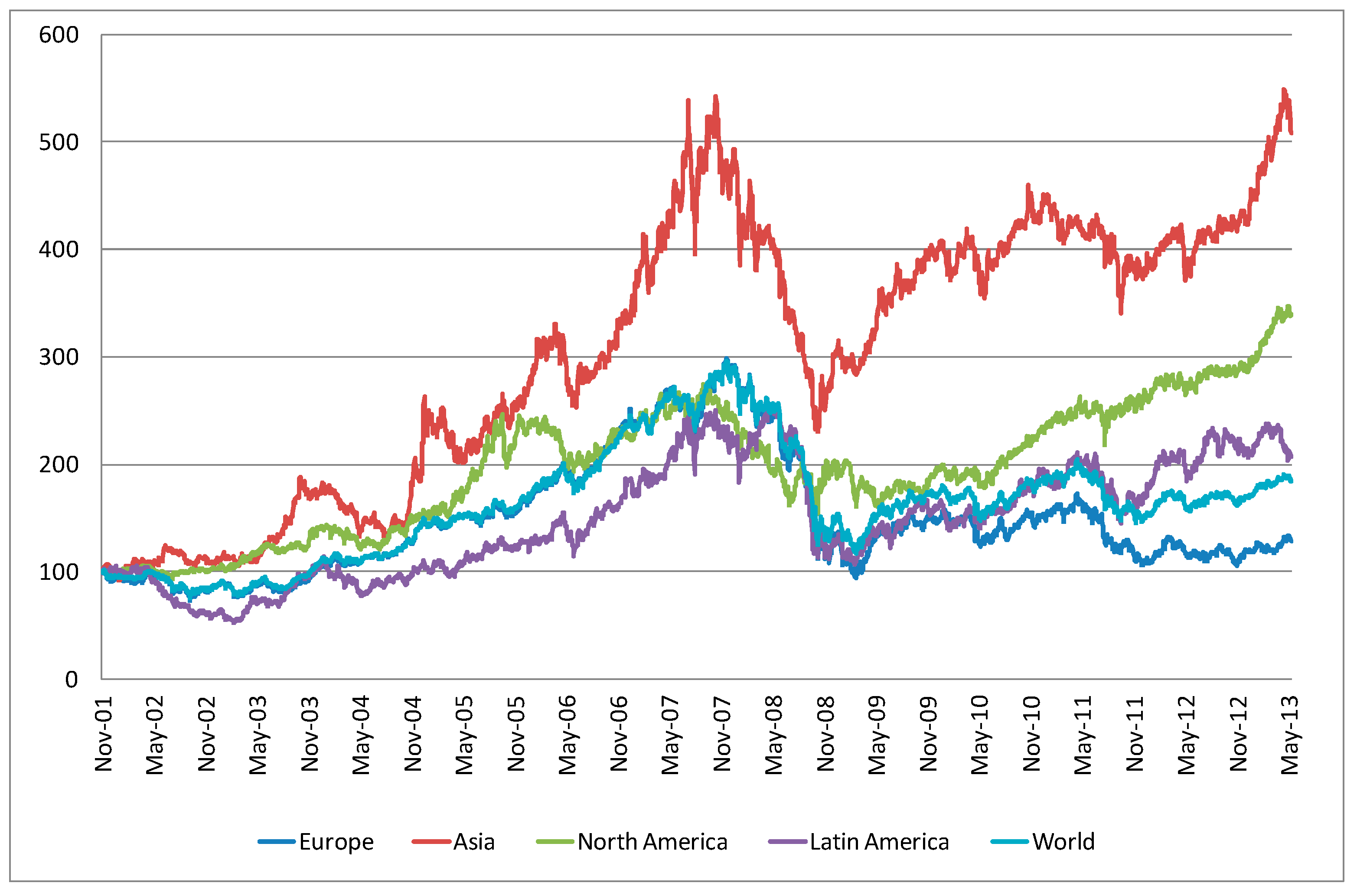
Figure 1 shows the trend for the water index for the world and for the other four areas considered. All the series show an increasing trend until the end of 2007, which then decreased to be followed by a new growth, but distinct differences are present between the areas.
The Asia index more than quintupled during the first six years, but then its value dropped during the financial crisis. Afterwards the index grew again very intensely until it reaches the 2007 level. Energy and agriculture follow similar trends although they have become fairly distinguished in recent years. The North America water index increases considerably crisis, whereas the Europe index shows poor performances after 2011.
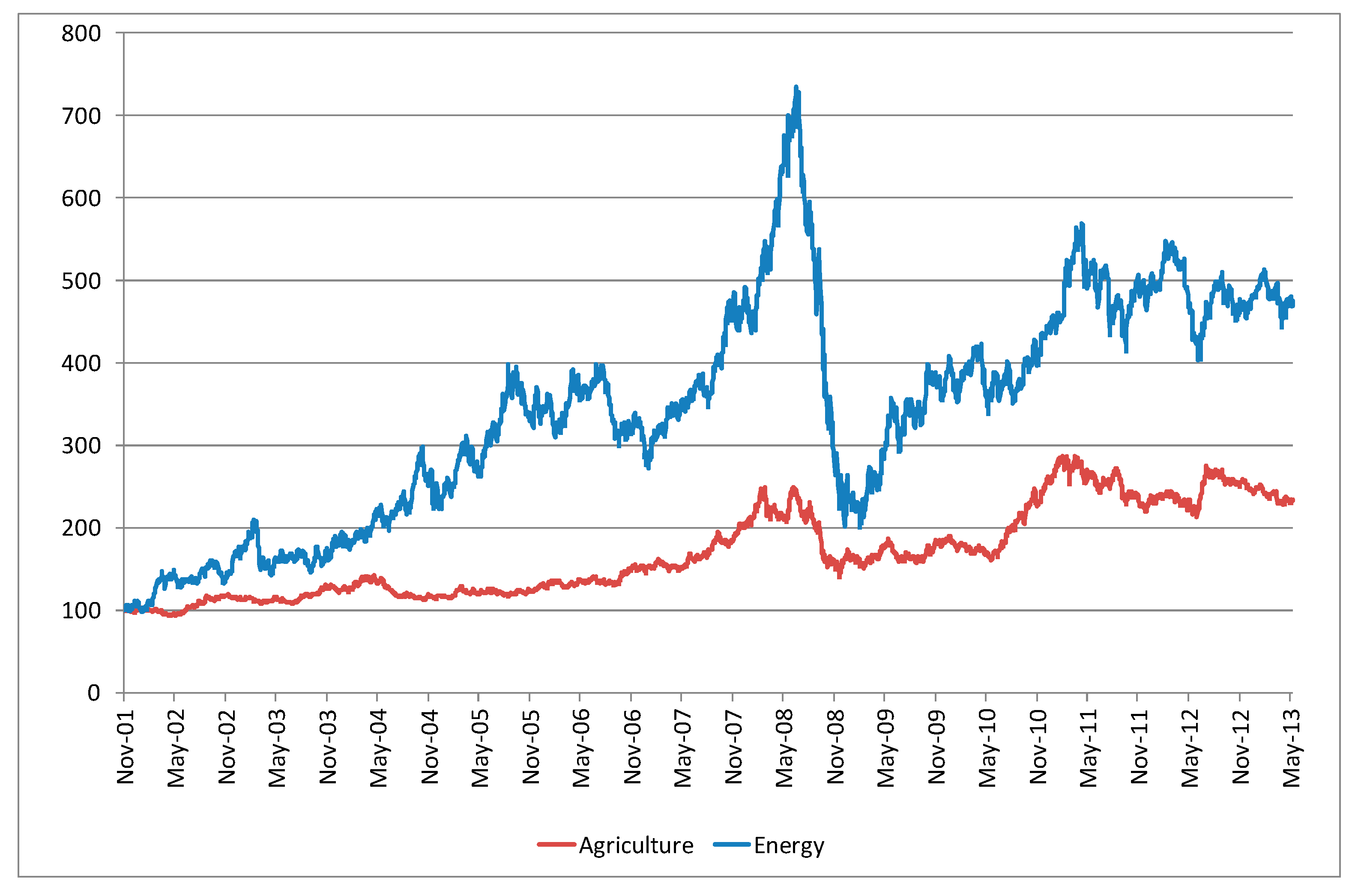
Figure 2 reports the trends of the agriculture and energy indexes. The graphical representation suggests that the two series follow an increasing trend until the crisis, both reaching unprecedented heights in the middle of 2008 and subsequently still declining with remarkable speed. After this period, the indexes level grew again at different rates, but only the agricultural index has reached and exceeded past levels.
Table 1 shows the descriptive statistics of continuously compounded daily returns for each series. Many of the indicators suggest that the series are heteroskedastic and therefore need to be treated with an Autoregressive Conditionally Heteroscedastic-Generalized Autoregressive Conditional Heteroscedastic (ARCH-GARCH) approach. From the daily standard deviation, we see that the level of volatility is generally high enough: the energy price index return is the most volatile and the agriculture price index return the least volatile.
Noticeably, the water index returns display a stronger amount of kurtosis than the agricultural and energy indexes. Skewness is negative for all the indexes but Asia. The higher the kurtosis coefficient is above the normal level, the more likely it is that future returns will be either extremely large or extremely small. This fact suggests the need to account for the presence of volatility in our models, confirming the idea of using an ARCH approach.
3. Results and Discussion
We first test for the existence of ARCH effects in the series, and then we proceed with the estimate of a multivariate GARCH model, with the mean equation modeled as a VAR system.
Table 2 reports results of the multivariate GARCH estimate for all the investigated areas, and the diagnostic tests are reported in
Table 3. The estimates of these models can provide measures of the significance of the short-run persistence, the ARCH effects of past shocks, the (
αi,i) and the (
αi,j) between sectors, the long-run persistence, the GARCH effects of (
βi,i) and spillover (
βi,j), and past volatilities. In the table, the coefficient
α1,3 represents the short term volatility spillover from energy (3) to water (1), while
β2,3 represents the long term volatility spillover from energy (3) to agriculture (2).
The first part of the table shows the mean equations estimates and the second the variance equation estimates. Overall, most of the coefficients are significant for the world and for the other geographic areas. In the following, we will focus our discussion only on the significant terms.
In the variance equation, the ARCH effects are mostly significant. The conditional effects (αi,i) are always positive and bigger than the cross effects, as expected, with the water coefficient (ranging from 0.055 to 0.074) showing the strongest shock dependence. The agriculture and energy markets highlight a smaller dependence (from 0.035 to 0.042) and a very similar news sensitivity between areas.
The inter-sector short run/shock spillovers of the three indexes show different patterns between geographical areas and between each other. The agriculture to water coefficient (α1,2) is significant only in the world equation, whereas no substantial effect is present at the local level. Positive spillover effects are present in particular in North and Latin America. It is interesting to note that shocks from water to agriculture and from agriculture to energy are always negative, suggesting that water volatility tones down agricultural volatility and then energy volatility.
Examining market interactions in terms of the conditional second moment can provide better insight into the dynamic price relationships of markets. Long term persistence expressed by GARCH coefficients (βii) is still always present, with all the coefficients being significant. For each i, the estimated bii values are bigger than their respective estimated αii values, ranging from 0.802 to 0.957. This suggests that past volatilities are more important in predicting future volatility than past shocks or news in all three sectors. There is also evidence of cross volatility effects between all three sectors, with many αij coefficients being significant at the 1% or 10% level. Additionally, in this case, the world and the Americas show the best performance in statistical terms.
Specifically, cross volatility in water-agriculture is always positive in both directions of causality except for Asia. Instead water-energy links show negative cross-GARCH coefficients, implying therefore a volatility cooling effect between these sectors. Although this concerns the movement from agriculture to energy and vice versa, the results still show past volatility spillovers for the most of the areas. Specifically there is a negative cross-volatility from energy to agriculture and from energy to water, although there is also a volatility cooling effect from water to energy.
Table 3 reports the diagnostic tests
Q(12) and
Q(20) for the presence of autocorrelation in squared residuals.
The results confirm that the models perform statistically well. The ARCH and GARCH coefficients highlight that volatility spillover exists between the water, agricultural, and energy sectors; this result is relevant since it confirms the existence of a nexus in the short and long term.
Nevertheless
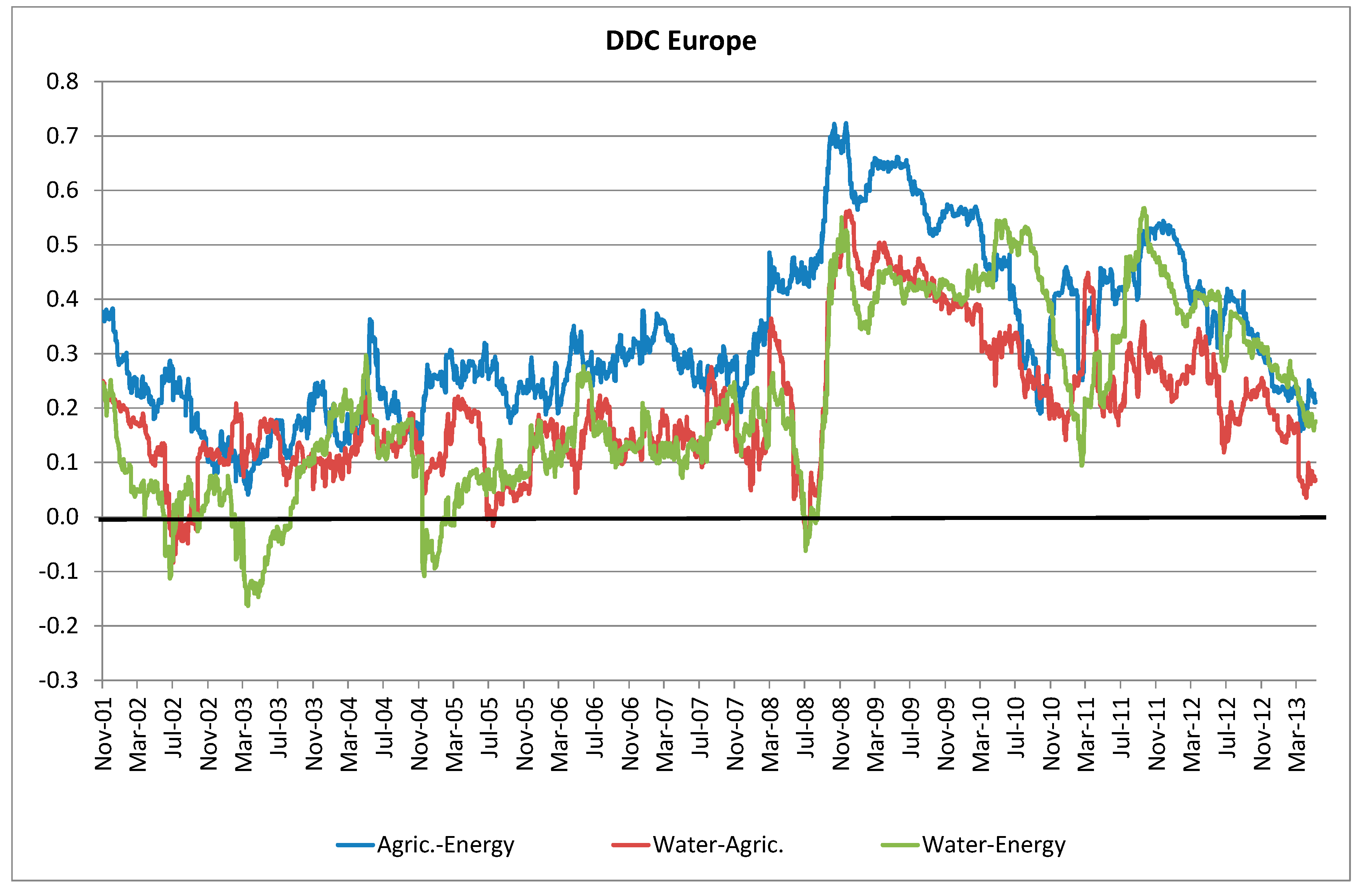
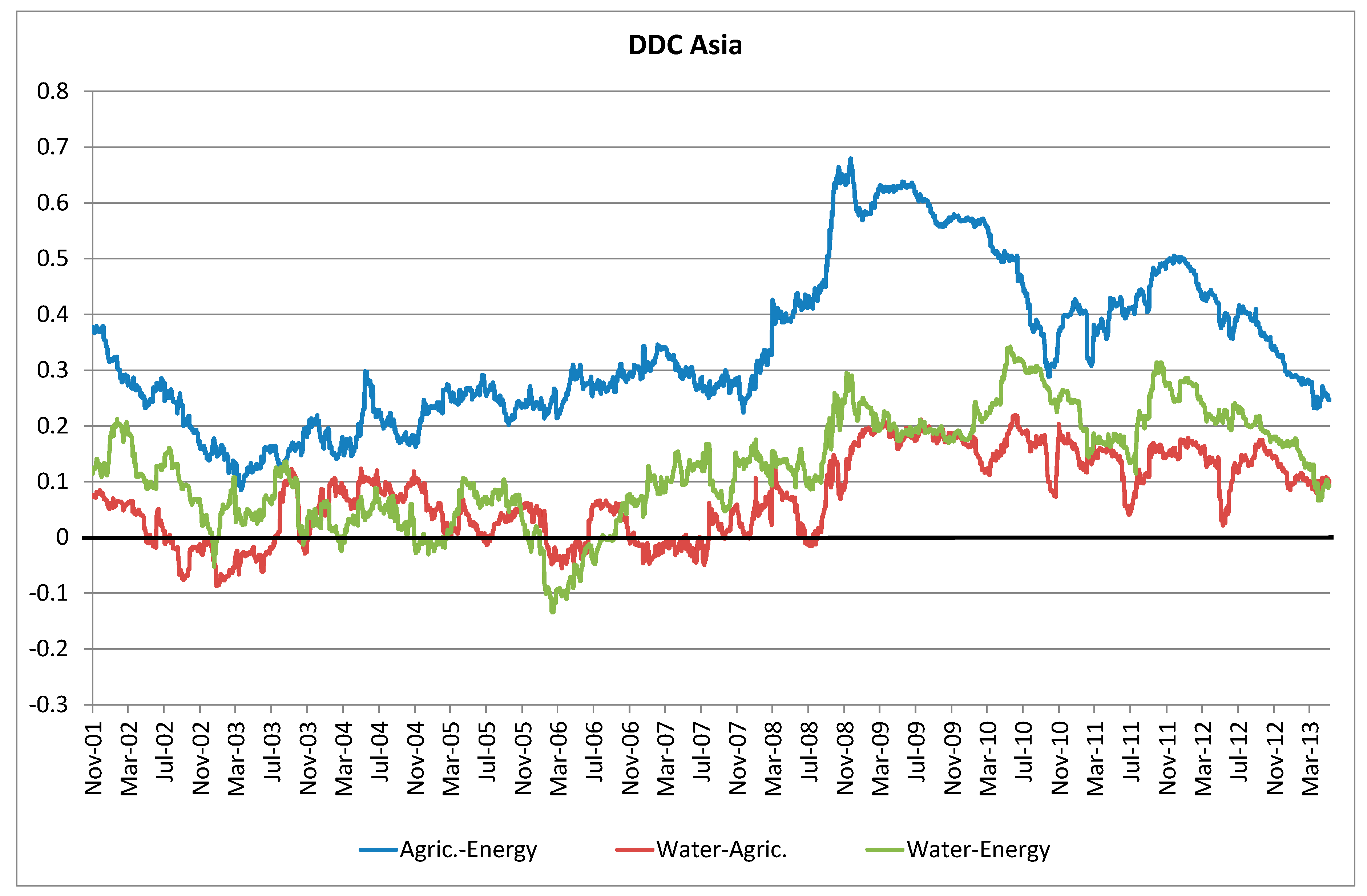
Table 2 reports results considering a very long period, which includes numerous events and circumstances. To better fit with the purpose of this analysis, we also report the graphs of the time varying dynamic conditional correlations (
Figure 3,
Figure 4,
Figure 5 and
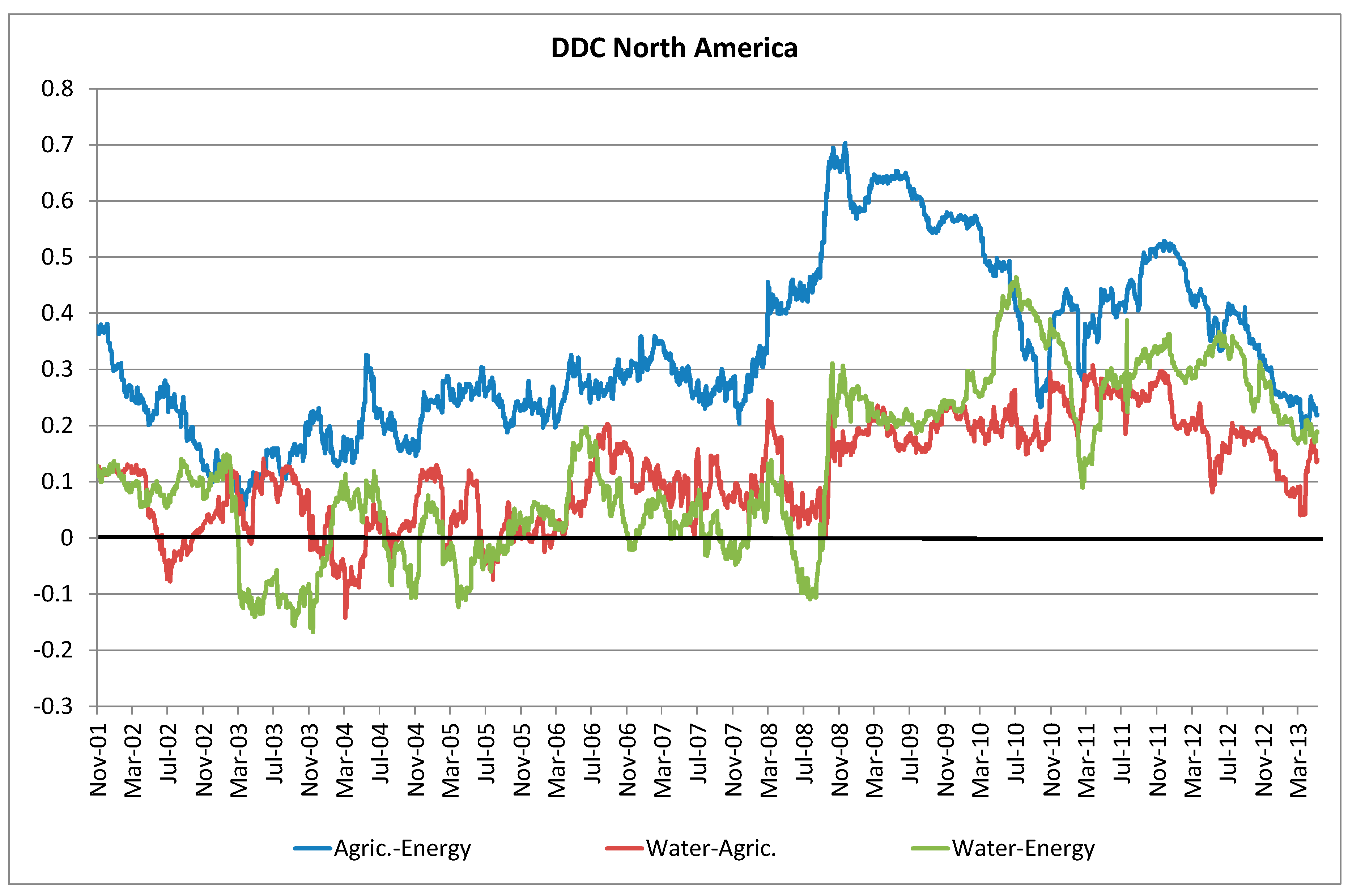
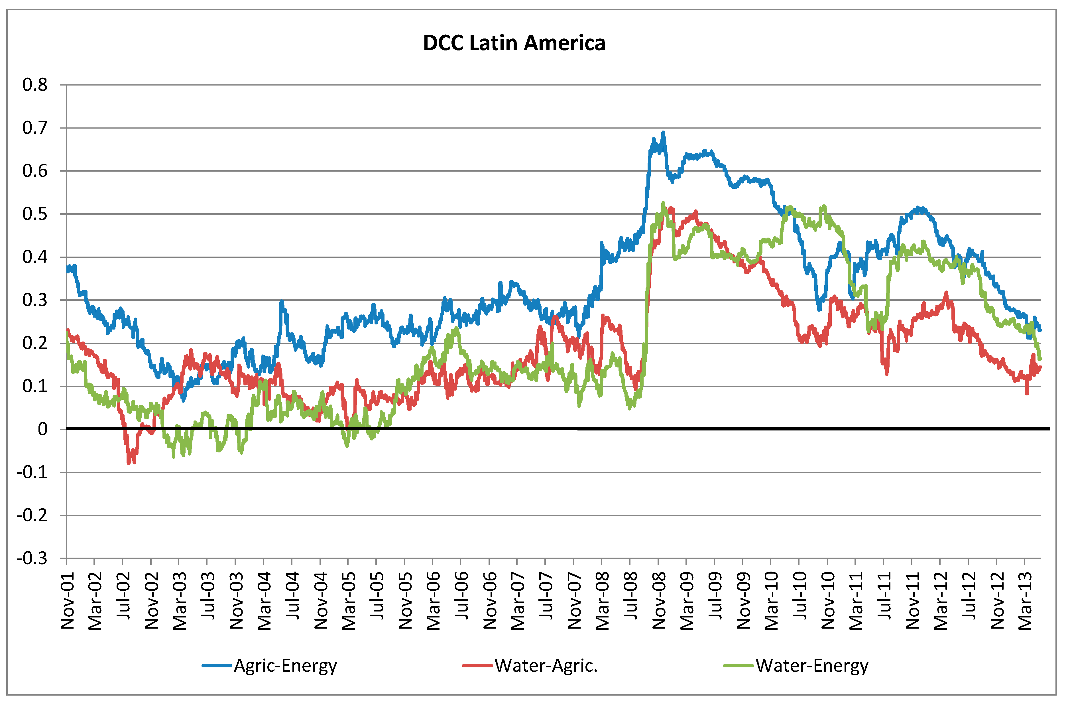
Figure 6) that plot the time series for each of the geographical areas studied for the following pairs of series: agriculture/energy, water/agriculture, and water/energy.
These figures show how the effects evolve over time and the relationship between price indexes as functions of both the history of variance (volatility) that each series has undergone and the correlation between them. Overall, the dynamic conditional correlation is positive. A very strong break is evident in the middle of 2008, when the economic and financial crisis occurred. After this moment, a strong upwards pattern is evident for each pair of correlations and for all the geographical areas.
The relationship between agriculture and energy evolves with a similar pattern among the different areas investigated and shows the highest levels of correlation in Asia and North America (
Figure 4 and
Figure 5).
The dynamics of the water-energy and water-agriculture correlations show similar trends too, highlighting the effect of the crisis on the volatility transmission. Specifically water and energy show very similar dynamics between Europe and Latin America (
Figure 3 and
Figure 6) and between North America and Asia. A similar distinction is outlined by the dynamic conditional correlation between water and agriculture. In Europe and Latin America, both the DCCs sharply increased after the global economic downturn exceeding level 0.5, whereas this evidence becomes less noticeable in North America and Asia, where correlations reach level around 0.3 and 0.2, respectively.
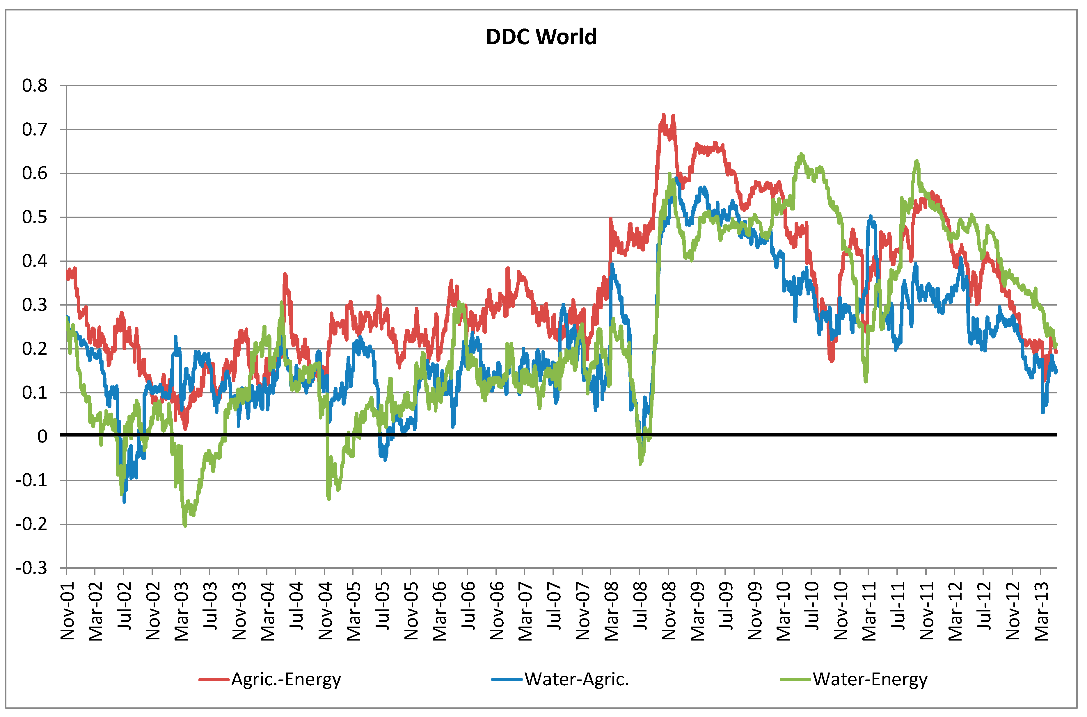
When analyzing the world as a whole (
Figure 7), the differences in the lines that show the DCCs are much less, and this strengthens the idea that the water issue is much more substantial in a global perspective. After the crisis, a strong upwards pattern is evident for each pair of correlations. Specifically, in few weeks, the conditional correlation between water and energy jumps from −0.06 up to 0.60; similarly, the conditional correlation between water and agriculture increases from −0.03 to 0.59.
Interestingly, before the financial crisis, the correlation between agriculture and energy was always stronger than the correlation of the two variables with water. Moreover, the water and energy relationship shows negative values only in a few short windows. Conversely, after the global economic downturn, this evidence becomes unclear; in particular, in some periods the dynamic conditional correlation between water and energy is higher than the correlation between agriculture and energy. This highlights the rising relevance of water issues within the nexus.
In
Figure 8 we synthesize all the previous information by constructing a graph that tries to express for each geographical area the nexus between water, energy, and food. Specifically, for the investigated area, the graph describes a weighted mean value of the three dynamic conditional correlations (agriculture-energy, water-agriculture, and water-energy).
During the first period analyzed, from the end of November 2001 until September 2008, the nexus between water, agriculture, and energy moves on the same level for all the investigated areas with the DCC ranging from −0.02 to 0.38 and 0.16; in the subsequent period, all the values more than doubled reaching peaks greater than 0.6. In this case, the world line also almost always shows the highest correlations. These results are in line with the recent economic literature [
46,
47,
48,
49] that provides evidence that the commodity returns and stock returns correlation has gone up substantially during the recent financial crisis, despite the traditional negative correlation between commodity and equity returns documented by [
50,
51,
52].
The huge amount of money invested by index traders in commodity markets, especially during and after the 2008 financial crisis, has created a new link between commodities and stock market, as outlined in our empirical exercise, and also between agriculture, energy, and water volatility.
These results are in line with [
53], which argues that the strength of international market links depends mainly on volatility, with stronger links in periods of high volatility and weaker correlation between price changes when volatility declines. The new global scenario, characterized by even more volatile markets and the rising importance of these resources for humanity, highlights the relevance of a policy framework that accounts for the new concept of sustainable development, also considering the relevance of the technical and economic nexus between water, food, and energy.
4. Conclusions
This paper deals with the nexus between water, energy, and food sectors by adopting an economic perspective. The analysis is carried out in two steps. Firstly, we apply a Multivariate GARCH model to test and quantify the presence of spillover effects between water, energy, and agricultural price changes. ARCH and GARCH coefficients highlight that volatility spillovers exist between the three sectors, and this result is itself relevant since it confirms the existence of an economic nexus in the investigated area and at a world level, in both the short and long term.
Secondly, the Engle [
15] DCC specification of the M-GARCH framework enabled us to track the trend of the relationship between variables, plotting the time varying dynamic conditional correlation for each pair of series and for each geographical area investigated. Overall the plots clearly show that, after a period of low and slightly variable DCC, a very strong break took place during the economic crisis in September 2008. After this break, the dynamic conditional correlation (energy-water, agriculture-water, energy-agriculture) is much stronger compared to the previous period, even if s the level of correlation seemed to revert to the level before the break during the latest observation. Our results highlight the existence of an economic nexus between WEF that is particularly exacerbated during financial turbulence, especially in Europe and Latin America. These changes in conditional correlation have deep implications for a wide range of issues such as commodity producers, hedging strategies, speculators’ investment strategies, and the water, food, and energy policies of many countries.
The evidence therefore suggests the need to better investigate the sustainable policy options that can be used to reduce price volatility transmission. In an ever more intricate and interrelated world, policies focused on a specific issue like food may be unsuccessful and counterproductive, unless they take into account their impacts on other issues such as water and energy. The same holds for policies on water or energy [
54]. The three sectors have to be planned jointly with the aim to develop response strategies within and across sectors, remembering that water is the common element that links these three areas that are fundamental for economic growth and human security. Hence, energy and food policy makers should develop sustainable policies accounting for the effects on the water sector in order to reduce volatility spillover effects between markets. A more stable water stock market is likely to increase the attractiveness of financial investment, raising funds for the water industry and hence the number of water related projects able to be implemented. Policy makers should adopt integrated solutions to resource use in order to ensure that all three elements have sustainable consumption, as well as developing resilience trajectories. According to [
55], to foster the nexus paradigm a combination of drivers should be implemented, such as real or perceived needs, as well as financial incentive provided by governments, markets, or by other catalysts.


