Investigating Impacts of Environmental Factors on the Cycling Behavior of Bicycle-Sharing Users

1. Introduction

Encouraging commuters to use active travel (cycling and walking) instead of inactive travel (travel by motorized vehicles) would produce health benefits [1,2,3,4,5,6,7] and reduce air pollution [8,9,10,11]. Policymakers conduct environmental interventions to encourage cycling to work, such as improving cycling infrastructure. This is explained by some studies focusing on the purposes of cycling, attitudes toward cycling, and experiences of cycling [12,13,14,15,16,17,18,19,20,21]. Typically, a better cycling infrastructure is associated with positive experiences and positive attitudes, and thus tends to increase the usage of bikes [15,17,19]. Recently, one new way in which cities seek to increase the usage of bikes is by implementing bicycle sharing systems (BSSs) to facilitate short-term bicycle rental in urban areas [22]. New studies reveal that BSSs have positive health impacts [22,23], and reduce the usage of motor vehicles [11,24].

Earlier studies reveal that the cycling behavior of regular riders (private bicycle riders) tends to be influenced by environmental factors, including population density, land use mix, green space, cycling facilities, and safety [25,26,27,28,29,30]. It is increasingly interesting to investigate how environmental factors influence the cycling behavior of BSS cyclists, as BSS cyclists tend to be different from regular cyclists. For instance, in the UK, the USA, and Australia, BSS riders are on average disproportionately of higher education and income, and more likely to be male and white [31]. Therefore, in very recent years, some studies started to investigate the impact of environmental factors on the cycling behavior of BSS users [32,33,34,35,36,37,38,39,40]. For instance, some studies uncover that proximity to workplace or home tends to increase the usage of BSS [33,34,35], and high population and high levels of public transit accessibility also tend to increase the usage of BSS [36,37,38]. More importantly, improvement on bicycle facilities (bicycle lanes or bicycle paths) seems to increase bicycle sharing ridership [36,37,39,40]. Potentially, a better understanding of environmental effects on the cycling behavior of BSS riders could offer suggestions for policymaking and urban planning. For instance, knowing how environmental factors influence the cycling behavior of BSS riders will help in finding optimum places for docking stations across a city [32].

Although earlier studies have examined the effects of safety and convenience on the cycling behavior of regular riders [26,27,28,29], they have rarely explored the effects of safety and convenience on the cycling behavior of BSS riders. Therefore, in this study, we aimed to investigate how road safety, convenience, and public safety affect the cycling behavior of BSS riders by controlling for other environmental factors. Specifically, we used traffic accidents, congestions, and violent crimes to measure road safety, convenience, and public safety, respectively. Additionally, to more accurately measure public transit accessibility, road safety, convenience, and public safety, we used spatiotemporally varying measurements instead of spatially varying measurements that have been widely used in earlier studies [32,37,41]. We also examined how space- and time-dependent public transit accessibility influences the usage of BSS, since earlier studies employed space-dependent public transit accessibility without any information on transit frequency [36,37,38].

Specifically, in this study, we investigated the impacts of environmental factors on the usage of BSS. The environmental factors investigated in this study include socioeconomic factors, land use and point-of-interest (POI) factors, road infrastructure factors, public transit accessibility factors, and safety and convenience factors. Particularly, we attempted to answer the questions of: (1) how traffic accidents and congestion influence the usage of BSS; (2) how violent crime influences the usage of BSS; and (3) how public transit accessibility influences the usage of BSS. Moreover, we tried to offer implications for policies aiming to increase the usage of BSS or for the site selection of new docking stations. Particularly, we paid much attention to the necessity of reducing violent crime. We conducted an empirical investigation in Chicago with cycling data from a BSS called Divvy. Divvy publicizes cycling trips of BSS users (including both annual members and casual users) with start and end docking stations as well as trip duration. The BSS data was contributed by individual riders, and thus is considered a type of crowdsourced geographic information (CGI) and has high potential for studies of active travel and sustainable transport.

The remainder of this paper is organized as follows. Section 2 introduces the BSS data and environmental data, as well as the measures of environmental characteristics. Section 3 then describes the empirical results, and finally Section 4 presents the conclusion and makes recommendations for future work.

2. Materials and Methods

In this section, the BSS data and environmental data employed are introduced. Subsequently, the environmental characteristics of docking stations are introduced. Finally, with a linear mixed-effects model, we examine the impacts of environmental factors on annual members’ usage of BSS.

2.1. Data

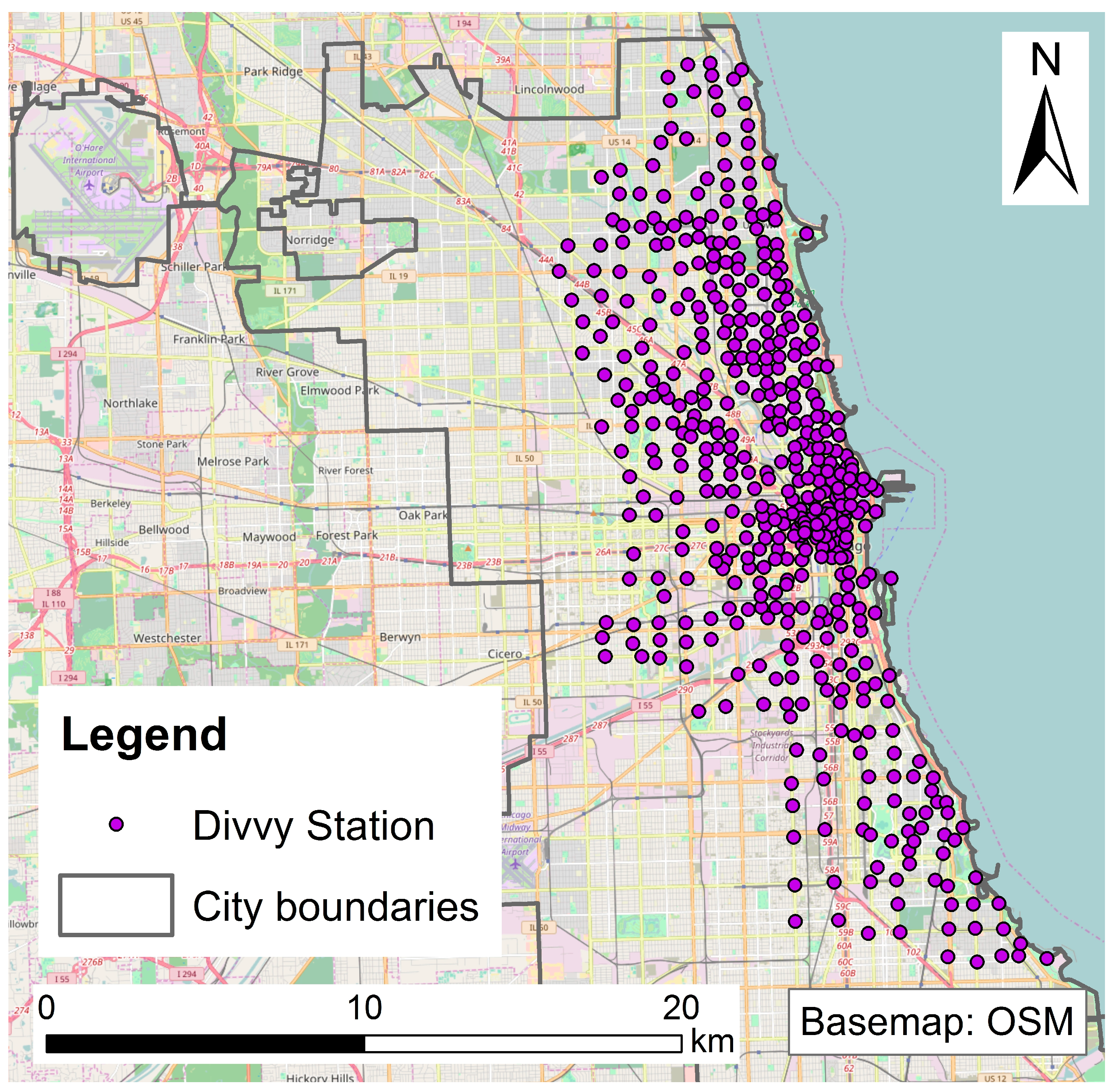
2.1.1. BSS Data

In this study, the cycling dataset was offered by Divvy (Motivate, Chicago, IL, USA), which is a BSS in Chicago. It began operating in June 2013. Yearly historical Divvy data are publicly available [42]. The 2015 data includes two files: Trips and Stations. There are 3,183,439 cycling trips and 474 docking stations in these two files, respectively. In the Trips file, each trip was anonymized and includes: bike ID, trip start day and time, trip end day and time, trip start station ID, trip end station ID, trip duration, user type. Divvy has two user types: Subscriber and Customer, representing annual members and casual users, respectively. If a trip was made by a Subscriber, gender and year-of-birth of the Subscriber is available. In the Stations file, each station includes: station ID, station name, and station location (longitude/latitude). Figure 1 maps the docking stations of Divvy in Chicago. In 2015, there were 3,183,439 cycling trips, including 2,253,556 trips made by annual members (70%) and 929,883 made by casual riders (30%). The average duration of all cycling trips was 17.1 min. Specifically, the average duration of annual members’ trips was 12.1 min; while the average duration of casual users’ trips was 29.2 min. Casual users tend to cycle for a longer duration than annual members do. On the other hand, according to an estimate based on field observations [43], the average duration of regular riders’ trips in Chicago was roughly 45 min. Compared with the average duration of regular riders’ trips, the average duration of Divvy riders’ trips is much shorter. This is mainly because only the first 30 min of the Divvy system is free and users are encouraged to use Divvy for short trips [41].

Table 1. Demographics of Divvy cycling trips of annual members in 2015.

Gender	Male			Female
Percent of trips	74.8%			25.2%
Average trip duration (min)	11.5			13.7
Age Category	Under 19	19–25	26–34	35–54	55–64	Over 64
Percent of trips	0.3%	14%	45.2%	33.7%	5.9%	0.9%
Average trip duration (min)	12.2	11.9	12.1	12.0	12.3	13.6

shows the demographics of cycling trips of Divvy’s annual members in 2015. The majority of cycling trips were made by male riders, while female riders tend to cycle for a longer duration. Users aged 26–34 years made almost half of the total cycling trips, while users aged over 64 years tended to cycle for a longer average duration.

We further removed some noisy trips by the following steps:

(1)

We first removed trips with a duration of more than 90 min (twice the average duration of regular riders’ trips in Chicago [43]), as trips longer than 90 min are not typical bicycle-sharing rides and could also be a result of misplacing the bicycle when returning it to the station [41];

(2)

We further removed trips originating or arriving at a docking station with a unique ID of ‘394’, as this docking station is missing in the Stations file and thus its geo-location is unknown.

2.1.2. Data for Environmental Factors

In this study, we took account of environmental factors, including socioeconomic factors, land use and point-of-interest (POI) factors, road infrastructure factors, public transit accessibility factors, and safety and convenience factors. Accordingly, data of residents and jobs were used to measure socioeconomic factors; land use data and data of POIs were used to measure land use and point-of-interest (POI) factors; data of road networks and bicycle lanes were used to measure road infrastructure factors; data of public transit services was used to measure public transit accessibility factors; and finally data of traffic accidents and congestion and data of violent crimes were used to measure safety and convenience factors.

Specifically, data of residents and jobs were downloaded from US Census Bureau’s Longitudinal Employer Household Dynamics (LEHD) synthetic data [44]. Data of road network, data of bicycle lanes, data of public transit services, and crime data were downloaded from Chicago’s open data portal [45]; while land use data were downloaded from Chicago Metropolitan Agency for Planning [46]. Data of POIs were downloaded from MapQuest via APIs [47]. Data of traffic accidents and congestion were downloaded from Bing Maps REST Services via APIs [48]. One-year records of geo-referenced and time-stamped traffic accidents and congestions from June 2015 to May 2016 were collected since June 2015. As Bing Maps REST Services do not support downloading historical records, we do not have records before June 2015. Instead, we used records from June 2015 to May 2016 to represent traffic accidents and congestions in this study. A three-year dataset of geo-referenced and time-stamped violent crimes from 2013 to 2015 was used to represent violent crimes. The geographical levels of population and employment were obtained from census tracts. The population and employment data in 2014 were used, as they were the most updated. Also, we used the latest land use data generated based on aerial images from 2013. The public transit data were obtained from a General Transit Feed Specification (GTFS) dataset that was downloaded from the Chicago Transit Authority (CTA) system, including stops, route patterns, and a full service schedule. The geography level and temporal level of traffic and crime data were street level and second level.

2.2. Cycling Behaviour and Investigation Model

In this study, we focused on the cycling behavior of annual members rather than casual riders because: (1) annual members tend to use BSS much more frequently than casual riders; and (2) 70% of the cycling trips were made by annual members. Accordingly, we first partitioned the cycling trips into trips made by annual members and trips made by casual riders, and then counted the cycling trips of annual members departing from or arriving at each docking station during a one-hour time slot separately. To characterize the cycling behavior of BSS riders (annual members), we measured the usage of docking stations as an origin or destination by two indices: hourly number of departures and hourly number of arrivals. A docking station’s hourly number of departures and hourly number of arrivals represent the total number of cycling trips from and to this station during a one-hour time slot (e.g., 7:00 a.m.–7:59 a.m.) on all workdays in 2015. Specifically, dependent variables are hourly number of departures and hourly number of arrivals. In this study, we investigated the impact of environmental factors on one of these two dependent variables each time. Consequently, there are 11,376 records (24 h × 474 stations) of each dependent variable.

To quantitatively examine the effects of environmental factors with different data types (numeric and categorical), a linear mixed-effects model (also called a linear mixed model) was employed in this study. Moreover, a multilevel linear mixed model was employed to explicitly recognize the dependencies associated with bicycle flows originating or arriving at the same station, as a traditional linear regression model is not appropriate for studying data with multiple repeated observations [37]. Additionally, an earlier study [37] compared a linear regression model and a linear mixed model, and its experimental results demonstrated the suitability of the mixed modeling approach employed in an analysis for examining the determinants of BSS usage.

The general form of a linear mixed model is:

$$y=X\beta +Z\gamma +\epsilon$$

(1)

where y is an N × 1 response vector of the outflows or inflows of docking stations; N is the number of observations (24 h × 474 stations); X is an N × p matrix of the p independent variables for the fixed-effects; β is an N × 1 fixed-effects vector; Z is an N × q matrix for the q random-effects; γ is a q × 1 random-effects vector; ε is an N × 1 vector of the residuals.

For simplicity, we only considered random intercepts in this study. Accordingly, we assume that: apart from the capacity and visibly environmental factors of the docking stations, some other invisibly environmental factors of the docking stations, e.g., building density, steep inclines, or the presence of tourism sites nearby, might influence cyclists’ behavior in a way that is not seen in the present data. In this study, the number of groups is equal to the number of docking stations.

2.3. Environmental Factors

In this study, we took account of population density, employment density, land use mix, accessibility to POIs (schools, shops, parks and gyms), road infrastructure, public transit accessibility, road safety and convenience, and public safety.

Table 2. Independent variables considered in this study.

Categories of Factors	Independent Variables	Type	Varying Type
Non-environmental factors	Station capacity	numeric	-
	Time of day	categorical	-
Socioeconomic factors	Residential density (/km square)	numeric	Spatially varying
	Employment density (/km square)	numeric	Spatially varying
Road infrastructure factors	Length of roads (m)	numeric	Spatially varying
	Length of bicycle lanes (m)	numeric	Spatially varying
Land use and POI factors	Land use mix	numeric	Spatially varying
	Presence of colleges and universities	categorical	Spatially varying
	Presence of schools	categorical	Spatially varying
	Presence of grocery stores	categorical	Spatially varying
	Presence of retail shops	categorical	Spatially varying
	Presence of gyms	categorical	Spatially varying
	Presence of parks	categorical	Spatially varying
Public transit service factors	Metro frequency	numeric	Spatially varying
	Hourly bus frequency	numeric	Spatiotemporally varying
Road safety and convenience factors	Number of traffic accidents	numeric	Spatiotemporally varying
	Number of traffic congestions	numeric	Spatiotemporally varying
Public safety factors	Number of on-street violent crimes	numeric	Spatiotemporally varying
	Number of off-street violent crimes	numeric	Spatiotemporally varying

lists the independent variables, including station capacity, time of the day, and environmental variables. Station capacity is the capacity of each docking station. Time of the day is classified into six categories: Very Early AM Hours (12:00 p.m.–3:59 a.m.), Early AM Hours (4:00 a.m.–5:59 a.m.), AM Peak Hours (6:00 a.m.–8:59 a.m.), Mid-Day Hours (9:00 a.m.–2:59 p.m.), PM Peak Hours (3:00 p.m.–5:59 p.m.), Early Evening Hours (6:00 p.m.–7:59 p.m.), and Late Evening Hours (8:00 p.m.–11:59 p.m.).

We characterized the environmental factors at the level of the station’s surrounding area. Here, the surrounding area of a docking station is defined as a circular buffer surrounding the docking station. An earlier study [41] suggests that a 300-m buffer around each station was found to be an appropriate walking distance, considering the distances between Divvy stations in the city of Chicago [11]. Therefore, we set a radius of 300 m to define the surrounding area for each docking station.

Based on the 300-m surrounding area, the environmental variables of docking station are defined and calculated as follows:

Residential density and employment density is the density of residents and jobs in the 300-m buffer. As a docking station’s buffer might overlap more than one census tract, we combined all overlapping parts of census tracts and the 300-m buffer. Supposing that i is a docking station, we calculated residential density and employment density of its buffer as:

$$\begin{gathered} res\_den \left(i\right)={\displaystyle \sum }_{i\in S\left(i\right)}res\_den{ }^{sub} \left(i,j\right)\times \frac{area{ }^{sub} \left(i,j\right)}{sum\_area{ }^{sub} \left(i\right) } \\ emp\_den \left(i\right)={\displaystyle \sum }_{i\in S\left(i\right)}emp\_den{ }^{sub} \left(i,j\right)\times \frac{area{ }^{sub} \left(i,j\right)}{sum\_area{ }^{sub} \left(i\right) } \\ sum\_area{ }^{sub} \left(i\right)={\displaystyle \sum }_{i\in S\left(i\right)}area{ }^{sub} \left(i,j\right) \end{gathered}$$

(2)

where $res\_de{n}^{sub} \left(i,j\right)$ and $emp\_de{n}^{sub}\left(i,j\right)$ represent the residential density and employment density of the overlapping part of census tract j and the buffer, equaling residential density and employment density of census tract j. $Area{ }^{sub} \left(i,j\right)$ represents the area of the overlapping part of census tract j and the buffer; $S\left(i\right)$ is the set of overlapping parts of census tracts and the buffer.

Length of roads equals the total length of roads within the 300-m buffer. It is used to measure the density of roads. As the buffer of each docking station is same size, the length of roads is not necessarily divided by the area of the buffer to represent the level of road density.

Length of bicycle lanes equals the total length of bicycle lanes within the 300-m buffer. It is used to measure the level of cycling facilities.

Land use mix is the mix level of land use in the 300-m buffer. We used an entropy index to describe the level of land use mix [28,49]. The higher the entropy index, the more homogeneous the distribution of land types; in other words, the higher the level of land use mix. Supposing that there are N land use types, the entropy-based land use mix is represented as:

$$LandUse\_Entropy=-{\displaystyle \sum }_{t=1}^N\frac{LUA\left(t\right)}{LUA } lo{g}_2\frac{LUA\left(t\right)}{LUA }$$

(3)

where: LUA (t) represents the area of land use type t in the 300-m buffer; LUA represents the total area of all of the land use types. In this study, N equals 7. The seven land use types are: commercial, residential, industrial, institutional, other built-in, open space, and others. The entropy-based land use mix is within the range of 0 to 1, with 0 meaning a single land use type (e.g., all residential) and 1 denoting the even distribution of all seven land use types in the 300-m buffer.

Presence of colleges and universities, presence of schools, presence of grocery stores, presence of retail shops, presence of gyms, and presence of parks represent whether there are colleges and universities, schools, grocery stores, retail shops, gyms, or parks within the 300-m buffer. As a large portion of docking stations’ 300-m buffers presented zero POI, we used a binary categorical data type instead of the original numeric data type to measure the availability of POIs. Specifically, ‘Y’ means there are colleges and universities, schools, grocery stores, retail shops, gyms, gyms, or parks within the 300-m buffer, while ‘N’ means there are none.

Metro frequency is the total number of metro routes passing all metro stations within the 300-m buffer. As the hourly frequency of each metro route is almost identical and the service times of each metro station is close to 24 h, we only calculated the number of routes to measure metro accessibility at each metro station.

Hourly bus frequency is the hourly number of bus trips passing all bus stops within the 300-m buffer on workdays (Monday to Friday). This was used to measure bus accessibility. Supposing that i is a docking station, its hourly bus frequency is calculated as:

$$Hourly\_bus\_frequency{ }_{Workday}\left(i,t\right)={\displaystyle \sum }_{j\in S\left(i\right)} ave\_num\_bus\_tri{p}_{Workday}^{Stop} \left(j,t\right)$$

(4)

where $ave\_num\_bus\_ trip{ }_{Hour}^{Stop} \left(j,t\right)$ is the average number of bus trips passing through the bus stop j during a one-hour time slot t on workdays; $S\left(i\right)$ is the set of bus stops that are situated within the 300-m buffer of i.

Number of traffic accidents and number of traffic congestions are the hourly number of traffic accidents and congestions within the 300-m buffer on workdays (Monday to Friday), respectively.

Number of on-street violent crimes and number of off-street violent crimes are the hourly number of on-street violent crimes and off-street violent crimes within the 300-m buffer on workdays, respectively.

3. Results and Discussion

In this study, 11,376 records (24 h × 474 stations) of independent variables (see Table 2) were input into a linear mixed model for annual members’ usage of BSS.

Table 3. Estimation results for the linear mixed-effects model of annual members’ usage of BSS.

Dependent Variables	Number of Departures			Number of Arrivals
	Coefficient	SE	p-Value	Coefficient	SE	p-Value
Intercept	−175.8405	53.0865	0.0009	−166.7397	54.61012	0.0023
Station capacity	12.0613	1.5291	0.0000	10.6922	1.57263	0.0000
Time of the day
Very Early AM Hours	−143.7644	11.5381	0.0000	−71.3877	12.15045	0.0000
Early AM Hours	−173.9006	12.8865	0.0000	−137.9380	14.2535	0.0000
Mid-Day Hours	−124.5655	8.9725	0.0000	−80.4140	9.67545	0.0000
PM Peak Hours	42.5995	10.3971	0.0000	64.0528	11.19967	0.0000
Early Evening Hours	11.6596	11.4634	0.3091 *	83.1189	12.34153	0.0000
Late Evening Hours	−119.6928	10.2082	0.0000	−53.0330	10.97764	0.0000
Residential density (/km2)	0.0186	0.0032	0.0000	0.0182	0.00332	0.0000
Employment density (/km2)	0.0009	0.0003	0.0007	0.0007	0.00026	0.0103
Length of roads (m)	0.0073	0.0067	0.2768 *	0.0049	0.00689	0.4777 *
Length of bicycle lanes (m)	0.0601	0.0138	0.0000	0.0575	0.01423	0.0001
Land use mix	−21.8775	22.5117	0.3316 *	−28.0693	23.15241	0.2260 *
Presence of colleges and universities	−10.0147	48.2621	0.8357 *	−37.0241	49.62023	0.4560 *
Presence of schools	−18.9770	23.4374	0.4185 *	−8.5928	24.10353	0.7216 *
Presence of grocery stores	7.1587	20.0450	0.7212 *	13.9893	20.60905	0.4976 *
Presence of retail shops	0.2341	24.4684	0.9924 *	−6.7945	25.16695	0.7873 *
Presence of gyms	17.4116	23.8579	0.4659 *	15.2305	24.53158	0.5350 *
Presence of parks	21.3966	22.8465	0.3495 *	18.7704	23.52777	0.4254 *
Metro frequency	−100.9208	9.8811	0.0000	−101.3879	10.19235	0.0000
Hourly bus frequency	1.5963	0.0481	0.0000	1.9287	0.05128	0.0000
Number of traffic accidents	−0.1345	0.0959	0.1608 *	−0.0147	0.10291	0.8865 *
Number of traffic congestions	0.1578	0.2536	0.5338 *	0.1224	0.27341	0.6543 *
Number of on-street violent crimes	1.4532	1.5760	0.3565 *	−11.0763	1.68906	0.0000
Number of off-street violent crimes	−1.3761	1.0424	0.1868 *	−4.4316	1.11484	0.0001
AIC	148,544.2			150,541.3
BIC	148,740.4			150,737.5
Restricted log-likelihood	−74,245.12			−75,243.65

Note: * means it is not statistically significant at a 0.05 level.

lists the estimation results for the linear mixed-effects model of annual members’ usage of BSS. The number of observations is 11,376, which is equal to the number of records, and the number of groups is 474, which is equal to the number of dock stations. In Table 3, the coefficient is the coefficient estimated for each independent variable in the fixed effects; the SE is the standard error for each independent variable; and the p-value indicates the statistical significance for each independent variable. In this study, a p-value below 0.05 means the corresponding independent variable is statistically significantly associated with the dependent variable at a 0.05 level. Moreover, a positive coefficient means the corresponding independent variable is positively associated with the dependent variable, while a negative coefficient means the corresponding independent variable is negatively associated with the dependent variable. We demonstrated and discussed the environmental effects on annual members’ usage of BSS.

3.1. Environmental Effect on Annual Members’ Usage of BSS

We first examined the effects of independent variables on annual members’ usage of BSS. Unsurprisingly, station capacity is positively and significantly associated with both number of departures and number of arrivals. Regarding time of the day, annual members are more likely to use BSS during PM Peak Hours (3:00 p.m.–5:59 p.m.) and Early Evening Hours (6:00 p.m.–7:59 p.m.), while annual members are less likely to use BSS during the other times of the day. This coincides with a finding in an earlier study: the BSS in Montreal is more predominantly used during the PM period (3:00 p.m.–7 p.m.) relative to other times of the day [37]. Of the socioeconomic factors, both residential density and employment density are positively and significantly associated with both number of departures and number of arrivals. Of the infrastructure factors, length of roads is not significantly associated with number of departures or number of arrivals, while length of bicycle lanes is positively and significantly associated with both number of departures and number of arrivals. None of the land use and POI factors (land use mix, presence of colleges and universities, presence of schools, presence of grocery stores, presence of retail shops, presence of gyms, and presence of parks) are significantly associated with number of departures or number of arrivals. Interestingly, hourly bus frequency is positively and significantly associated with both number of departures and number of arrivals, while metro frequency is negatively and significantly associated with both number of departures and number of arrivals. More interestingly, two road safety and convenience factors (number of traffic accidents and number of traffic congestions) are not significantly associated with number of departures or number of arrivals, while two public safety factors (number of on-street violent crimes and number of off-street violent crimes) are negatively and significantly associated with number of arrivals but are not significantly associated with number of departures.

3.2. Discussion and Implications for Policies

We further discussed the environmental effects on the usage of BSS, and then tried to offer implications for policies. First of all, the socioeconomic factors, both residential density and employment density tend to increase the usage of BSS as they tend to be positively associated with the demand for BSS. Second, of the infrastructure factors, length of roads does not influence the usage of BSS, while length of bicycle lanes tends to increase the usage of BSS. This suggests that an increase in bicycle lanes separated from motor traffic is likely to increase the usage of BSS. Third, the usage of BSS is influenced by none of the land use or POI factors, i.e., land use mix and presence of colleges and universities, schools, grocery stores, retail shops, gyms, and parks. Fourth, of the public transit service factors, hourly bus frequency influences the usage of BSS differently than metro frequency. As mentioned above, the average duration of BSS riders’ trips is much shorter than that of regular riders’ trips. Most of the BSS riders’ trips tend to be only part of the BSS riders’ complete origin-destination trips, considering the short average duration of BSS riders’ trips and the lack of docking stations near some workplaces or homes. Therefore, BSS riders might need to use public transport or car to complete their origin-destination trips. It is inferable that public transit accessibility tends to be positively associated with the usage of BSS, as some earlier studies uncovered. Surprisingly, this study revealed that metro accessibility influences the usage of BSS in a different way. Specifically, hourly bus frequency is positively associated with the usage of BSS, while metro frequency is negatively associated with the usage of BSS. This indicates that BSS riders are likely to transfer between BSS and bus but are unlikely to transfer between BSS and metro. Fifth, neither number of traffic accidents nor number of traffic congestions influences the usage of BSS. This contradicts our expectation that a large number of traffic accidents or traffic congestions would reduce the usage of BSS. Sixth, both number of on-street violent crimes and number of off-street violent crimes tend to decrease the usage of BSS. This coincides with our expectation that a large number of on-street violent crimes tend to reduce the usage of BSS, and a large number of off-street violent crimes might increase the usage of BSS as well.

Finally, we linked the environmental effects with policies to offer some implications for increasing the usage of BSS and for the site selection of new docking stations. Specifically, this study suggests that: (1) investment in cycling facilities tends to increase the usage of BSS; (2) reducing violent crimes is likely to encourage people to use BSS; and (3) residential density, employment density, public transit service, levels of cycling facilities, and the rate of violent crimes should be considered in the site selection of new docking stations.

4. Conclusions

This study has investigated the impacts of environmental characteristics on the usage of BSS, and tried to offer suggestions for policies aiming to increase the usage of BSS or to choose the sites of new docking stations. Empirical results demonstrated that the density of bicycle lanes, public transit accessibility, and public safety influence the usage of BSS. We obtained answers to the following research questions: (1) neither traffic accidents nor traffic congestion influences the usage of BSS; (2) both on-street violent crimes and off-street violent crimes tend to decrease the usage of BSS; (3) bus accessibility is positively associated with the usage of BSS, while metro accessibility is negatively associated with the usage of BSS. Empirical results also suggested the policy implications that improving bicycle facilities and reducing the rate of violent crimes tend to increase the usage of BSS. Moreover, some environmental factors could be considered in selecting a site for a new docking station.

4.1. Limitations

There are some limitations to this study. First, as how often each member uses BSS is unknown, we were not able to access the annual or monthly average frequency of BSS usage at the individual level. Ideally, individual-level frequency of BSS usage would be known, and we thus would be able to investigate the environmental effects on the cycling behavior of BSS riders at an individual level. Second, the cycling purpose of BSS usage is unknown. Ideally, the cycling purpose of members’ BSS usage would be known, and we thus could examine how BSSs increase commuting and recreational cycling, respectively.

4.2. Future Works

In future research, some aspects should be considered for further study. First, route choice modelling could be used to infer the explicit cycling paths based on road networks and cyclists’ preferences [22]. Second, to understand how BSS usage may increase with the number of docking stations and operating years, we could explore the monthly variations of BSS usage from 2013 to 2017, as Divvy offers data for several different years. Third, comparing the cycling behavior of BSS riders and private bicycle riders is also interesting. Traffic count data [50] or crowdsourced data from online social networking websites for sports, such as Strava [51,52], could be used as cycling data for private bicycle riders.

References

- Cavill, N.; Davis, A. Cycling and Health: What’s the Evidence? Cycling England: London, UK, 2007. [Google Scholar]
- Forsyth, A.; Krizek, K.J.; Agrawal, A.W.; Stonebraker, E. Reliability testing of the Pedestrian and Bicycling Survey (PABS) method. J. Phys. Act. Health 2012, 9, 677–688. [Google Scholar] [CrossRef] [PubMed]
- Oja, P.; Vuori, I.; Paronen, O. Daily walking and cycling to work: Their utility as health-enhancing physical activity. Patient Educ. Couns. 1998, 33 (Suppl. 1), S87–S94. [Google Scholar] [CrossRef]
- Oja, P.; Titze, S.; Bauman, A.; de Geus, B.; Krenn, P.; Reger-Nash, B.; Kohlberger, T. Health benefits of cycling: A systematic review. Scand. J. Med. Sci. Sports 2011, 21, 496–509. [Google Scholar] [CrossRef] [PubMed]
- Pucher, J.; Buehler, R.; Bassett, D.R.; Dannenberg, A.L. Walking and cycling to health: A comparative analysis of city, state, and international data. Am. J. Public Health 2010, 100, 1986–1992. [Google Scholar] [CrossRef] [PubMed]
- Taddei, C.; Gnesotto, R.; Forni, S.; Bonaccorsi, G.; Vannucci, A.; Garofalo, G. Cycling promotion and non-communicable disease prevention: Health impact assessment and economic evaluation of cycling to work or school in Florence. PLoS ONE 2015, 10, e0125491. [Google Scholar] [CrossRef] [PubMed]
- Wen, L.M.; Rissel, C. Inverse associations between cycling to work, public transport, and overweight and obesity: Findings from a population based study in Australia. Prev. Med. 2008, 46, 29–32. [Google Scholar] [PubMed]
- Maizlish, N.; Woodcock, J.; Co, S.; Ostro, B.; Fanai, A.; Fairley, D. Health co-benefits and transportation-related reductions in greenhouse gas emissions in the San Francisco Bay area. Am. J. Public Health 2013, 103, 703–709. [Google Scholar] [CrossRef] [PubMed]
- Woodcock, J.; Givoni, M.; Morgan, A. Health impact modelling of active travel visions for England and Wales using an Integrated Transport and Health Impact Modelling tool (ITHIM). PLoS ONE 2013, 8, e51462. [Google Scholar] [CrossRef] [PubMed]
- De Hartog, J.; Boogaard, H.; Nijland, H.; Hoek, G. Do the health benefits of cycling outweigh the risks? Environ. Health Perspect. 2010, 118, 1109–1116. [Google Scholar] [CrossRef] [PubMed]
- Shaheen, S.; Martin, E.; Cohen, A. Public bikesharing and modal shift behavior: A comparative study of early bikesharing systems in North America. Int. J. Transp. 2013, 1, 35–53. [Google Scholar] [CrossRef]
- Forsyth, A.; Krizek, K. Urban design: Is there a distinctive view from the bicycle? J. Urban Des. 2011, 16, 531–549. [Google Scholar] [CrossRef]
- Furness, Z. One Less Car: Bicycling and the Politics of Automobility; Temple University Press: Philadelphia, PA, USA, 2010. [Google Scholar]
- Gatersleben, B.; Uzzell, D. Affective appraisals of the daily commute: Comparing perceptions of drivers, cyclists, walkers, and users of public transport. Environ. Behav. 2007, 39, 416–431. [Google Scholar] [CrossRef]
- Heinen, E.; van Wee, B.; Maat, K. Commuting by bicycle: An overview of the literature. Transp. Rev. 2010, 30, 59–96. [Google Scholar] [CrossRef]
- Lawson, A.R.; Pakrashi, V.; Ghosh, B.; Szeto, W.Y. Perception of safety of cyclists in Dublin city. Accid. Anal. Prev. 2013, 50, 499–511. [Google Scholar] [CrossRef] [PubMed]
- Møller, M.; Hels, T. Cyclists’ perception of risk in roundabouts. Accid. Anal. Prev. 2008, 40, 1055–1062. [Google Scholar] [CrossRef] [PubMed]
- Perkins, C.; Thomson, A.Z. Mapping for health: Cycling and walking maps of the city. North West Geogr. 2005, 5, 16–23. [Google Scholar]
- Pucher, J.; Dill, J.; Handy, S. Infrastructure, programs, and policies to increase bicycling: An international review. Prev. Med. 2010, 50, S106–S125. [Google Scholar] [CrossRef] [PubMed]
- Reddy, S.; Shilton, K.; Denisov, G.; Cenizal, C.; Estrin, D.; Srivastava, M. Biketastic: Sensing and mapping for better biking. In Proceedings of the SIGCHI Conference on Human Factors in Computing Systems, Atlanta, GA, USA, 10–15 April 2010; pp. 1817–1820. [Google Scholar]
- Pánek, J.; Benediktsson, K. Emotional mapping and its participatory potential: Opinions about cycling conditions in Reykjavík, Iceland. Cities 2017, 61, 65–73. [Google Scholar] [CrossRef]
- Woodcock, J.; Tainio, M.; Cheshire, J.; O’Brien, O. Health effects of the London bicycle sharing system: Health impact modelling study. BMJ 2014, 348, g425. [Google Scholar] [CrossRef] [PubMed]
- Rojas-Rueda, D.; de Nazelle, A.; Tainio, M.; Nieuwenhuijsen, M.J. The health risks and benefits of cycling in urban environments compared with car use: Health impact assessment study. BMJ 2011, 343, 4521. [Google Scholar] [CrossRef] [PubMed]
- Fishman, E.; Washington, S.; Haworth, N. Bike share’s impact on car use: Evidence from the United States, Great Britain, and Australia. Transp. Res. Part D Transp. Environ. 2014, 31, 13–20. [Google Scholar] [CrossRef]
- Garrard, J.; Rose, G.; Lo, S.K. Promoting transportation cycling for women: The role of bicycle infrastructure. Prev. Med. 2008, 46, 55–59. [Google Scholar] [CrossRef] [PubMed]
- Carver, A.; Salmon, J.; Campbell, K.; Baur, L.; Garnett, S.; Crawford, D. How do perceptions of local neighborhood relate to adolescents’ walking and cycling? Am. J. Health Promot. 2005, 20, 139–147. [Google Scholar] [CrossRef] [PubMed]
- Hunt, J.D.; Abraham, J.E. Influences on bicycle use. Transportation 2007, 34, 453–470. [Google Scholar] [CrossRef]
- De Vries, S.I.; Hopman-Rock, M.; Bakker, I.; Hirasing, R.A.; van Mechelen, W. Built environmental correlates of walking and cycling in Dutch urban children: Results from the SPACE study. Int. J. Environ. Res. Public Health 2010, 7, 2309–2324. [Google Scholar] [CrossRef] [PubMed]
- Fraser, S.; Lock, K. Cycling for transport and public health: A systematic review of the effect of the environment on cycling. Eur. J. Public Health 2010, 21, 738–743. [Google Scholar] [CrossRef] [PubMed]
- Mäki-Opas, T.E.; Borodulin, K.; Valkeinen, H.; Stenholm, S.; Kunst, A.E.; Abel, T.; Härkänen, T.; Kopperoinen, L.; Itkonen, P.; Prättälä, R.; et al. The contribution of travel-related urban zones, cycling and pedestrian networks and green space to commuting physical activity among adults—A cross-sectional population-based study using geographical information systems. BMC Public Health 2016, 16, 760. [Google Scholar] [CrossRef] [PubMed]
- Fishman, E. Bikeshare: A review of recent literature. Transp. Rev. 2016, 36, 92–113. [Google Scholar] [CrossRef]
- Garcia-Palomares, J.C.; Gutierrez, J.; Latorre, M. Optimizing the location of stations in bike-sharing programs: A GIS approach. Appl. Geogr. 2012, 35, 235–246. [Google Scholar] [CrossRef]
- Shaheen, S.; Zhang, H.; Martin, E.; Guzman, S. Hangzhou public bicycle: Understanding early adoption and behavioral response to bike sharing in Hangzhou, China. Transp. Res. Rec. 2011, 2247, 5. [Google Scholar] [CrossRef]
- Fuller, D.; Gauvin, L.; Kestens, Y.; Daniel, M.; Fournier, M.; Morency, P.; Drouin, L. Use of a new public bicycle share program in Montreal, Canada. Am. J. Prev. Med. 2011, 41, 80–83. [Google Scholar] [CrossRef] [PubMed]
- Molina-Garcia, J.; Castillo, I.; Queralt, A.; Sallis, J.F. Bicycling to university: Evaluation of a bicycle-sharing program in Spain. Health Promot. Int. 2015, 30, 350–358. [Google Scholar] [CrossRef] [PubMed]
- Rixey, R. Station-Level Forecasting of Bikesharing Ridership: Station Network Effects in Three U.S. Systems. Transp. Res. Rec. 2013, 2387, 6. [Google Scholar] [CrossRef]
- Faghih-Imani, A.; Eluru, N.; El-Geneidy, A.M.; Rabbat, M.; Haq, U. How land-use and urban form impact bicycle flows: Evidence from the bicycle-sharing system (BIXI) in Montreal. J. Transp. Geogr. 2014, 41, 306–314. [Google Scholar] [CrossRef]
- El-Assi, W.; Salah Mahmoud, M.; Nurul Habib, K. Effects of built environment and weather on bike sharing demand: A station level analysis of commercial bike sharing in Toronto. Transportation 2017, 44, 589–613. [Google Scholar] [CrossRef]
- Buck, D.; Buehler, R. Bike lanes and other determinants of capital bike share trips. In Proceedings of the 91st Annual Meeting of the Transportation Research Board, Washington, DC, USA, 22–26 January 2012. [Google Scholar]
- Fishman, E.; Washington, S.; Haworth, N.; Watson, A. Factors influencing bike share membership: An analysis of Melbourne and Brisbane. Transp. Res. Part A Policy Pract. 2015, 71, 17–30. [Google Scholar] [CrossRef]
- Faghih-Imani, A.; Eluru, N. Analysing bicycle-sharing system user destination choice preferences: Chicago’s Divvy system. J. Transp. Geogr. 2015, 44, 53–64. [Google Scholar] [CrossRef]
- Divvy. Divvy Data. Available online: https://www.divvybikes.com/system-data (accessed on 1 January 2016).
- Caldwell, J.; O’Neil, R.; Schwieterman, J.P.; Yanocha, D. Policies for Pedaling: Managing the Tradeoff between Speed & Safety for Biking in Chicago; Chaddick Institute for Metropolitan Development, DePaul University: Chicago, IL, USA, 2016; Available online: https://las.depaul.edu (accessed on 1 December 2016).
- US Census Bureau. Longitudinal Employer-Household Dynamics. Available online: https://lehd.ces.census.gov (accessed on 1 August 2015).
- City of Chicago’s Open Data Portal. Available online: https://data.cityofchicago.org (accessed on 1 January 2016).
- Chicago Metropolitan Agency for Planning. CMAP Data. Available online: http://www.cmap.illinois.gov (accessed on 14 January 2016).
- MapQuest. Available online: https://developer.mapquest.com/ (accessed on 1 December 2011).
- Bing Maps REST Services. Available online: https://msdn.microsoft.com/en-us/library/hh441725.aspx (accessed on 1 April 2008).
- Larsen, K.; Gilliland, J.; Hess, P.; Tucker, P.; Irwin, J.; He, M. The influence of the physical environment and sociodemographic characteristics on children’s mode of travel to and from school. Am. J. Public Health 2009, 99, 520–526. [Google Scholar] [CrossRef] [PubMed]
- El Esawey, M. Estimation of annual average daily bicycle traffic with adjustment factors. Transp. Res. Rec. 2014, 2443, 106–114. [Google Scholar] [CrossRef]
- Griffin, G.P.; Jiao, J. Where does bicycling for health happen? Analysing volunteered geographic information through place and plexus. J. Transp. Health 2015, 2, 238–247. [Google Scholar] [CrossRef]
- Sun, Y.; Mobasheri, A. Utilizing Crowdsourced Data for Studies of Cycling and Air Pollution Exposure: A Case Study Using Strava Data. Int. J. Environ. Res. Public Health 2017, 14, 274. [Google Scholar] [CrossRef] [PubMed]