Article

Comparative Analysis of Decoupling Control Methodologies and H Multivariable Robust Control for Variable-Speed, Variable-Pitch Wind Turbines: Application to a Lab-Scale Wind Turbine

1
Department of Computer Science and Numerical Analysis, Universidad de Córdoba, Campus de Rabanales, 14071 Cordoba, Spain
2
Department of Computer Science and Automatic Control, Universidad Nacional de Educación a Distancia, Juan del Rosal 16, 28040 Madrid, Spain
*
Author to whom correspondence should be addressed.
Sustainability 2017, 9(5), 713; https://doi.org/10.3390/su9050713
Submission received: 21 February 2017 / Revised: 4 April 2017 / Accepted: 27 April 2017 / Published: 29 April 2017
(This article belongs to the Special Issue The Impact and Innovation of Wind Turbine Technologies)

Abstract

:
This work is focused on the improvement of variable-speed variable-pitch wind turbine performance by means of its control structure. This kind of systems can be considered as multivariable nonlinear processes subjected to undesired interactions between variables and presenting different dynamics at different operational zones. This interaction level and the dynamics uncertainties complicate the control system design. The aim of this work is developing multivariable controllers that cope with such problems. The study shows the applicability of different decoupling methodologies and provides a comparison with a H controller, which is an appropriate strategy to cope with uncertainties. The methodologies have been tested in simulation and verified experimentally in a lab-scale wind turbine. It is demonstrated that the wind turbine presents more interaction at the transition zone. Then, this operational point is used as the nominal one for the controller designs. At this point, decoupling controllers obtain perfect decoupling while the H control presents important interaction in the generated power loop. On the other hand, they are slightly surpassed by the robust design at other points, where perfect decoupling is not achieved. However, decoupling controllers are easier to design and implement, and specifically dynamic simplified decoupling achieve the best global response. Then, it is concluded that the proposed methodologies can be considered for implantation in industrial wind turbines to improve their performance.

1. Introduction

Wind power has maintained an increasing interest since 1990, especially in the European Union, the United States and China where the average growth rate in recent years is about 20%, 25% and 50%, respectively. Global warming and energy shortage concerns encourage us to improve continuously these systems that generate carbon-emission-free electricity. System control and optimization are research areas where such enhancement can be achieved. The study presented in this work is in line with this idea in the goal to improve the wind turbine performance by means of its control structure, concretely by means of decoupling control and H control. The initial simulation developments were introduced in [1] and here they are extended and applied to an experimental lab-scale system. The proposed controllers are designed for variable-speed, variable-pitch (VS-VP) wind turbines. The aim is to track electrical power and rotor speed references while coping with process uncertainties and dynamic interactions as main difficulties.
Wind turbines can work in several operational modes or regions depending on the wind speed: cut-in (I); partial load (II); transition (III); full load (IV); and cut-out (V), as it is illustrated in Figure 1 where the ideal power curve of wind turbine is shown. When the wind speed is below its nominal value (region II), the control objective is to maximize the power captured from the wind. Over the nominal wind speed (region IV), the control goal is to maintain the power output at the rated power [2].
Although two control inputs (pitch angle and generator torque) are usually available, typical power control schemes use blade pitch angle as the only control input to keep the torque constant at its nominal value [3,4]. This monovariable strategy cannot meet simultaneously the electrical power and rotor speed regulations. Sometimes the generator torque is controlled in region II depending on the wind speed. Then, different controllers are toggled depending on the operation mode of the wind turbine. However, wind turbines are multivariable complex systems that show strong interaction between variables. This fact can cause difficulties in feedback controller design. When the wind turbines are addressed as multivariable processes, the problem of interaction is rarely well treated. Traditionally, these kinds of problems have been solved using single-loop proportional-integral-derivative (PID) controllers [5]. This approach is appropriate when the interaction is moderate. However, the system performance can deteriorate when the interaction level between variables is important. These interactions particularly occur at the transition mode (region III) between partial load mode (region II) and full load mode (region IV).
In addition, the wind turbine dynamic response is different in each operational mode. This response variability means that the system implies a multi-model process. Due to the complexity of this multi-model process from the control point of view, it could be appropriate to implement a controller that can withstand these uncertainties. Therefore, more advanced multivariable control strategies are necessary for wind turbines. This has been a field of interest as it is reported by several works developing different multivariable control methodologies: from traditional decentralized PID controllers [6] to more advanced techniques, such as fuzzy logic controllers [7,8], neural network-based controls [9,10], model predictive controls [11,12], robust H controls [13], optimal linear quadratic Gaussian (LQG) controls [14,15], linear parameter varying (LPV) controls [16,17], and nonlinear controls [18,19].
In line with these techniques, this work addresses the wind turbine control from two different points of view regarding multivariable control: decoupling and robust control. The general control scheme is depicted in Figure 2. The wind turbine is here considered as a two-input two-output system where the rotational speed ωr and the generated electric power Pg are the two controlled variables, and the blade pitch angle β and the duty cycle α are the two manipulated variables. As it is explained in next section, the duty cycle α is a signal related to the electrical torque in the experimental lab-scale wind turbine. The wind speed v is assumed to be a disturbance input for the process.
As first approach, several decoupling controls are designed to reduce the interaction problem and to achieve a good performance in all operational regions. The proposed centralized approach combines a decoupling block with a diagonal decentralized control [20]. There are distinct decoupling networks with different advantages and disadvantages. In this work, three decoupling networks are compared. As second approach, a multivariable robust H controller based on the mixed sensitivity problem is also designed and compared with the previous ones. This method is focused on coping with process uncertainties [21].
These methodologies have been simulated and tested experimentally using a linear model of a lab-scale VS-VP wind turbine. Results demonstrate that both methods obtain good system responses in different operation regions. Although robust H control yields somewhat better performance at different operation regions, it is more difficult to design and implement. From a practical view, the proposed decoupling networks are easier to implement and modify and they obtain an acceptable response over the operation range of the wind turbine. The paper is structured as follows: Section 2 presents a general description of the lab-scale wind turbine and approximated linear models that are obtained from an identification process. Section 3 explains the control methodologies and describes specifically the proposed designs for the wind turbine system under study. In Section 4, simulation and experimental results are presented and discussed. Finally, conclusions are summarized in Section 5.

2. Lab-Scale Wind Turbine and Model Description

The experimental system is a lab-scale VS-VP wind turbine that includes a rotor with two blades and direct coupling without a gearbox to a permanent magnet DC electric generator (see Figure 3). This small wind turbine emulates the dynamic response of a large-scale one with some simplifications in the electrical subsystem. The rotor and generator are placed in a small wind tunnel that has four platens to channel the wind flow towards the blades. The profile of wind speed is generated by means of a controlled fan. The wind flow crosses a grille to turn the turbulent flow into laminar. The technical parameters of the system are summarized in Table 1. The process is controlled by a computer where the controllers are implemented using the Real-Time Windows Target toolbox of Matlab/Simulink for additional educational purposes [22].
The general structure of a wind turbine is composed of a mechanical subsystem and an electrical subsystem. The mechanical subsystem consists of a turbine rotor, including the aerodynamic components, a gearbox (if any) and the low-speed and high-speed axes. The electrical subsystem is composed of a generator unit, which includes the electric generator and the static converter that is connected to a load or grid [23,24]. Next subsections summarize the physical description of these two subsystems for the lab-scale wind turbine under study as well as the mathematical relationships between its main variables from a control point of view.

2.1. Mechanical Subsystem

Assuming a rigid speed shaft and a direct coupling between the electric generator and the rotor, the dynamic of this subsystem can be described by a one-mass model [19], such as:
J t d ω r d t = τ a τ e m ,
where ωr is the rotor speed, τem is the electromagnetic torque of the generator and τa is the aerodynamic torque. Jt is the total inertia moment. The aerodynamic torque is provided by the wind forces and it depends on the turbine aerodynamic features [25]. The torque τa is given by the nonlinear expression:
τ a = 1 2 ρ π R 3 C p ( λ , β ) λ v 2 ,
where R is the radius of the rotor, v is the wind speed, and λ is the tip-speed ratio (TIP), which is defined as the ratio between the linear blade tip speed and the wind speed, as follows:
λ = ω r R v .
The power coefficient Cp(λ,β) has also effects on the aerodynamic torque and depends on the tip-speed ratio and the blade pitch angle β. It is the most important parameter for the system control design of wind turbines, especially in the power regulation case [26]. Given a wind speed, the wind turbine can be forced to work at different power coefficient conditions by means of the blade pitch angle, which acts as a manipulated variable of the system. Operation conditions with higher power coefficient imply higher performance. This coefficient Cp(λ,β) considerably contributes to the non-linear character of the process. It is difficult to obtain in practice and it is different for every wind turbine. In this work, the power coefficient is modeled from experimental data. Firstly, for a given constant blade pitch angle (β), the curve relating the power coefficient with the tip-speed ratio is obtained by a second order polynomial fitting. The same procedure is performed for 26 different pitch values obtaining different parameters. Figure 4 shows the polynomial fittings for the cases of β = 1°, β = 5°, β = 10° and β = 15°, as examples. Then, by extrapolation techniques, a three-dimensional representation of the power coefficient is obtained as a function of the tip-speed ratio and pitch angle. Figure 5 shows the corresponding surface for the experimental power coefficient of the lab-scale wind turbine. In Figure 4 and Figure 5, it can be appreciated that the optimum point is achieved at a tip-speed ratio of 6.8 and a pitch angle of 1°.

2.2. Electrical Subsystem

The lab-scale wind turbine uses a permanent-magnet DC electric generator with a constant field flux. Therefore, the electromagnetic torque τem can be modified by controlling the armature current ig according to Equation (4). Thus, a change in the generated torque conditions produces a change in the power conditions (Equation (5)). The constants η and kt symbolize the efficiency and the torque constant of the generator, respectively.
τ e m = k t i g
P g = η τ e m ω r
The armature current flows across the load. The generated torque and the electric power can be modified by changing this current. For this modification, it is necessary a variable load to be available at the generator output [27]. In the lab-scale plant, the variable load is emulated by means of a variable resistance which is implemented using a pulse-width-modulation (PWM) circuit. Using a 2 kHz PWM signal of a generic microcontroller, the resistor is connected and disconnected obtaining an apparent resistance that can be modified as a function of the duty cycle α between the nominal resistance (at 100% of duty cycle) and an open circuit, or infinite resistance, (at 0% of duty cycle). Hence, changing the duty cycle α of this PWM circuit allows modifying the electromagnetic torque. For instance, the increase of the duty cycle reduces the resistance, causing a larger current ig to flow through the generator, which increases τem.

2.3. Linear Models

In this work, the proposed control methodologies are based on linear systems. Therefore, it is necessary to obtain approximated linear models of the lab-scale wind turbine in order to perform the designs. The linear models are obtained by identification and they are defined in accordance with Equation (6), where G(s) is the process transfer matrix, and GD(s) is the disturbance matrix associated with the wind speed. The multivariable model is a two-input two-output (TITO) system. The process inputs are the duty cycle α, in the range 0–100%, and the blade pitch angle β, which ranges from 0° to 25°. The process outputs are the rotational speed ωr and the generated electric power Pg. The wind speed v is considered as process disturbance input.
( ω r P g ) =   G ( s ) ( β α ) + G D ( s ) v
Several models were identified at different operational modes depending on the wind speed. The resultant transfer matrices are listed in Table 2. There are two models at the partial load region (with wind speeds of 6 and 7 m/s), one at the transition load (8 m/s), and two at the full load region (wind speeds of 9 and 10 m/s). The identification process was performed by means of open loop step tests.
The resultant model obtained at the transition zone with a wind speed of 8 m/s was considered as the nominal model for the controller design procedures because the wind turbine experiences more interaction in this zone, as it is shown in the next subsection. Figure 6 compares the open loop step responses of the experimental data and the identified model at this point. Experimental data for obtaining g11(s) and g21(s) were generated using a ±8° step in the blade pitch angle, and those for g12(s) and g22(s) were produced applying a ±10% step in the duty cycle. The transfer functions gD1(s) and gD2(s) of GD(s) were obtained using a ±1 m/s step in the wind speed profile. Similar results and good fittings were achieved for the other tests. The variable shown in Figure 6 are relative to the initial conditions of the experiments.

2.4. Interaction Analysis

Multivariable control becomes more difficult than the monovariable counterpart due to the interaction between variables. To select the appropriate control strategy, it is important to determine this interaction level. The relative gain array (RGA) is one of the most common tools for this purpose [28]. It is based on the steady-state information of the process. Values of the element λ11 of the RGA far from the unity indicate important interaction effects. Table 3 shows the element λ11 of the RGA for the models collected in Table 2. The analysis shows that the lab-scale wind turbine has the highest interaction level at the transition operating mode (with wind speed of 8 m/s), as mentioned previously. Therefore, this study proposes designing and tuning the multivariable controllers for the corresponding model at this point, which is the most problematic. Subsequently, it is necessary to determine whether the performance is appropriate near the other operation points.

3. Controllers Design

In this section, the proposed multivariable control methodologies for the lab-scale wind turbine are described. A robust control methodology based on the H mixed sensitivity problem and three decoupling methodologies are developed. Concretely, the decoupling techniques are dynamic simplified decoupling, static simplified decoupling and inverted decoupling.

3.1. Decoupling Control

There are two approaches for multivariable control: a pure centralized strategy or a decoupling network combined with a diagonal decentralized controller [21,29]. This work considers the second approach where the control system is designed by combining a diagonal controller C(s) with a block compensator D(s) in such a way that the controller sees the apparent process Q(s) = G(s)∙D(s) as a set of completely independent processes, that is, Q(s) is diagonal or diagonally dominant. The essence of decoupling is the imposition of a calculation net that cancels the process interactions, allowing independent control of the loops [20,30]. Some decoupling schemes are static [31] and other are dynamic [29,
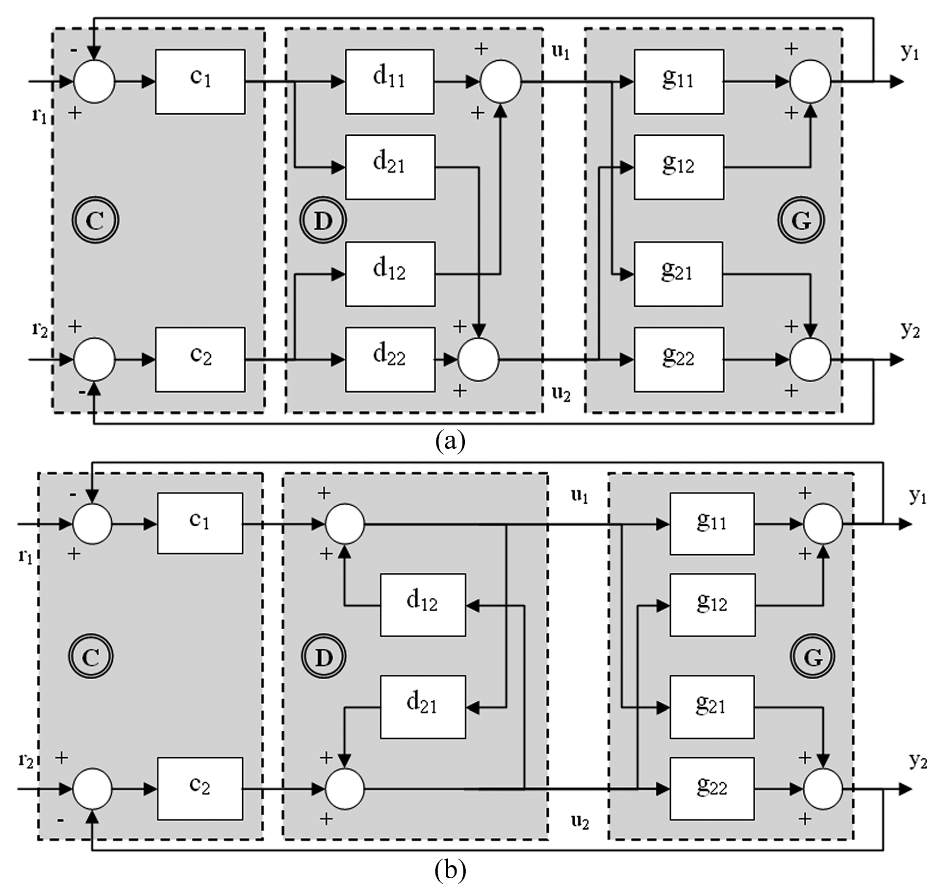
32]. Most decoupling methods use a conventional decoupling scheme in which the process inputs are derived by a time-weighted combination of feedback controller outputs (see Figure 7a). For an n × n process, the decoupling network is designed from Equation (7), normally specifying n elements of D(s) or the n desired transfer functions of the apparent process Q(s).
D ( s ) =   G 1 ( s ) × Q ( s )
The most common schemes of conventional decoupling are ideal and simplified decoupling [30]. The expressions for ideal and simplified decoupling and their corresponding apparent processes are collected in Table 4. In ideal decoupling, the apparent processes are made as simple as the diagonal elements of the process matrix G(s). However, the resulting decoupling elements are complex and usually have realizability problems. On the other hand, simplified decoupling fixes the diagonal elements of D(s) to the unity and the other two elements result easy to design and implement. However, the complexity moves to the apparent processes of Q(s) [20].
An alternative scheme of decoupling derives a process input as a time-weighted combination of one feedback controller output and the other process inputs. This is called inverted decoupling (see Figure 7b). Using this structure, it is possible to obtain an apparent process Q(s) as simple as that of ideal decoupling while using the low order decoupling elements of simplified decoupling [33]. In addition, it also has important advantages from a practical point of view [34].
In this study, the following three decoupling schemes are designed for the lab-scale wind turbine at the transition load operation mode: simplified decoupling (dynamic and static), and inverted decoupling. The resultant decoupling elements are shown in Table 5.
Static simplified decoupling is a version of simplified decoupling that only decouples the process at the stationary state. The decoupler is only calculated with the information of the steady state gain of the process according to Equation (8). The expression of the corresponding apparent process is shown in Equation (9), where non-perfect decoupling is achieved because the off-diagonal elements of Q(s) are non-zero.
D ( s ) = ( 1 g 12 ( 0 ) g 11 ( 0 ) g 21 ( 0 ) g 22 ( 0 ) 1 )
Q ( s ) = ( g 11 ( s ) g 21 ( 0 ) g 12 ( s ) g 22 ( 0 ) g 12 ( s ) g 12 ( 0 ) g 11 ( s ) g 11 ( 0 ) g 21 ( s ) g 21 ( 0 ) g 22 ( s ) g 22 ( 0 ) g 22 ( s ) g 12 ( 0 ) g 21 ( s ) g 11 ( 0 ) )

Decentralized Controller

Once the decoupling network is designed, two controllers of the decentralized control C(s) must be tuned for the apparent processes of Q(s). When perfect decoupling is achieved, the parameters of the diagonal controllers can be tuned independently for the corresponding apparent process elements qi(s), in the same way that single-input single-output (SISO) systems are tuned. For the dynamic simplified decoupling and inverted decoupling, the existing SISO tuning methods can be directly applied to guarantee the stability and performance of each loop. In the case of non-perfect decoupling, such as static simplified decoupling, the remaining interaction must be considered. For the case of dynamic simplified and inverted decupling, the two PI controllers of C(s) are tuned according to the methodology proposed in [35]. The iterative procedure of [36] is used for the static simplified case. In any case, the controllers of C(s) have been tuned to achieve almost the same closed-loop settling time, around 200 s, in both loops. The design frequency range was limited between 10−5 rad/s and 1 rad/s.

3.2. The H Mixed Sensitivity Problem and Robust Controller Synthesis

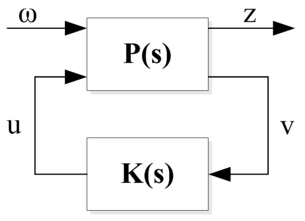
The multivariable robust controller design can be formulated as an H optimization problem based on scheme shown in Figure 8 [21,37]. In this scheme, P(s) is the generalized plant, K(s) is the controller, v the measured variables, u are the control signals, ω are the exogenous signals and z are the error variables.
The controller synthesis is performed according to the systematic design procedure proposed in [37,38]. The optimal H control problem is still unsolved; nevertheless, there are solutions for the suboptimal problem. According to Figure 8, the control problem consists of computing a controller which minimizes the ratio γ between the energy of error variables z and the energy of the exogenous signal vector 
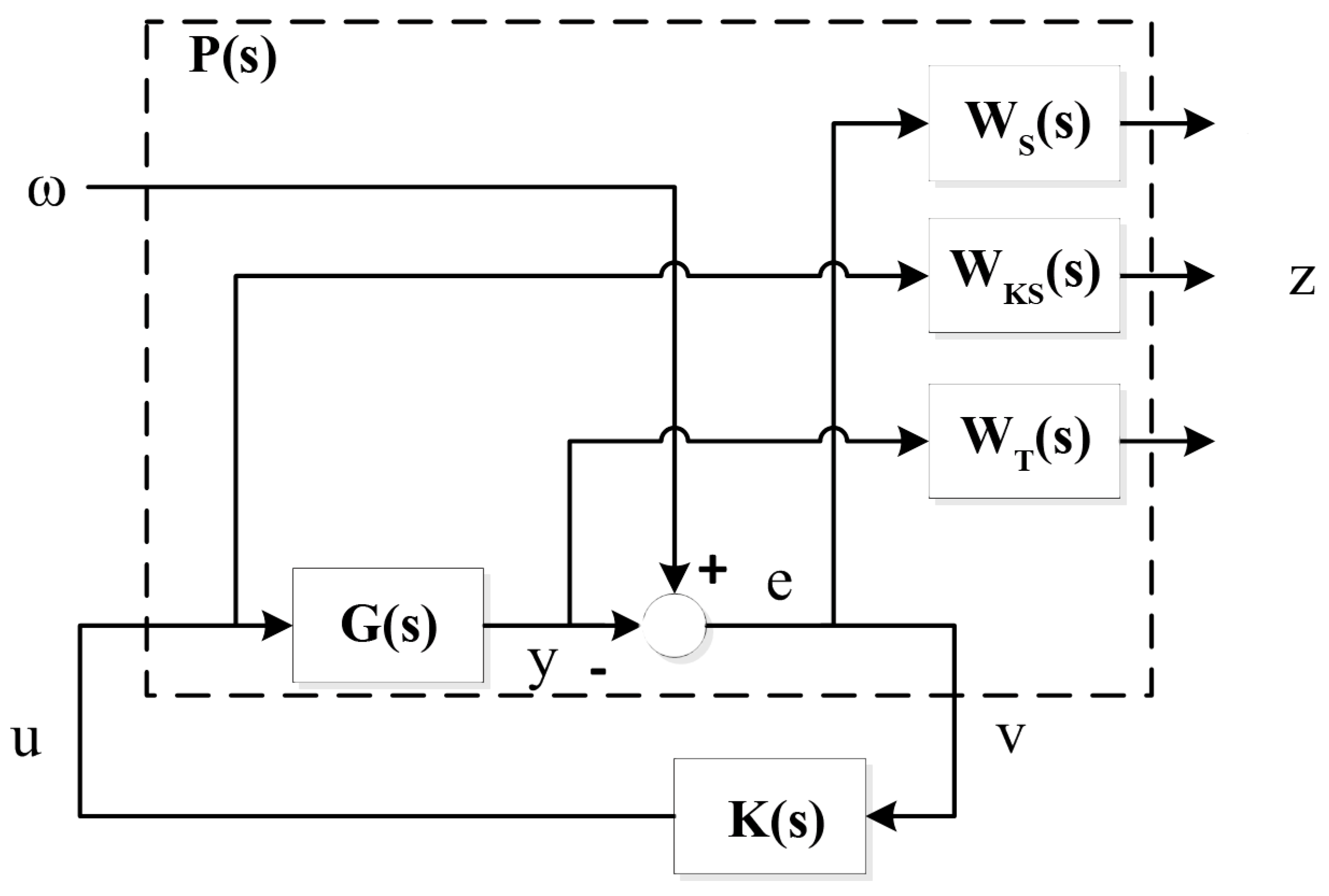
ω. The scheme shown in Figure 9 allows performing the S/KS/T mixed sensitivity problem for developing the generalized plant [21,37]. In this case, the closed loop transfer matrix T(s) is given as follows:
T z ω ( s ) = [ W s ( s ) S o ( s ) W K S ( s ) K ( s ) S o ( s ) W T ( s ) T o ( s ) ] ,
where So(s) is the output sensitivity transfer matrix, To(s) is the output complementary sensitivity transfer matrix, and K(sSo(s) is the control sensitivity transfer matrix. The matrices WS(s), WT(s) and WKS(s) are the corresponding weighting matrices to specify the relevant frequency range for T(s). The choice of these matrices can be carried out by means of design rules.
Next, the design procedure is summarized detailing the different steps [37]. First, the nominal model must be scaled, which is necessary to estimate the multiplicative output uncertainty for the non-nominal models. This multiplicative output uncertainty affects the robust stability (RS) of the system changing the To(s) shape. A proper shape of To(s) is desirable for good reference tracking and noise attenuation. The nominal model can be scaled as follows:
G ^ ( s ) = D e 1 G ( s ) D u ,
where G(s) is the original nominal linear model and De and Du are the scaling matrices.
After obtaining the scaled nominal model, the multiplicative output uncertainty can be estimated according to Equation (12):
E ^ o , i ( s ) = ( G ^ i * ( s ) G ^ ( s ) ) G ^ ( s ) 1 ,
where G ^ i * ( s ) represents the different scaled non-nominal identified models at each operation point.
Next, the matrix WT(s) is defined as a square diagonal matrix as follows:
W T ( s ) = w T d i a g ( s ) × I ,
where wTdiag(s) is a transfer function which must be stable, minimum phase, with high gain at high frequencies and with magnitude greater than the maximum singular value of the uncertainty computed by Equation (12) for each non-nominal model. The matrix WS(s) is designed as the diagonal matrix in Equation (14). Each diagonal element wsi(s) is described according to Equation (15), where ωT is the crossover frequency of wTdiag(s), and αi and βi are the gains at high and low frequencies, respectively. The tuning parameter ki modifies the speed of the output response. This parameter is usually chosen heuristically by trial and error method. The matrix WKS(s) is usually specified as the identity matrix to avoid numerical problems in the synthesis algorithm.
W s ( s ) = [ w s 1 ( s ) 0 0 w s 2 ( s ) ]
w s i ( s ) = α i s + 10 ( k i 1 ) ω T s + β i 10 ( k i 1 ) ω T ,   i = 1 , 2
Finally, after defining the weighting matrices, the controller K ^ (s) is synthesized by using computational software. It is important to remember that the obtained controller is calculated with the scaled plant, so it is necessary to rebuild it as follows:
K ( s ) = D u K ^ ( s ) D e 1 .
For the proposed work, the identified model of the lab-scale wind turbine at wind speed of 8 m/s is used as the nominal model. The scaling matrices are given by Equation (17) and wTdiag(s) has been selected as it is shown in Equation (18).
D e = [ Δ ω r   m a x 0 0 Δ P g   m a x ] = [ 436 0 0 5.86 ] D u = [ Δ β m a x 0 0 Δ α m a x ] = 6 0 0 0.55
w T d i a g ( s ) = 0.5623 ( 50 s + 1 ) ( 0.5 s + 1 )
In the WS(s) matrix, ωT is about 0.0294 rad/s and according to the design process in [37], α1 = α2 = 0.5 and β1 = β2 = 10−4 have been selected. Parameters k1 = 0.15 and k2 = 1.1 have been chosen to achieve similar time responses than those obtained by the previous designs of decoupling methodologies.
The H controller has a ratio γ equal to 7.95. Considering this fact, and according to the condition in Equation (19), this value does not guarantee robust stability. Thus, it is necessary to verify that the sensitivity transfer function and complementary sensitivity transfer functions do not exceed the upper bounded values in the entire range of frequencies [37,38].
T z ω ( s ) = ( W s ( s ) S o ( s ) W K S ( s ) K ( s ) S o ( s ) W T ( s ) T o ( s ) ) < γ
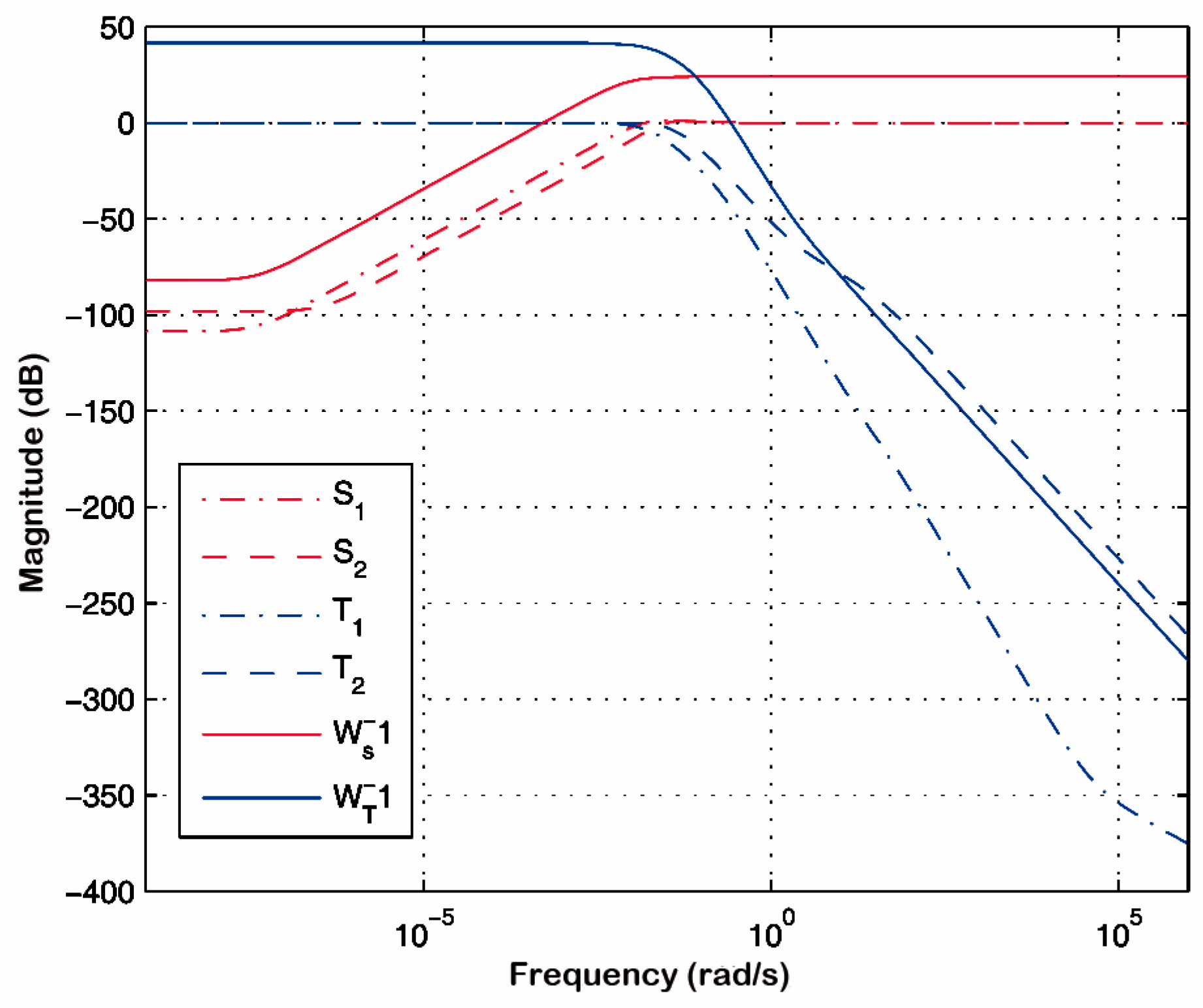
Figure 10 shows the magnitude of the maximum singular value of the diagonal elements of So(s) and To(s), together with the bounded values W S 1 ( s ) and W T 1 ( s ) . It is observed that the maximum singular values of the diagonal elements of the output sensitivity transfer matrix are below of bounded value in the entire frequency range. However, the maximum singular values of the first element of the output complementary sensitivity transfer matrix are above the bounded values at high frequencies.
Usually, the controller K(s) obtained by this procedure has elements with too high order to be implemented. Therefore, the controller is generally reduced e.g., studying the Hankel singular values [39]. Equation (20) shows the second order reduced robust controller matrix.
K ( s ) = ( 0.0009862 s 7.485 10 5 s 2 + 0.09286 s + 1.929 10 9 0.3654 s 0.3371 s 2 + 5.084 s + 9.413 10 7 1.03 10 6 s + 2.986 10 7 s 2 + 0.1043 s + 2.167 10 9 0.000171 s + 4.788 10 5 s 2 + 0.03531 s + 6.538 10 9 )

3.3. Robust Stability Analysis of the Designed Controllers

Next, a robustness evaluation of the proposed decoupling strategies and H controller is performed by means of a 
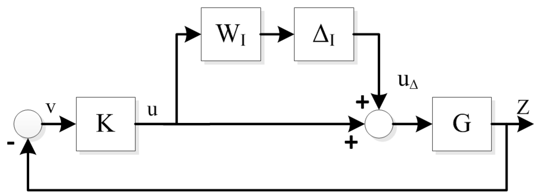
μ-analysis in the presence of diagonal multiplicative input uncertainty. The multiplicative input uncertainty is one of the most difficult to treat in multivariable systems. It is represented as illustrated in Figure 11, where I(s) is the disturbance, and WI(s) is the diagonal uncertainty weight.
The selected weight is given by Equation (21), which can be interpreted as the process inputs increase by up to 150% uncertainty at high frequencies and by almost 15% at low frequencies.
W I ( s ) = w I ( s ) × I = ( 1.5 s + 0.15 ) ( s + 1 ) × I
To achieve robust stability (RS), the necessary and sufficient condition [21] is:
μ R S = μ [ W I ( s ) T I ( s ) ] < 1   ω ,
where μ is the structured singular value (SSV) and TI(s) = K(s)G(s)(I + K(s)G(s))−1 is the input complementary sensitivity function. K(s) is the full centralized control, which is compound of the product D(s)∙C(s) for the case of the proposed decoupling methods.
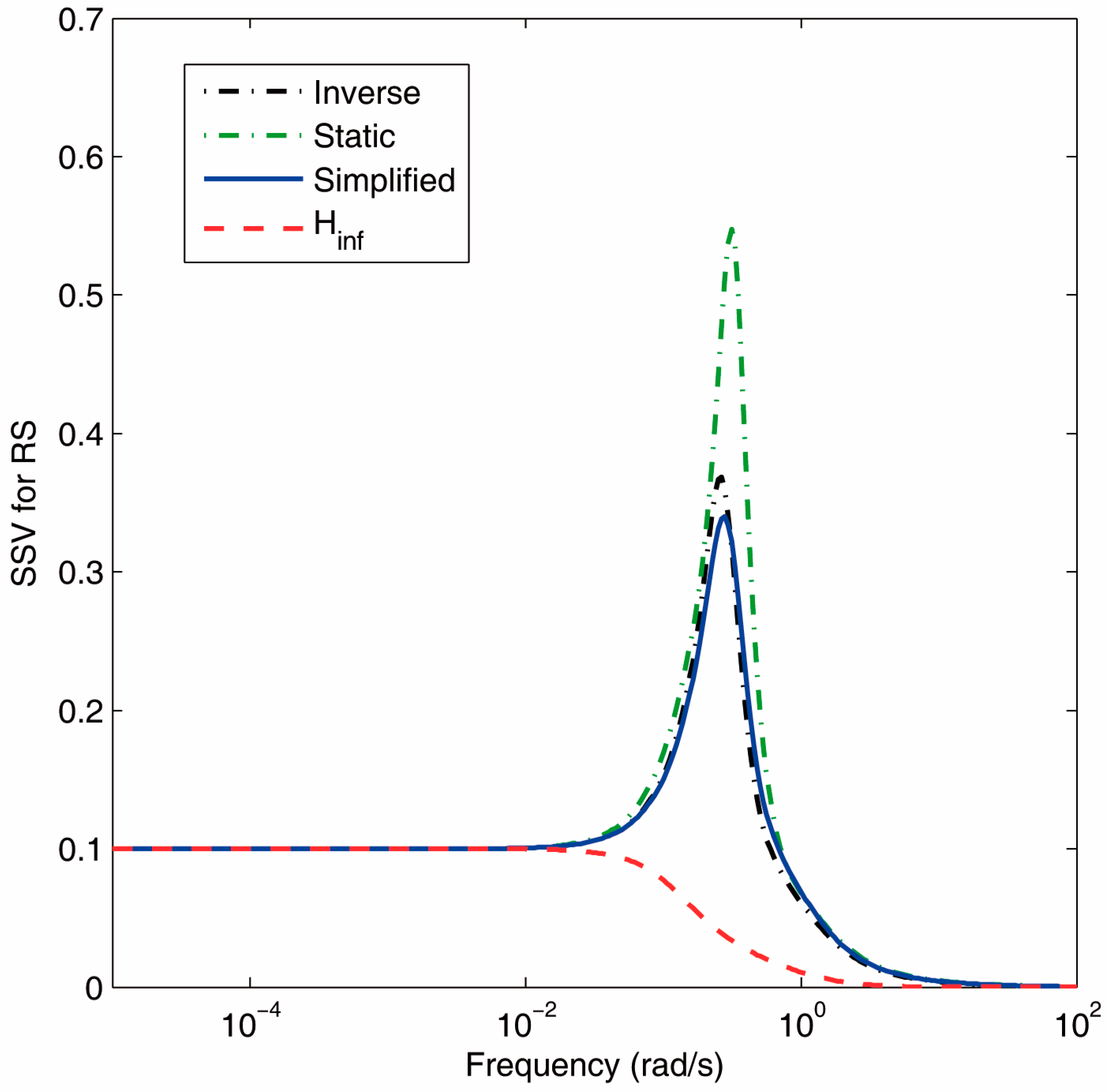
Figure 12 shows the SSV for RS of the different designed controllers. It is observed that the robust control presents the better RS for the entire frequency range, as was expected. Nevertheless, the decoupling strategies fulfill the condition in Equation (28) for all frequencies, which indicates that the system will remain stable despite the process input uncertainty.

4. Simulation and Experimental Results

4.1. Simulation Results

The four proposed controllers described in the previous section are evaluated in simulation. The aim is to illustrate how decoupling techniques can reduce the interaction effect and, consequently, improve the system performance. The first simulation is focused on the transition zone, where the interaction of the lab-scale wind turbine is greater than that shown in the other operation modes, as was demonstrated previously by the RGA analysis. Figure 13 shows the closed-loop responses achieved by the different methods. The initial set-points are 1746 rpm and 6.6 W. At t = 100 s, there is a − 1 W step change in the generated power reference, and at t = 800 s, a − 200 rpm step change occurs in the angular speed reference ωr. Dynamic simplified and inverted decoupling methods obtain perfect decoupling. The H control presents more interaction, above all in the generated power loop. However, it achieves a faster tracking response in this loop.
Next, the same control strategies, which were designed using the identified model around the transition mode, are evaluated in other operational mode, specifically using the model at the full load region with a wind speed of 9 m/s and listed in Table 2. The reference step changes are approximately 15% of the outputs at the corresponding operation point. Figure 14 shows the different closed-loop system responses. The closed-loop performance of the four methodologies is quite similar. However, in this case, no methodology achieves perfect decoupling because the process model has changed.
A quantitative comparison has been established by means of performance indices such as Integral Absolute Error (IAE) and Standard Deviation (Std) for each control loop. Table 5 and Table 6 collect these performance indices for the two performed simulations. Above and below values are the indices for the nominal and non-nominal simulations, respectively. These values indicate that all methodologies achieve similar performance in the ωr loop and that the H control slightly improves the other methodologies in IAE indices of the Pg loop. The inverted decoupling obtains the worst values.
The simulation results with the nominal and non-nominal linear models have demonstrated that the proposed decoupling controllers and H controller achieves a good performance for different operational points and they provide an improvement in the level of interaction between variables. However, the design and implementation of the proposed decoupling controllers are usually easier to perform than the procedure to calculate the H control.

4.2. Experimental Results

The previous simulation results have been also confirmed in the lab-scale VS-VP wind turbine under study in this work. Figure 15 shows the experimental closed-loop response of the lab-scale wind turbine operating at the transition mode with a wind speed profile with mean of 8 m/s and standard deviation of 0.2 m/s. This wind profile is generated using the wind speed model described in Appendix A. There are set point step changes like those of the simulation case.
The results are similar to those obtained in simulation. They point out that no methodology achieves perfect decoupling due to the modeling errors. Nevertheless, the performance achieved by the decoupling control strategies is slightly better than that obtained by the H control, which shows again interaction when the Pg reference changes.
The proposed controllers are also evaluated in the full load operation mode. Figure 16 depicts the corresponding closed-loop responses of the lab-scale wind turbine operating with a wind speed of 9 m/s. There is an acceptable degree of agreement between the simulation and experimental responses. Again, decoupling is no perfect, especially for the rotor speed loop. Nevertheless, decoupling performance is improved in the power loop using the decoupling control strategies in comparison with that achieved by the H control. The blade pitch angle control signal is more degraded with respect to the simulation cases.
Performance can be quantified by several indices, similar to the simulation case. Table 7 summarizes the IAE indices and standard deviations. Above and below values are the indices for the nominal and non-nominal tests, respectively. These indices denote that the H control presents smaller IAE values for the rotor speed loop; however, the decoupling control strategies obtain better results for the rest of the performance indices.

5. Conclusions

In line with the improvement of wind turbine performance by means of its control structure, this work approaches these processes as industrial multivariable multi-model systems and highlights interactions between variables and system uncertainties as main control problems. The VS-VP wind turbines present different dynamic responses depending on the operational mode, and it has been analyzed that the transition zone is the region showing more interaction. The contribution of this work focuses on designing a multivariable controller that can cope with the system interaction at this zone and can achieve a proper performance at other operational modes. A global improvement of the wind turbine response justifies this study. Different decoupling controllers have been developed to deal with those problems. In addition, a robust controller is also designed for comparison since this methodology is specially aimed for processes with great uncertainties.
The methodologies have been tested in simulation and verified experimentally in a lab-scale VS-VP wind turbine. Both techniques achieve a proper response at the design nominal point as well as non-nominal points. In general, all methods show similar performance since they have been designed to do this. At the nominal point, decoupling controllers achieve perfect decoupling while the H control presents important interaction in the generated power loop. At the non-nominal point, none of the methods obtain perfect decoupling; however, the performance of the dynamic simplified decoupling control is quite similar to that of the robust controller. Thus, it has been demonstrated that this proposal can be considered as an appropriate methodology for controlling such systems. The main advantage of the proposed decoupling controllers is the easiness of design and implementation in comparison with the H control procedure. The latter method is complicated to perform, it obtains high order controller elements that are difficult to implement in practice, and, thus, it normally requires a reduction controller procedure. As a disadvantage, decoupling designs must be careful with model uncertainties and must confirm their robust stability.
Future work will be addressed to implement these methodologies in industrial wind turbines. Although this is not straightforward due to the size and technical characteristics of the lab-scale VS-VP wind turbine, it is expected that the main results can be extrapolated. Furthermore, more advanced methodologies such as decoupling control in combination with gain-scheduling can be studied.

Acknowledgments

This work was supported by the Autonomous Government of Andalusia (Spain), under the Excellence Project P10-TEP-6056. This support is gratefully acknowledged.

Author Contributions

Francisco Vázquez and Fernando Morilla conceived and designed the experiments; Sergio Fragoso performed the experiments; Juan Garrido and Francisco Vázquez analyzed the data; and Juan Garrido and Sergio Fragoso wrote the paper.

Conflicts of Interest

The authors declare no conflict of interest. The founding sponsors had no role in the design of the study; in the collection, analyses, or interpretation of data; in the writing of the manuscript, and in the decision to publish the results.

Appendix A

A wind speed model was developed to provide more realistic and precise experiments of the wind turbine output. This wind speed model allowed simulations and experiments in which the wind turbine is subjected to both a variable wind speed profile and a variable reference set-point. The wind speed is a natural phenomenon that can be modeled by a stationary stochastic process that is composed of an average speed vwm, gusts vwg, turbulence vwt and ramps vwr [40].
v w ( t ) = v w m + v w r ( t ) + v w g ( t ) + v w t ( t )
The turbulent component vwt is modeled by the Van der Hoven model [41], as follows:
v w t ( t ) = i = 1 N A i cos ( ω i t + φ i ) ,
A i ( ω i ) = 2 π 1 2 [ S ( ω i ) + S ( ω i + 1 ) ] ( ω i + 1 ω i ) ,
S ( ω ) = 0.475 σ 2 L v w m [ 1 + ( ω L v w m ) 2 ] 5 6 ,
where Ai is the amplitude of the wind speed fluctuation for the discrete frequency ωi (i = [1,n]), which is based on the spectral density function S(ω), where σ represents the standard deviation of the wind speed, L is the length scale of the turbulence, N is the number of samples, and φ i is a random phase angle with a uniform distribution in the range [−π,π]. The ramp component vwr is characterized by three parameters: the ramp amplitude Ar, the start time of the ramp Tsr, and the final time of the ramp Ter. The gust component vwg is also characterized by three parameters: the gust amplitude Ag, the start time of the gust Tsg, and the final time of the gust Teg.

References

  1. Fragoso, S.; Garrido, J.; Vázquez, F.; Morilla, F. Comparative analysis of decoupling control methodologies and H multivariable robust control for VS-VP wind turbines. In Proceedings of the IREC2015 the Sixth International Renewable Energy Congress, Sousse, Tunisia, 24–26 March 2015. [Google Scholar]
  2. Simani, S. Overview of Modelling and Advanced Control Strategies for Wind Turbine Systems. Energies 2015, 8, 13395–13418. [Google Scholar] [CrossRef]
  3. Bossanyi, E.A. The design of closed loop controllers for wind turbines. Wind Energy 2000, 3, 149–163. [Google Scholar] [CrossRef]
  4. Van der Hooft, E.L.; van Engelen, T.G. Estimated wind speed feed forward control for wind turbine operation optimisation. In Proceedings of the European Wind Energy Conference, London, UK, 22–25 November 2004. [Google Scholar]
  5. Pao, L.Y.; Johnson, K.E. A tutorial on the dynamics and control of wind turbines and wind farms. In Proceedings of the 2009 American Control Conference, St. Louis, MO, USA, 10–12 June 2009; pp. 2076–2089. [Google Scholar]
  6. Wu, F.; Zhang, X.; Member, S.; Ju, P.; Sterling, M.J.H. Decentralized Nonlinear Control of Wind Turbine with Doubly Fed Induction Generator. IEEE Trans. Power Syst. 2008, 23, 613–621. [Google Scholar]
  7. Simoes, M.G.; Bose, B.K.; Spiegel, R.J. Fuzzy Logic Based Intelligent Control of a Variable Speed Cage Machine Wind Generation System. IEEE Trans. Power Electron. 1997, 12, 87–95. [Google Scholar] [CrossRef]
  8. Badihi, H.; Zhang, Y.; Hong, H. Wind turbine fault diagnosis and fault-tolerant torque load control against actuator faults. IEEE Trans. Control Syst. Technol. 2015, 23, 1351–1372. [Google Scholar] [CrossRef]
  9. Li, H.; Shi, K.L.; McLaren, P.G. Neural-Network-Based Sensorless Maximum Wind Energy Capture with Compensated Power Coefficient. IEEE Trans. Ind. Appl. 2005, 41, 1548–1556. [Google Scholar] [CrossRef]
  10. Assareh, E.; Biglari, M. A novel approach to capture the maximum power from variable speed wind turbines using PI controller, RBF neural network and GSA evolutionary algorithm. Renew. Sustain. Energy Rev. 2015, 51, 1023–1037. [Google Scholar] [CrossRef]
  11. Yang, X.; Xu, L.; Liu, Y.; Xu, D. Multivariable Predictive Functional Control for Doubly Fed Induction Generator. In Proceedings of the IEEE International Conference on Control and Automation, Guangzhou, China, 30 May–1 June 2007. [Google Scholar]
  12. Jain, A.; Schildbach, G.; Fagiano, L.; Morari, M. On the design and tuning of linear model predictive control for wind turbines. Renew. Energy 2015, 80, 664–673. [Google Scholar] [CrossRef]
  13. Rocha, R.; Filho, L.S.M. A multivariable H∞ control for wind energy conversion system. In Proceedings of the 2003 IEEE Conference on Control Applications, Istambul, Turkey, 23–25 June 2003; pp. 206–211. [Google Scholar]
  14. Selvam, K.; Kanev, S.; Van Wingerden, J.W.; Van Engelen, T. Feedback-Feedforward Individual Pitch Control for Wind Turbine Load Reduction. Int. J. Robust Nonlinear Control 2009, 19, 72–91. [Google Scholar] [CrossRef]
  15. Imran, R.M.; Akbar Hussain, D.M.; Chen, Z. LQG controller design for pitch regulated variable speed wind turbine. In Proceedings of the IEEE International Energy Conference (ENERGYCON), Dubrovnik, Croatia, 13–16 May2014; pp. 101–105. [Google Scholar]
  16. Østergaard, K.Z.; Stoustrup, J.; Brath, P. Linear Parameter Varying Control of Wind Turbines Covering both Partial Load and Full Load Conditions. Int. J. Robust Nonlinear Control 2009, 19, 92–116. [Google Scholar] [CrossRef]
  17. Cao, G.; Grigoriadis, K.M.; Nyanteh, Y.D. LPV control for the full region operation of a wind turbine integrated with synchronous generator. Sci. World J. 2015, 2015, 638120. [Google Scholar] [CrossRef] [PubMed]
  18. Boukhezzar, B.; Siguerdidjane, H. Nonlinear control of variable speed wind turbines for power regulation. In Proceedings of the IEEE Conference on Control Applications, Toronto, ON, Canada, 28–31 August 2005; pp. 114–119. [Google Scholar]
  19. Boukhezzar, B.; Lupu, L.; Siguerdidjane, H.; Hand, M. Multivariable control strategy for variable speed, variable pitch wind turbines. Renew. Energy 2007, 32, 1273–1287. [Google Scholar] [CrossRef]
  20. Morilla, F.; Garrido, J.; Vázquez, F. Multivariable Control by Decoupling. Rev. Iberoam. Autom. Inform. Ind. 2013, 10, 3–17. [Google Scholar] [CrossRef]
  21. Skogestad, S.; Postlethwaite, I. Multivariable Feedback Control: Analysis and Design, 2nd ed.; John Wiley & Sons: Chichester, UK, 2005. [Google Scholar]
  22. Fragoso, S.; Ruz, M.L.; Garrido, J.; Vázquez, F.; Morilla, F. Educational software tool for decoupling control in wind turbines applied to a lab-scale system. Comput. Appl. Eng. Educ. 2016, 24, 400–411. [Google Scholar] [CrossRef]
  23. Bianchi, F.; De Battista, H.; Mantz, R. Wind Turbine Control Systems: Principles, Modelling and Gain Scheduling Design; Springer: London, UK, 2007. [Google Scholar]
  24. Anaya-Lara, O.; Jenkins, N.; Ekanayake, J.; Cartwright, P.; Hughes, M. Wind Energy Generation: Modelling and Control; John Wiley & Sons: Chichester, UK, 2009. [Google Scholar]
  25. García-Sanz, M.; Torres, E. Control y Experimentación del Aerogenerador Síncrono de Velocidad Variable TWT1650. Rev. Iberoam. Autom. Inform. Ind. 2004, 1, 53–62. [Google Scholar]
  26. Dodson, L.; Busawon, K.; Jovanovic, M. Estimation of the power coefficient in a wind conversion system. In Proceedings of the 44th IEEE Conference on Decision and Control and the European Control Conference, Seville, Spain, 12–15 December 2005; pp. 3450–3455. [Google Scholar]
  27. Van der Veen, G.J. Identification of Wind Energy Systems. Ph.D. Thesis, Delft Technical University, Delft, The Netherlands, 2013. [Google Scholar]
  28. Bristol, E.H. On a New Measure of Interaction for Multivariable Process. IEEE Trans. Autom. Control 1966, 11, 133–134. [Google Scholar] [CrossRef]
  29. Wang, Q.W. Decoupling Control; Lectures Notes in control and Information Sciences 285; Springer: Berlin, Germany, 2003. [Google Scholar]
  30. Waller, K. Decoupling in distillation. AIChE J. 1974, 20, 592–594. [Google Scholar]
  31. Åström, K.J.; Johansson, K.H.; Wang, Q.W. Design of decoupled PI controller for two-by-two systems. IEE Proc. Control Theory Appl. 2002, 149, 74–81. [Google Scholar] [CrossRef]
  32. Cai, W.J.; Ni, W.; He, M.J.; Ni, C.Y. Normalized decoupling—A new approach for MIMO process control system design. Ind. Eng. Chem. Res. 2008, 47, 7347–7356. [Google Scholar] [CrossRef]
  33. Wade, H.L. Inverted decoupling: A neglected technique. ISA Trans. 1997, 36, 3–10. [Google Scholar] [CrossRef]
  34. Garrido, J.; Vázquez, F.; Morilla, F.; Hagglund, T. Practical Advantages of Inverted Decoupling. Proc. Inst. Mech. Eng. I J. Syst. Control Eng. 2011, 225, 977–992. [Google Scholar] [CrossRef]
  35. Morilla, F.; Dormido, S. Methodologies for the tuning of PID controllers in the frequency domain. In Proceedings of the IFAC Workshop on Digital Control, Past, Present and Future of PID Control, Terrassa, Spain, 5–7 April 2000; pp. 155–160. [Google Scholar]
  36. Vázquez, F.; Morilla, F.; Dormido, S. An Iterative Method for Tuning Decentralized PID Controllers. In Proceedings of the 14th IFAC World Congress, Beijing, China, 5–9 July 1999; pp. 491–496. [Google Scholar]
  37. Ortega, M.G.; Rubio, F.R. Systematic design of weighting matrices for the H∞ mixed sensitivity problem. J. Process Control 2004, 14, 89–98. [Google Scholar] [CrossRef]
  38. Ortega, M.G.; Castaño, F.; Vargas, M.; Rubio, F.R. Multivariable robust control of a rotary dryer: Analysis and design. Control Eng. Pract. 2007, 15, 487–500. [Google Scholar] [CrossRef]
  39. Boyd, S.; El Ghaoui, L.; Feron, E.; Balakirshman, V. Linear Matrix Inequalities in System and Control Theory; Society for Industrial and Applied Mathematics (SIAM): Philadelphia, PA, USA, 1994. [Google Scholar]
  40. Barakati, S.M. Modeling and Controller Design of a Wind Energy Conversion System Including a Matrix Converter. Ph.D. Thesis, University of Waterloo, Waterloo, ON, Canada, 2008. [Google Scholar]
  41. Van der Hoven, I. Power Spectrum of Horizontal Wind Speed in the Frequency Range from 0.0007 to 900 Cycles per Hour. J. Atmos. Sci. 1957, 14, 160–164. [Google Scholar] [CrossRef]
Figure 1. Wind turbine operation modes.
Sustainability 09 00713 g001
Figure 2. Multivariable control scheme.
Sustainability 09 00713 g002
Figure 3. Lab-scale small wind turbine.
Sustainability 09 00713 g003
Figure 4. Polynomial fitting of the power coefficient C p ( λ , β ) in four cases of constant pitch angle.
Sustainability 09 00713 g004
Figure 5. Experimental power coefficient C p ( λ , β ) surface.
Sustainability 09 00713 g005
Figure 6. Relative step responses of the experimental system (solid line) and the identified model (dashed-dotted line) for a wind speed of 8 m/s.
Sustainability 09 00713 g006
Figure 7. Decoupling control system of a TITO process: (a) conventional decoupling; and (b) inverted decoupling.
Sustainability 09 00713 g007
Figure 8. General formulation of the control problem.
Sustainability 09 00713 g008
Figure 9. S/KS/T mixed sensitivity configuration.
Sustainability 09 00713 g009
Figure 10. Diagonal elements of S o ( s ) and T o ( s ) and the upper bounded values.
Sustainability 09 00713 g010
Figure 11. System with multiplicative input uncertainty.
Sustainability 09 00713 g011
Figure 12. SSV for RS.
Sustainability 09 00713 g012
Figure 13. Outputs and control signals of the simulated closed-loop with the nominal model in the transition mode at wind speed 8 m/s.
Sustainability 09 00713 g013
Figure 14. Outputs and control signal of the simulated closed-loop with the non-nominal model in the full load mode at wind speed 9 m/s.
Sustainability 09 00713 g014
Figure 15. Outputs and control signals of the experimental closed-loop in the transition mode at wind speed 8 m/s.
Sustainability 09 00713 g015
Figure 16. Outputs and control signals of the experimental closed-loop in the full load mode at wind speed 9 m/s.
Sustainability 09 00713 g016
Table 1. Technical parameters of the small experimental wind turbine.
ParameterValue
Rotor radius ( R ) 297.5 mm
Rated power ( P g r ) 80 W
Rated speed ( ω r r ) 1810 rpm (189.5 rad/s)
Rated voltage ( U g r ) 24 V
Rated current ( I g r ) 2.94 A
Rotor inertia ( J r ) 11000 g·cm2
Generator inertia ( J g ) 1340 g·cm2
Armature resistance ( R a ) 1.44 Ω
Armature inductance ( L a ) 0.56 mH
Speed constant ( k b ) 95.3 rpm/V
Torque constant ( k t ) 100 mNm/A
Efficiency ( η ) 77%
Load resistance ( R L ) 22 Ω (100 W)
Table 2. Resulting linear models.
Wind Speed G ( s ) G D ( s )
6 m/s ( 8.059 75.27 s 2 + 17.35 s + 1 405.4 28.25 s 2 + 16.47 s + 1 0.0081479 16.873 s + 1 4.4195 1.7589 s + 1 ) ( 364.9 118.3 s 2 + 21.76 s + 1   1.139 65.28 s 2 + 17.09 s + 1   )
7 m/s ( 10.534 97.41 s 2 + 20.63 s + 1   520.3 16.61 s 2 + 15.81 s + 1   0.039756 14.653 s + 1   5.8011 1.2295 s + 1   ) ( 340.01 110.3 s 2 + 21.01 s + 1   1.139 52.72 s 2 + 14.97 s + 1   )
8 m/s ( 8.3951 118.4 s 2 + 21.77 s + 1   491.4 35.36 s 2 + 11.89 s + 1   0.06102 16.93 s + 1 6.7614 0.93526 s + 1 ) ( 345 104.6 s 2 + 20.45 s + 1 2.341 41.53 s 2 + 14.85 s + 1 )
9 m/s ( 45.251 113.4 s 2 + 21.37 s + 1   366.8 50.86 s 2 + 14.36 s + 1   0.3132 16.803 s + 1   8.0643 1.10434 s + 1   ) ( 287.46 85.1 s 2 + 18.45 s + 1   2.0273 40.73 s 2 + 12.76 s + 1   )
10 m/s ( 59.06 116.8 s 2 + 21.62 s + 1   300.6 0.01389 s 2 + 13.9 s + 1 0.3932 16.395 s + 1   8.6291 1.446 s + 1   ) ( 248.2 74.04 s 2 + 17.21 s + 1   1.791 21.91 s 2 + 11.91 s + 1   )
Table 3. RGA of the models.
Wind Speed λ 11 RGA
6 m/s 0.9151
7 m/s 0.7471
8 m/s 0.6543
9 m/s 0.7606
10 m/s 0.8118
Table 4. Expressions for different decoupling networks and corresponding apparent processes.
Decoupling Scheme D ( s ) Q ( s )
Ideal ( g 11 ( s ) g 22 ( s ) g 12 ( s ) g 22 ( s ) g 11 ( s ) g 21 ( s ) g 11 ( s ) g 22 ( s ) ) g 11 ( s ) g 22 ( s ) g 12 ( s ) g 21 ( s ) ( g 11 ( s ) 0 0 g 22 ( s ) )
Simplified ( 1 g 12 ( s ) g 11 ( s ) g 21 ( s ) g 22 ( s ) 1 ) ( g 11 ( s ) g 12 ( s ) g 21 ( s ) g 22 ( s ) 0 0 g 22 ( s ) g 12 ( s ) g 21 ( s ) g 11 ( s ) )
Inverted d 12 ( s ) = g 12 ( s ) g 11 ( s )   d 21 ( s ) = g 21 ( s ) g 22 ( s ) ( g 11 ( s ) 0 0 g 22 ( s ) )
Table 5. Designed decoupling elements for the nominal model of lab-scale wind turbine.
Decoupling Scheme D ( s )
Dynamic simplified ( 1 196 s 2 36.04 s 1.655 s 2 + 0.34 s + 0.028 0.00049 s + 0.00053 s + 0.059 1 )
Static simplified ( 1 58.5341 0.00902 1 )
Inverted d 12 ( s ) = 196 s 2 36.04 s 1.655 s 2 + 0.34 s + 0.028  
d 21 ( s ) = 0.00049 s + 0.00053 s + 0.059
Table 6. Simulation performance indices.
Method I A E 1 I A E 2 S t d 1 S t d 2
H 1.35 × 1061.28 × 10495.460.369
6.45 × 1057.21 × 10347.290.272
Dynamic simplified1.36 × 1066.15 × 10395.680.316
5.85 × 1055.25 × 10347.530.260
Static simplified1.41 × 1067.17 × 10395.350.319
5.85 × 1055.28 × 10347.390.261
Inverted2.07 × 1069.40 × 10392.650.316
8.94 × 1058.01 × 10346.020.267
Table 7. Experimental performance indices.
Method I A E 1 I A E 2 S t d 1 S t d 2
H 1.88 × 104243.8888.820.474
2.25 × 104244.5986.860.464
Dynamic simplified2.24 × 104106.0387.810.387
3.59 × 10499.86107.010.386
Static simplified2.96 × 10499.8485.570.387
3.78 × 104115.04104.050.390
Inverted3.15 × 104132.8982.030.392
5.11 × 104135.4098.460.396

