Article

Spatiotemporal Dynamics and Spatial Determinants of Urban Growth in Suzhou, China

1
Department of Geography, University of Utah, Salt Lake City, UT 84112, USA
2
Department of Land Management, Zhejiang University, Hangzhou 310029, China
3
Environmental and Climate Sciences Department, Brookhaven National Laboratory, Upton, NY 11973, USA
*
Author to whom correspondence should be addressed.
Sustainability 2017, 9(3), 393; https://doi.org/10.3390/su9030393
Submission received: 2 January 2017 / Revised: 28 February 2017 / Accepted: 1 March 2017 / Published: 7 March 2017
(This article belongs to the Section Sustainable Urban and Rural Development)

Abstract

:
This paper analyzes the spatiotemporal dynamics of urban growth and models its spatial determinants in China through a case study of Suzhou, a rapidly industrializing and globalizing city. We conducted spatial analysis on land use data derived from multi-temporal remote sensing images of Suzhou from 1986 to 2008. Three urban growth types, namely infilling, edge-expansion, and leapfrog, were identified. We used landscape metrics to quantify the temporal trend of urban growth in Suzhou. During these 22 years, Suzhou’s urbanization changed from bottom-up rural urbanization to city-based top-down urban expansion. The underlying mechanism changed from TVE (town village enterprise) driven rural industrialization to FDI (foreign direct investment) driven development zone fever. Furthermore, we employed both global and local logistic regressions to model the probability of urban land conversion against a set of spatial variables. The global logistic regression model found the significance of proximity, neighborhood conditions, and socioeconomic factors. The logistic geographically weighted regression (GWR) model improved the global regression model with better model goodness-of-fit and higher prediction accuracy. More importantly, the local parameter estimates of variables enabled us to exam spatial variations of the influences of variables on urban growth in Suzhou.

1. Introduction

Since the launch of economic reforms and open-door policies in 1978, China has experienced unprecedented urbanization. Tremendous urban land expansion has taken place in Chinese cities and regions [1,2,3]. By the end of 2011, for the first time in the history of China, more Chinese people lived in cities and towns than in the countryside [4]. However, the rapid urbanization in China is also accompanied by arable land loss, landscape fragmentation, and sustainability challenges [1,5,6]. Many efforts have been made to analyze the complex pattern of urban land expansion and understand the underlying factors [7,8,9].
Urban growth in China has been studied from different perspectives. Scholars have managed to understand the driving forces of urban land expansion in China from institutional and political economy perspectives [10,11,12,13,14]. They find that urban growth in China is driven by economic reforms and globalization and led by the state and transnational corporations. With the advances in spatial modeling, geographic information systems (GIS), and remote sensing, various models have been developed to analyze urban growth patterns in China. Among them, neural-network-based cellular automata models and agent-based models are usually used to predict/simulate land use change scenarios [15,16,17]. Nevertheless, these models are often inadequate to incorporate socioeconomic factors in explaining underlying mechanisms and diverse patterns of urban growth.
Previous urban expansion models tend to reveal urban growth patterns from a global view, which assumes that the influence of various factors can be applied uniformly throughout the whole study area with little consideration of spatial variation. However, urban growth is a nonstationary process over space. The importance of spatial heterogeneity in land use change should not be overlooked [18]. A few recent studies have taken account of the spatial nonstationary relationship between urban growth and explanatory factors by using spatially explicit models such as geographical weighted regression (GWR) and spatial expansion methods [8,9,19].
Through a case study of Suzhou City in the Yangtze River Delta, this study aims to examine the spatiotemporal dynamics of urban growth in Suzhou by using spatial analysis, GIS, and landscape metrics and incorporating institutional analysis. Moreover, by employing the logistic GWR model, this research investigates the spatially varying relationship between urban land conversion and underlying factors. Lastly, the case of Suzhou, a second-tier city different from the largest national centers, can help improve the understanding of the diverse patterns and determinants of urban growth in China.

2. Data and Methods

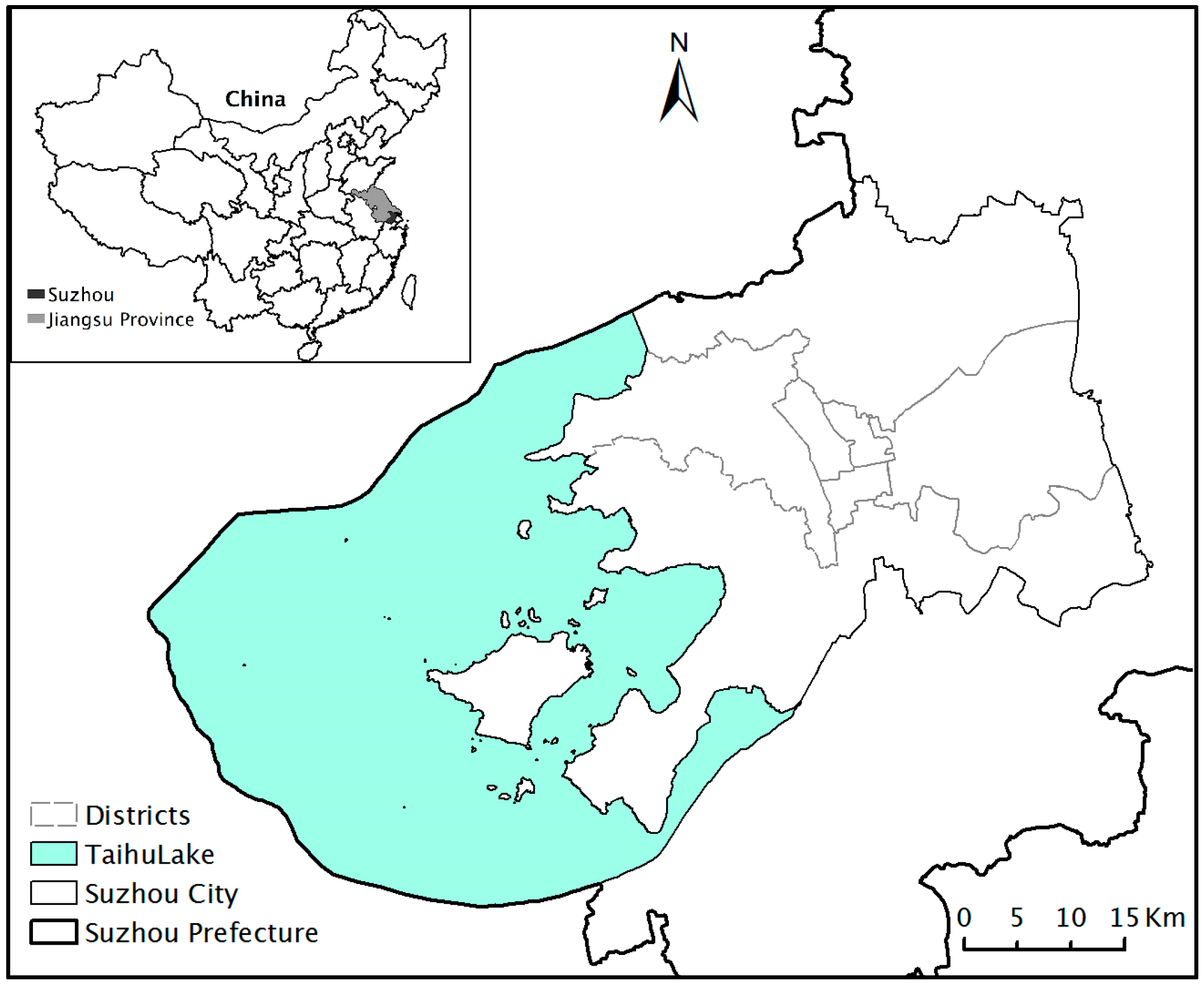
2.1. Study Area and Data

2.1.1. Study Area

Suzhou has a history of more than 2500 years. It is one of the ancient capitals and historical cities of China. Located in southern Jiangsu Province (Sunan) of East China (Figure 1), the city is situated on the eastern shore of Taihu Lake and the lower reaches of the Yangtze River Delta. Suzhou is well known for its beautiful scenery, especially its classic gardens, waters, and bridges, and has been dubbed the Venice of the East. It is crisscrossed with numerous rivers, canals, and lakes. The average elevation of Suzhou is only about 4 m, but there are low mountains distributed in the west of the city. Suzhou has a long history of agricultural development with its advantages in water, climate, and soil, and was once a major rice production base of China.
Suzhou had been the economic and cultural core of the Yangtze River Delta since the Song Dynasty. It was the national center of manufacture and commerce in the Ming and Qing Dynasties [20]. However, in the mid-19th century, Suzhou began to stagnate because of the penetration of colonial forces and the devastating Taiping Rebellion. Its status was gradually replaced by Shanghai, a booming treaty port. Since the economic reform in 1978, Suzhou has experienced rapid economic growth, boosting its GDP to 670 billion yuan in 2008, and ranked the fifth in the nation. During the 1980s, local state-directed township and village enterprises (TVEs) blossomed in Sunan and created a successful pathway of development known as the Sunan Model [21]. In the early 1990s, Suzhou began to learn from the experiences of successful development zones and their strategies of attracting foreign direct investment (FDI). Since the mid-1990s, Suzhou has moved away from the orthodox Sunan Model towards globalization and has emerged as a hot manufacturing center and a major FDI destination in China [20].
Suzhou City is the prefectural seat of Suzhou Prefecture, which also includes five other county-level cities. The administrative division of Suzhou Prefecture has been changing since the 1980s, and Suzhou City has been annexing land from neighboring cities. To maintain consistency for analysis, we use the administrative division of Suzhou City in 2008, when it consisted of seven districts (Figure 1). At the end of 2010, this city covered an area of 1810 km2 with a population of 4 million.

2.1.2. Data

Satellite remote sensing data can provide accurate and timely geospatial information for monitoring land use change. We used five Landsat Thematic Mapper(TM) images (Path 119/Row 38) from 1986, 1991, 1995, 2002, and 2008 for this research. These images were all downloaded from the website of the United States Geological Survey (USGS, http://earthexplorer.usgs.gov/). We also used other spatial data such as a digital elevation model (DEM), GIS files of the transportation network (2006), administrative divisions (2008), and socioeconomic data from statistical yearbooks (1991–2009). These data were provided by the Nanjing Institute of Geography and Limnology, the Suzhou Statistic Bureau, and the Suzhou Planning Bureau.

2.2. Methods

2.2.1. Land Use Data Sampling

The land use data employed in this study were derived from five Landsat TM images (30 m × 30 m resolution). Specifically, we used a machine learning algorithm Random Forest, developed by Breiman [22] and implemented in R by Liaw and Wiener [23], to ‘train’ the computer system to do supervised classification. Then we selected 500 points from each classified image using stratified random sampling and compared them with reference data (high-resolution images or GIS land-cover data). The overall accuracy varied from year to year, but all of them were higher than 85%. Four types of land use were classified; water, wetland, vegetated, and built-up. In this research, urban land is defined in a broad sense as the built-up area in the classified images.
To extract the nonurban to urban land use conversion area, a spatial overlay operation was performed between two classified images in 1991 and 2008. The image for urban land expansion has 2318 × 2059 pixels, a huge dataset that is difficult to handle, and a proper sampling method is required. To reduce the spatial dependence and ensure that the sample represents the population, we used a spatial sampling method combining systematical sampling and random sampling [8,24]. First, we extracted regularly spaced points with a 10-pixel (300 m) interval from the nonurban areas in the 1991 image. Then, from this result, we extracted all 2409 points with nonurban to urban land use conversion. Lastly, we randomly selected another set of 2409 points from those without urban land conversion and got a total of 4818 sample points. Such a sample size well represents the population and can be handled by most statistical software.

2.2.2. Selection of Landscape Metrics

Originally developed in the study of landscape ecology, landscape metrics have been recently applied to urban morphology [25,26]. Landscape metrics can be defined at the patch, class (patch type), and landscape level. A variety of landscape metrics have been developed to describe the proportion of landscape with a particular land cover class; the size, number, perimeter, and the complexity of shape of the patch in that class [27]. Many empirical studies have employed these indices to assess the fragmentation of urban land use [28,29]. In this study, we selected the following landscape metrics, defined at the class level, to analyze the overall changes in urban land patterns; number of patches (NP), largest patch index (LPI), edge density (ED), mean patch size (MPS), area-weighted mean patch fractal dimension (AWMPFD), and area-weighted mean Euclidean nearest-neighbor distance (AWMENND) (see Table 1). All the indices were calculated using the public domain software FRAGSTATS version 4.2 [27].

2.2.3. Type of Urban Growth

For the convenience of implementation, we used a simple equation to distinguish three types of newly developed urban land patches, proposed by Xu et al. [30].
S = L c P
where Lc is the length of the common boundary of a newly developed urban patch and the pre-growth urban patches, and P is the perimeter of the newly grown patch. Urban growth type is defined as infilling when S ≥ 0.5, edge-expansion when 0 < S < 0.5, and leapfrog growth when S = 0, which indicates no common boundary [30].

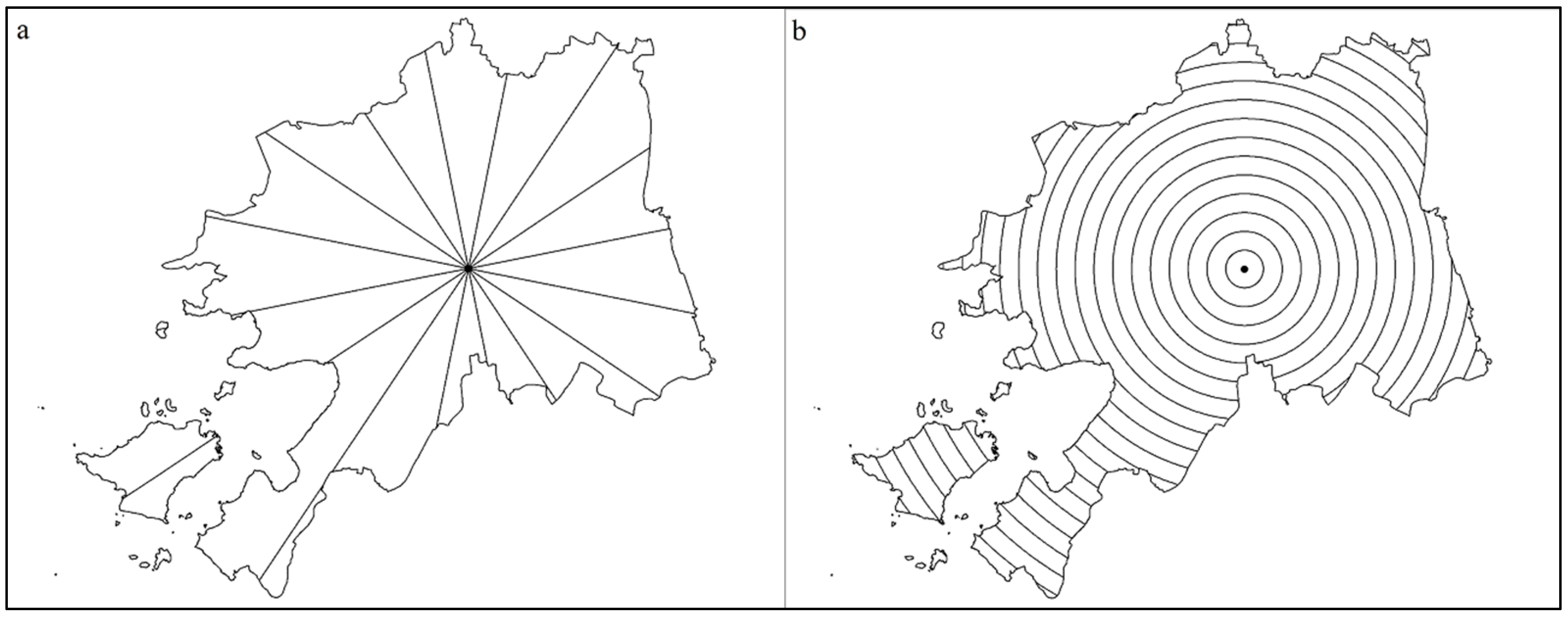
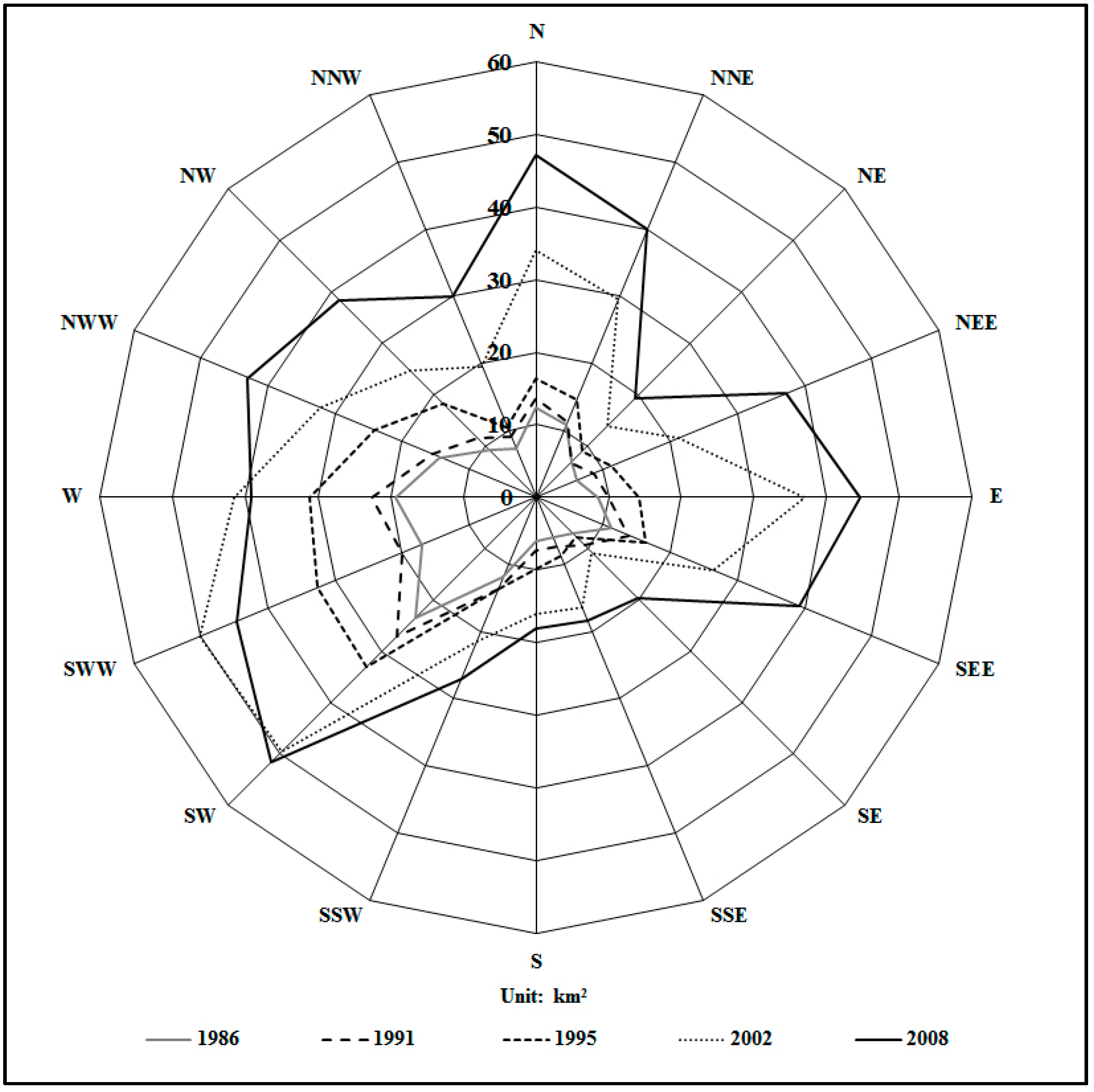
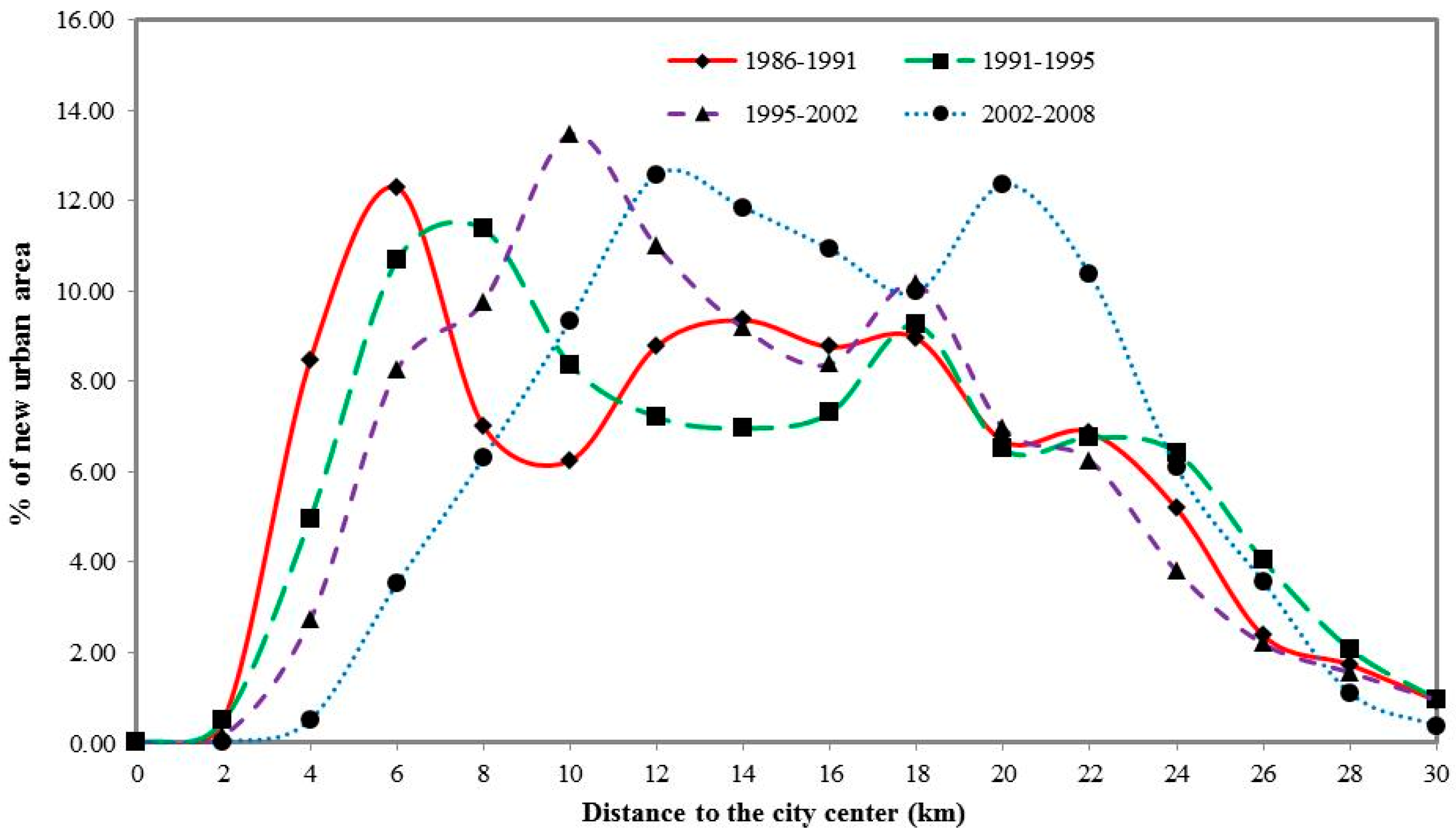
2.2.4. Sector and Concentric Circle Analyses

Sector and concentric circle analyses were employed to characterize the spatiotemporal dynamics of urban land expansion in Suzhou (Figure 2). The sector analysis was used to characterize the quantity and spatial distribution of urban land in terms of angular orientation relative to a predetermined urban center [31]. We drew 16 directional axes from the urban center to form 16 sectors (fan-shaped areas), each having an angle of 22.5 degrees. Then we overlaid these fan-shaped sectors with land use data and calculated the area of urban land within each sector. These values were displayed on the corresponding directional axes to show the spatial distribution of urban land in the city. The concentric circle analysis was used for analyzing the relationship between the area of urban growth and the distance from the urban center. A total of 15 concentric circles were created, each having a width of two kilometers. Then we overlaid these concentric zones with newly grown urban land in each time period and calculated the percentage of urban growth area within each zone.

2.2.5. Logistic Regression Model

The logistic regression model has been widely used to analyze the determinants of urban land conversion. Applying the model to land use change in Guangzhou, China, Wu and Yeh [32] find that road accessibility and socioeconomic factors are the important determinants of urban land development in a transitional economy. Verburg et al. [33] use this model to analyze land use change in the Netherlands and find that the expansions of residential, industrial/commercial, and recreational areas can be explained by a combination of accessibility measures, spatial policies, and neighborhood interaction.
In this research, we also adopted the logistic regression model to identify the determinants of urban growth in Suzhou. The dependent variable Y of the logistic regression was a presence or absence event, when Y = 1 it means a pixel converted from nonurban to urban land, and Y = 0 otherwise. P (Y = 1) means the probability of nonurban to urban land conversion. The logistic regression model is described as [8,24]
logit   ( Y ) = β 0 + k = 1 n β k X k + ε
where X k are independent variables and logit( Y ) is a linear combination function of the independent variables; β 0 is the constant; parameter β k is the regression coefficient of independent variable X k to be estimated; and ε is the error term. The logit ( Y ) can be transformed back to the probability that ( Y = 1)
P   ( Y = 1 ) = exp ( β 0 + k = 1 n β k X k ) 1 + exp ( β 0 + k = 1 n β k X k )

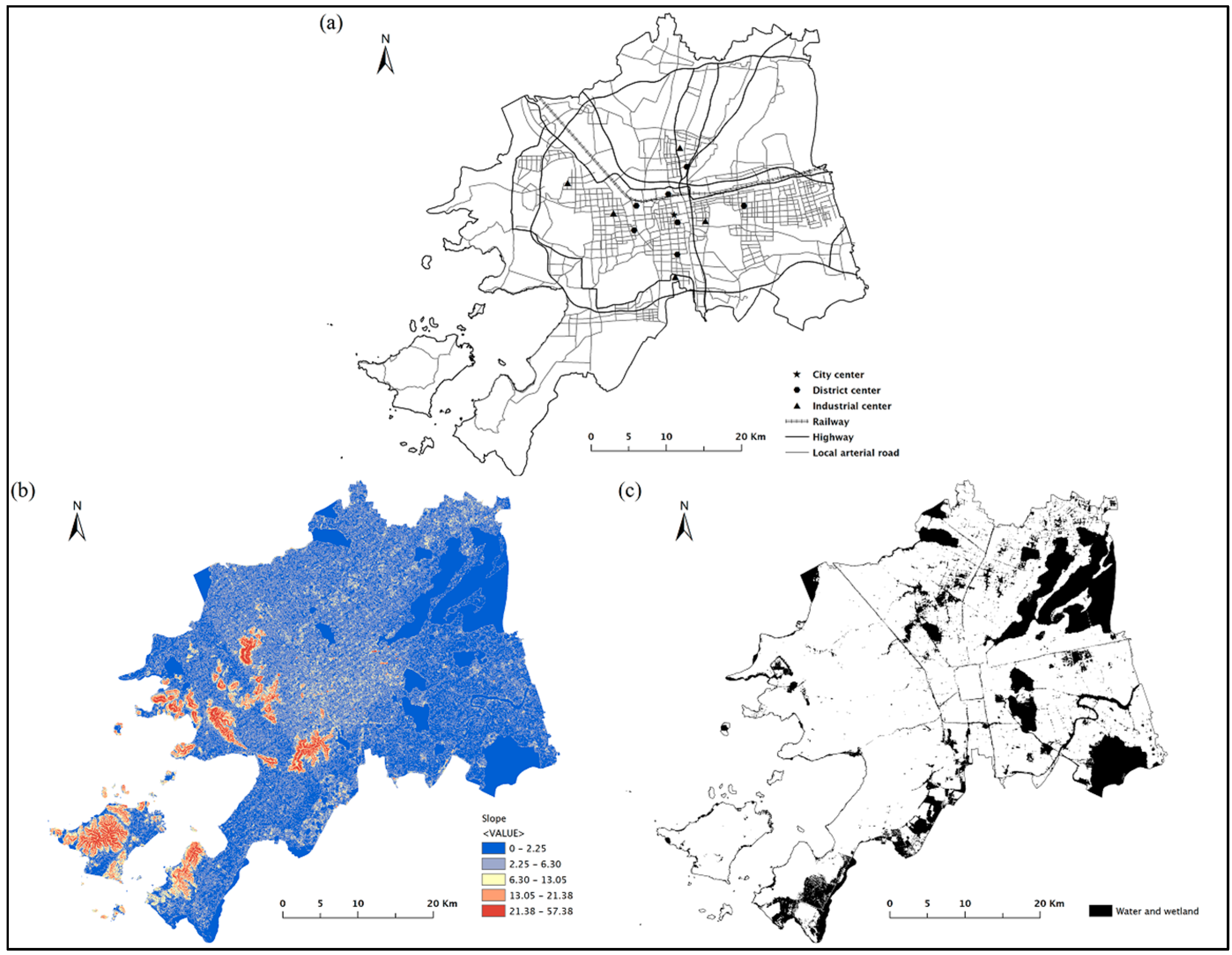
2.2.6. Specification of Dependent and Independent Variables

As mentioned above, the dependent variable is a presence or absence event, when Y = 1 means a pixel converted from nonurban to urban land during the period from 1991 to 2008 and Y = 0 means the pixel remained as nonurban land. Many types of explanatory factors have been identified in land use conversion models, including accessibility to road infrastructure, attributes of neighborhoods of land use site, and spatial policies such as planning restrictions [8,24,32]. In this study, we used three groups of independent variables, including proximity to transportation infrastructure, neighborhood physical conditions, and socioeconomic factors. All the independent variables described the pre-conversion conditions in 1991.
First, three independent variables, distance to intercity highways, distance to local arterial roads, and distance to railways, can be used to represent the proximity of a sample point to a transportation network. To obtain the values of the proximity variables for sample points, we used the Euclidean Distance tool in ArcGIS 10.2.2 (Environmental Systems Research Institute, Redlands, USA) to generate a set of distance raster surfaces (30 m × 30 m cell size) and then extracted variable values for each point from those surfaces. The distance variables were measured in kilometers.
Land use change is dependent on a neighborhood’s physical conditions [7,33]. We selected two variables, density of waters (water and wetland combined) and density of vegetated area, to represent the physical land use conditions in the neighborhood. The neighborhood was defined as a circle of 480 m radius with the consideration of the effect of distance decay and the practices adopted by other scholars [8,24,33]. Verburg et al. [33] indicated that the influence of the immediate neighborhood was maximal within 500 m. Liu et al. [24] and Liao and Wei [8] respectively identified 480 m as a proper neighborhood radius in urban growth studies of Hangzhou and Dongguan, two rapidly urbanizing Chinese cities, which have similar development trajectories as Suzhou. The neighborhood density variables were calculated using the Zonal Statistics tool in ArcGIS 10.2.2. They measured the proportion of a land use type in its immediate neighborhood. We also extracted the slope information from a 30 m DEM for sample points to measure their topographical suitability for urban development. Slope is measured in units of degrees.
Existing research on urban land conversion tended to emphasize more the accessibility and physical conditions. Scholars have recently recognized socioeconomic factors as important driving forces for urban growth [14,34]. We selected four variables to reflect the influence of socioeconomic factors: distance to the city center, distance to district centers, distance to industrial center, and density of built-up area in the neighborhood of a 480 m radius from the central cell. These variables were employed to reflect the effect of agglomeration economies, including urban agglomeration and industrial agglomeration.
Furthermore, we performed a correlation analysis for the independent variables mentioned above. The result showed that density of waters and density of vegetated area, as well as distance to city center and distance to district centers, were highly correlated. The land use type vegetated area was general and not specified to a subclass such as forest land or agricultural land. Different vegetated land may have different influence on urban land conversion, such as constraints (forest land) or availability (agricultural land). Therefore, the variable density of vegetated area was not included in the final model. We also dropped the variable distance to the city center because its regression coefficient was not statistically significant if we included it in the model and excluded the variable of distance to the district center at the same time. Then we ran variance inflation factor (VIF) tests for the eight remaining independent variables. No VIF value was greater than seven for any of the independent variables, which indicated that there were no multicollinearity problems. All the variables used in the land use models are listed in Table 2. The spatial distributions of transportation network, important socioeconomic centers, water and wetland, and topographical conditions, are shown in Figure 3. Table 3 provides descriptive statistics of the sample dataset.

2.2.7. Geographically Weighted Logistic Regression

Although it is widely used to model urban land conversion, the above classic logistic regression model, often called a global logistic regression model, may have problems when it is employed to model land use change at the local level. Conventional statistical analysis of urban land conversion using logistic regression often implicitly assumes that relationships between independent variables and land use change are spatially stationary [8,35].
In addition to the classic logistic regression, this study used geographically weighted regression (GWR) to model urban land expansion. GWR is a local regression technique for investigating spatial non-stationarity [35]. It assumes that the relationship obtained from conventional global regression model is an ‘average’ of varying local spatial process. Using the kernel functions, researchers can create local samples for a particular location by geographically weighting the neighboring data to simulate the local process. Therefore, GWR is suitable for modeling the complex local variation of regression parameters and has been recently used in various studies [8,36,37]. In its basic form, the GWR model takes the following equation [35]:
Y i = β 0 i + k = 1 n β k i X k i + ε i
where β 0 i is the constant parameter specific to location i ; β k i is the parameter of independent variable X k at location i ; and ε i is the error term specific to location i . Based on Equations (2) and (3), Equation (4) can be modified to the following form, which represents the logistic GWR:
P ( Y = 1 ) = exp ( β 0 i + k = 1 n β k i X k i ) 1 + exp ( β 0 i + k = 1 n β k i X k i )
GWR estimates the parameters for each observation at location i using a local sample generated through a nonparametric kernel weighting scheme to data at other locations according to their spatial proximity to location i [35]. Nearer locations get higher weights and farther ones get lower weights. Two types of kernel functions, fixed kernel and adaptive kernel, are usually used to obtain weights. The fixed kernel function is less computing-intensive, but it may produce large local estimate variance in areas where data are sparse and mask subtle variations in areas where data are dense [35]. In this study, we used the adaptive kernel function, which can ensure a certain number of nearest neighbors as local samples and better represents the degree of spatial heterogeneity. This adaptive kernel function was based on a bi-square distance decay function as follows [8,35]:
w i j = [ 1 ( d i j b ) 2 ] 2   if   j { N   nearest neighbor points } d i j   is the distance from   j   to   i b   is the distance from the   N th   nearest neighbor to   i = 0   otherwise
We used the software package GWR4 [38] to calibrate the logistic GWR for urban land conversion in Suzhou, in which the number of nearest neighbor points, 648, was chosen by minimizing the corrected Akaike Information Criterion (AICc) [35].

3. Spatiotemporal Dynamics of Urban Growth

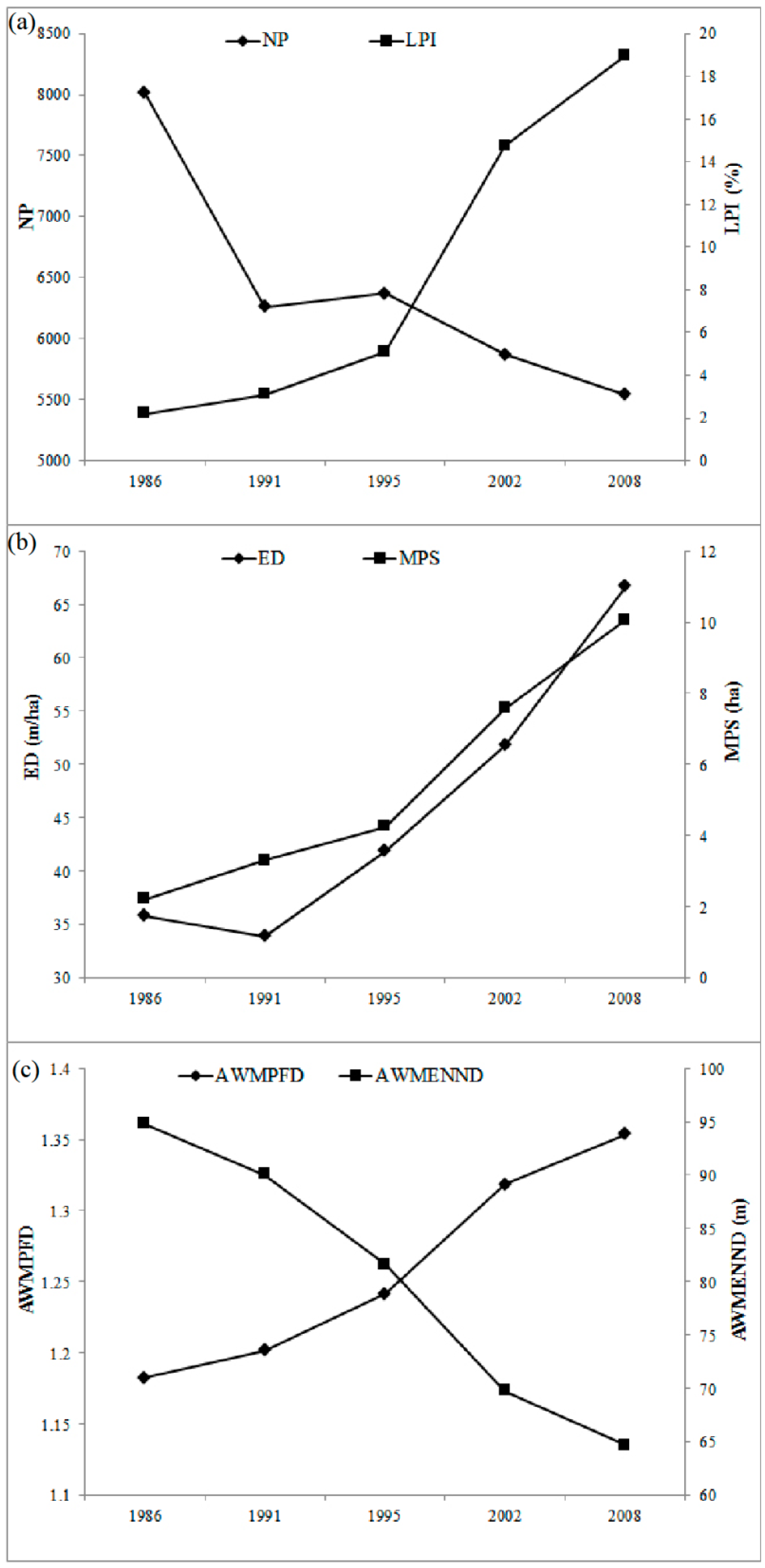
3.1. Changes in Landscape Characteristics

During the period from 1986 to 2008, the urban land increased rapidly and continuously in Suzhou city. In 1986, the built-up area was 168.84 km2 (9.32% of the study area), while, in 2008, the area expanded to 552.47 km2 (30.85% of the study area), representing an increase of 327%. The average annual growth rate also increased greatly, which were 15.99, 26.66, 30.21, and 42.45 km2/year for the four periods of 1986–1991, 1991–1995, 1995–2002, and 2002–2008, respectively, indicating that urbanization in Suzhou had been accelerated over the past 22 years. Most of the new urban land was converted from agricultural land. The accelerated urbanization was accompanied by a massive loss of agricultural land in Suzhou.
The changes in selected landscape metrics are illustrated in Figure 4. NP was 8016 in 1986; it decreased to 6263 in 1991 but increased to 6373 in 1995 and then decreased again to 5869 in 2002 and to 5540 in 2008. LPI continuously increased from 2.21% in 1986 to 18.98% in 2008, indicating that the main urban patch (corresponding to the urban core) became more dominant in the landscape. ED and MPS both had an ascending tendency despite a slight descending of ED in 1991, which indicates that the average length and size of the urban patch type had increased. At the same time, AWMPFD also showed an upward tendency, indicating an increase in the urban patch shape complexity. AWMENND continuously decreased from 95 m in 1986 to 65 m in 2008, which indicates that urban patches became closer to each other. The changes in these landscape metrics suggested that many urban patches might have joined each other as they expanded in the process of urbanization. Therefore, their total number decreased and their average length and size increased.

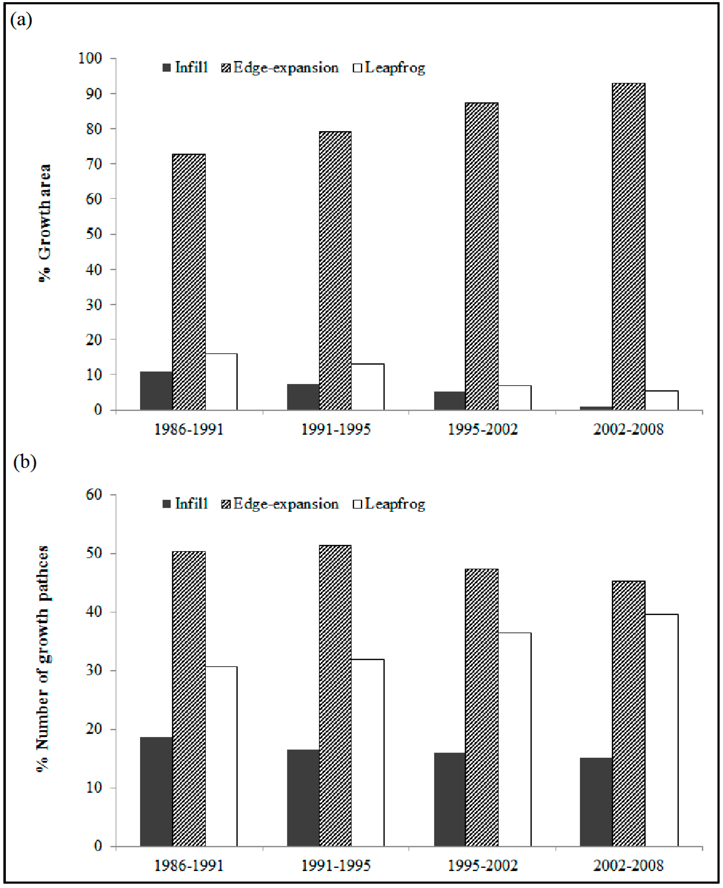
3.2. Typology of Urban Growth

Three urban growth types were identified, and the contribution of each type to the growth area was shown in Figure 5a. Obviously, edge-expansion was the primary growth type throughout the 22-year period. In the first period (1986–1991), the infill growth accounted for 10.86% of total newly developed urban land, while the edge-expansion growth took up 73.07% and the leapfrog type 16.07%. From 1991 to 2002, the percentage of the infill growth decreased to 5.15% and that of the leapfrog growth decreased to 7.14%. In contrast, the edged-expansion type increased to 87.70%. In the last period (2002–2008), the infill growth decreased to a negligible portion of 1% and the leapfrog type to slightly higher than 5%, while the edged-expansion type clearly dominated the new urban area with a percentage of 93.24%.
The NP portion of three growth types exhibited a different trend in the temporal pattern (Figure 5b). The edge-expansion growth had the largest percentage in patch number with a slight decrease from 50.46% in the first period to 45.31% in the last period. The infill type also decreased from 18.70% to 15.03%, whereas the leapfrog growth gradually increased from 30.85% to 39.66%. Throughout the 22 years, edge-expansion always had the largest portion, the leapfrog the second largest, and the infill the smallest one.
During the early stage of urban land expansion in Suzhou, there were gaps between those pre-growth urban patches; the leapfrog growth urban patches were isolated from the dominant urban core. As the urbanization process proceeded in Suzhou, those gaps were gradually filled by infilling growth patches, which also connected some of the pre-growth urban patches. At the same time, with the continuous edge-expansion the urban core expanded outwards and gradually approached and eventually joined those formerly isolated leapfrog urban patches.

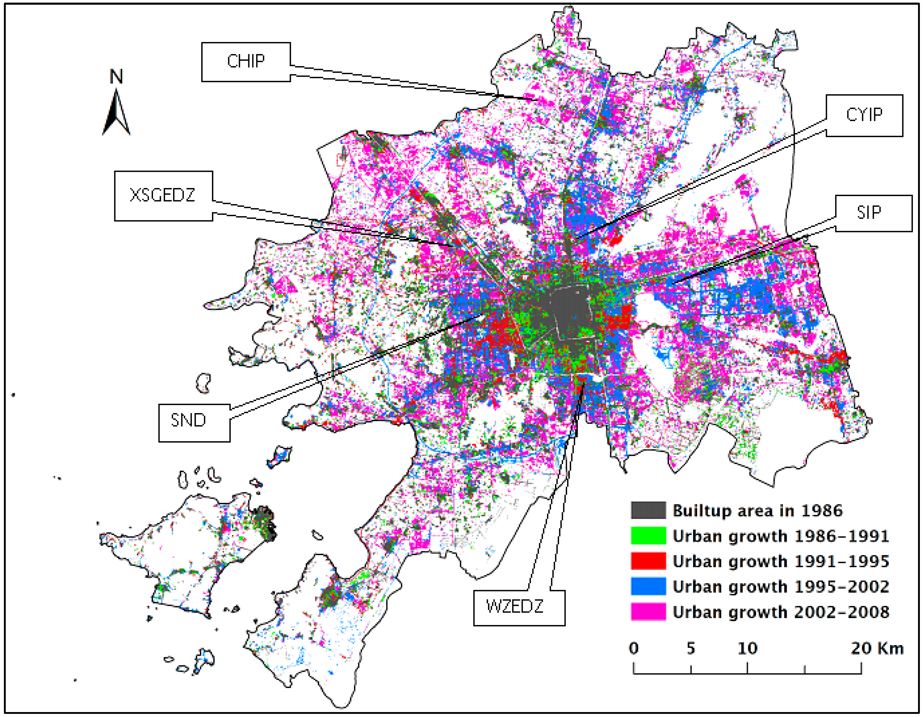
3.3. Changing Urban Growth Patterns

Based on results from land use classification (Figure 6), sector analysis (Figure 7), and concentric circle analysis (Figure 8), we can analyze the changing urban growth patterns during different periods in detail. During the first period (1986–1991), urban land increased almost at the same rate along the 16 directional axes; urban growth concentrated around the pre-growth urban core (the old city district); and a few new built-up patches developed at some towns and townships away from the city center. The curve depicting the percentage of new urban area by distance to the city center had multiple peaks, which reflected hot-zones of urban growth in this period (Figure 8). The first peak occurred at the distance of 4–6 km with the single largest percentage of growth area. This corresponded to the new urban land developed around the urban core. At the distance of 10–20 km, there was the largest concentration (almost half) of growth area, which reflected the new built-up area in those towns and townships.
From 1991 to 1995, the urban growth rate showed great variation along different directions. The highest growth rates took place along the E, SWW, NWW, and NW directions (Figure 7). Figure 6 also clearly reflects this pattern. The development of the China–Singapore Suzhou Industrial Park (SIP) to the east of the old city district and the Suzhou New and High-Tech District (SND) to the west significantly expanded the urban core. The first peak with the largest percentage of growth area, which represented the urban fringe, moved outward to the distance of 6–8 km (Figure 8).
During the third period (1995–2002), the highest growth rates occurred along the N, NNE, E, SWW, SSE, and NNW directions (Figure 7). This reflected the rapid expansion of SIP, Wuzhong Economic Development Zone (WZEDZ), SND, and Xushuguan Economic Development Zone (XSGEDZ). Urban growth was obviously development zone oriented in this period. The construction of transportation infrastructure (highways and local arterial roads), which aimed to improve the accessibility of adjacent development zones, was clearly reflected in Figure 6. The urban fringe further moved to the distance of 8–10 km (Figure 8).
From 2002 to 2008, the largest newly developed urban areas took place along the NEE and NW directions, which were closely related to the further development of SIP and the establishment of Chengyang Industrial Park (CYIP) and Caohu Industrial Park (CHIP). The urban fringe had moved to the distance of 10–12 km by 2008 (Figure 8). Percentages of new urban area at the zones within the distance of 10 km from the city center were much lower than those of previous period. Urban growth mostly occurred at the distance of 12–24 km, within which the percentages of growth area were the highest among the four periods. Compared with the previous three periods, urban expansion took place at more distant locations, especially at the concentric zones of 20–24 km distance. We noticed that built-up area decreased along the SWW and W directions during this period. This was partially the result of restoration of inefficiently used or abandoned industrial (manufacturing and mining) and rural residential land in this area [39].

3.4. Economic Transition and Urban Growth

Changing urban growth patterns from 1986 to 2008 in Suzhou were actually the result of economic transition in the past three decades. Urban growth changed from bottom-up rural urbanization to top-down urban expansion during the 22 years. The underlying mechanism for urbanization changed from TVEs-driven rural industrialization to FDI-driven development zone fever.

3.4.1. From Bottom-Up Rural Urbanization to Top-Down Urban Expansion

Suzhou is located in the heart of the Sunan region, where the orthodox Sunan model attributed the early development (from 1978 to the early 1990s) of Sunan to the local state-directed TVEs [21]. During this period, economic growth and urbanization mainly took place in the rural areas. Rural-dominated urbanization dispersed all over the countryside of Sunan region because rural industry was widely dispersed in small towns and villages [40]. Such a trajectory of urbanization based on the growth of towns and townships is called ‘urbanization from below’, which is quite different from the city-based urbanization track, which is often called ‘urbanization from above’ [41,42]. This bottom-up rural urbanization was characteristic of unplanned spontaneous growth of town and town economy without significant investment from the central government [42]. This type of urbanization was slight and stable due to the small-scale of most TVEs. Therefore, from 1986 to 1991, urban land increased modestly in Suzhou and almost half of the growth area took place in those towns and townships away from the city center.
Since the early-1990s, the combined effect of the influx of FDI and government support to urban economies has created a more competitive market in which TVEs gradually lost their advantages. Suzhou gradually moved beyond the traditional Sunan Model through globalization and emerged as a hot manufacturing center and a major FDI destination in China [20,21]. This top-down urban expansion created a rising demand for industrial land, which was mostly satisfied by converting agricultural land. The establishment of SND in 1992 and SIP in 1994 manifested the significant investment from above (the central government) and from outside (Singapore), which also modified the urbanization process from rural-dominated to city-based.

3.4.2. From TVE-Driven Urbanization to FDI-Driven Development Zone Fever

The bottom-up rural urbanization was mainly driven by TVEs. From 1978 to the early 1990s, TVEs dominated the economic and industrial structure of Suzhou. The widely dispersed rural industry could absorb rural surplus labors into TVEs, which allowed people to leave the field without leaving the village (litu bu lixiang). However, TVEs began to experience a slowdown in the early 1990s because of unclear property rights and inefficient management. While TVEs underwent restructuring and privatization, a large amount of foreign investment was infused into Suzhou shortly after the development of the Pudong New Area in Shanghai in 1992. The 2000s witnessed an unprecedented increase of FDI in Suzhou (Figure 9). Many of the Fortune Global 500 Companies, such as Siemens, Samsung, Fujitsu, and Philips, have invested in Suzhou.
Since the mid-1990s, urban land expansion in Suzhou has been mainly stimulated by FDI-driven industrialization. Foreign investment oriented development zones expanded rapidly and accounted for a large portion of the new urban area. In addition to major national and provincial development zones, some town-level governments also entered the race for foreign investment by setting up their own development zones (so-called ‘one town, one zone’). In order to attract FDI to stimulate the local economy, almost every town planned its own industrial estate and preferential policies, one of which was low-cost land use. As a result, a development zone fever emerged in the late 1990s [14,43,44,45].
This tide of zone development without any rational plan swept coastal China and caused a dramatic urban land expansion. A lack of scientific plans for industrial development resulted in the insufficient use of development zones and a waste of valuable agricultural land. In the summer of 2003, the central government released two decrees, stopped approving any new development zones, and urged local governments to clean up the existing zones [11]. As a result, many unofficially approved development zones were revoked and restored to agricultural use. This might partially explain the decrease of built-up area along the SWW and W directions from 2002 to 2008.
From 1986 to 2008, rapid urban expansion resulted in many environmental problems and posed challenges for environmental sustainability in Suzhou. Massive agricultural land loss has changed Suzhou from a traditional rice production base to an area that heavily relies on imported rice and has raised concern for food security [46]. Unprecedented urbanization and industrialization has caused eutrophication and algal bloom in Taihu Lake and greatly impacted the quality and quantity of water supplies in the Taihu Basin [47]. Land use regulation from the local government was not effective in curbing the urban sprawl during this period. For the sustainable development of Suzhou, government intervention and strict land use policies are highly needed in this rapidly urbanizing city. Sustainable development strategies such as smart growth and compact development should be advocated in Suzhou [48].

4. Spatial Determinants of Urban Growth

4.1. Global Logistic Regression Model

As analyzed in the previous section, an economic transition in Suzhou took place in the early 1990s. In addition, the administrative division and transportation network were mostly formed in the 1990s. Therefore, we chose the year 1991 as the starting year for the land conversion model. The results of the global logistic regression model are presented in Table 4. The percentage correctly predicted is 76.6%, which indicates moderate prediction accuracy. The independent variables are all significant; Dis2Indu at the 0.1 level and all the other variables at the 0.01 level.
Among the three proximity variables, distance to local arterial roads (Dis2Lard) had the strongest negative effect on land conversion, and distance to railways (Dis2Rail) had the second strongest. Contrary to our expectations, distance to highways (Dis2Hwy) had a minor positive effect. The significance of local arterial roads in land use conversion is similar to the findings of previous studies [7,8]. The findings suggest that urban growth in Suzhou was largely dependent on transportation infrastructure development and that local roads were a more important determinant.
The two variables representing neighborhood physical conditions, density of waters (DenWater) and slope (Slope), both had a negative effect on urban land conversion. This indicates that urban expansion is generally constrained by water density and topographical condition. Density of waters (DenWater) actually had the strongest negative effect among all variables. This was probably because major water bodies and wetlands were protected in Suzhou. Among the socioeconomic variables, only the distance to district center (DisDcen) had a negative coefficient, which indicates that as the distance to a district center increased, the probability for a pixel to convert from nonurban to urban land decreased. Distance to industrial centers (Dis2Indu) had a positive effect on urban growth, which might indicate that urban development was not dependent on the existing industrial centers in Suzhou. Density of built-up area (DenBuilt) in the neighborhood had the strongest positive effect among all variables. It played a significant promotional role for urban land conversion.
Our global logistic regression model can explain the determinants of urban land conversion in Suzhou. However, the potential spatial non-stationarity of urban growth is still unknown. We further use logistic GWR for the detection of spatial non-stationarity, as it allows the regression parameters to vary across space and can therefore expose local spatial variations of urban growth patterns in Suzhou.

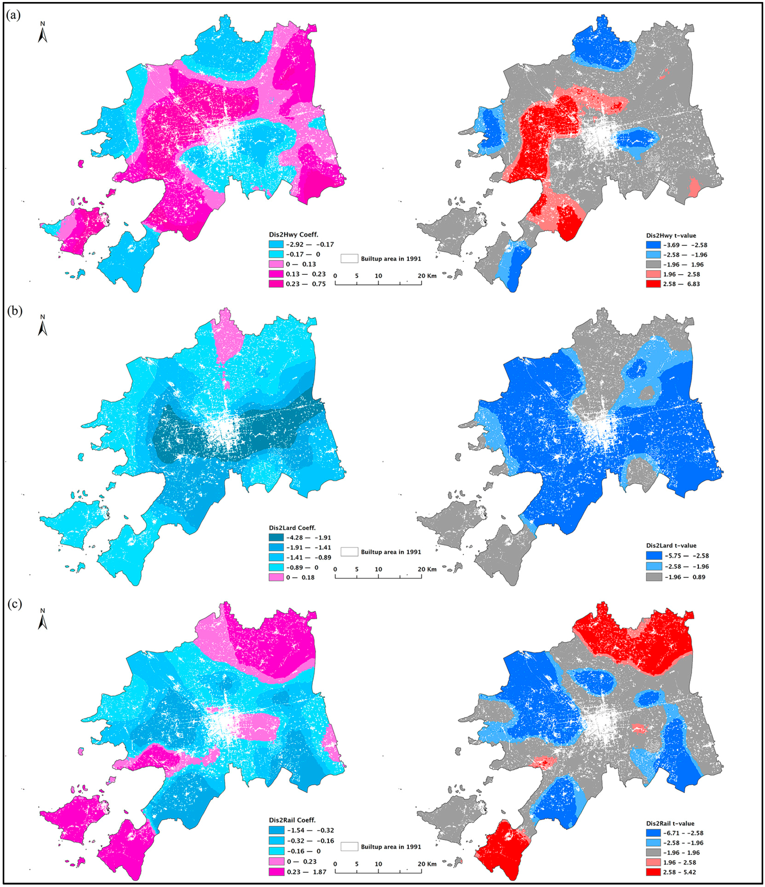
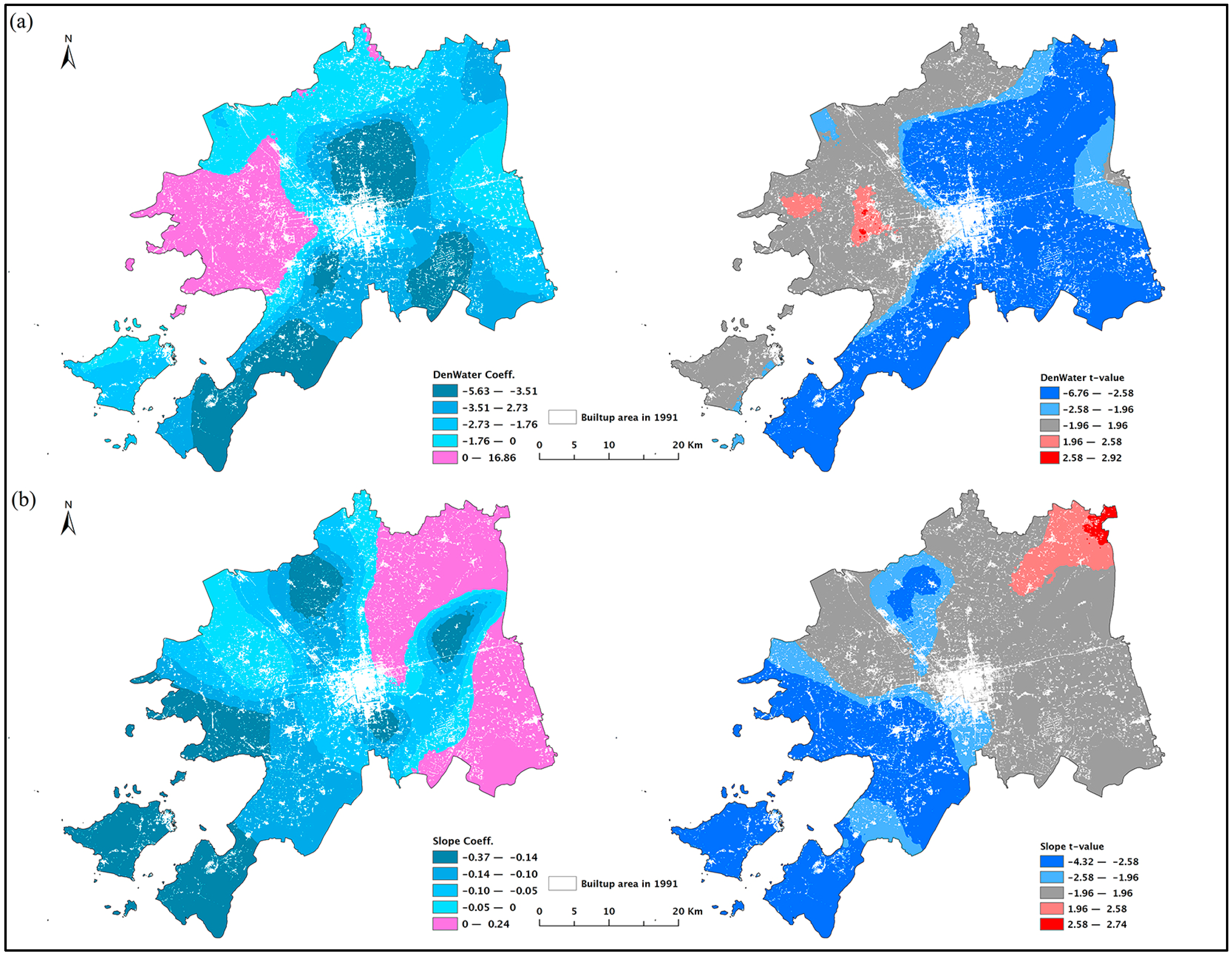
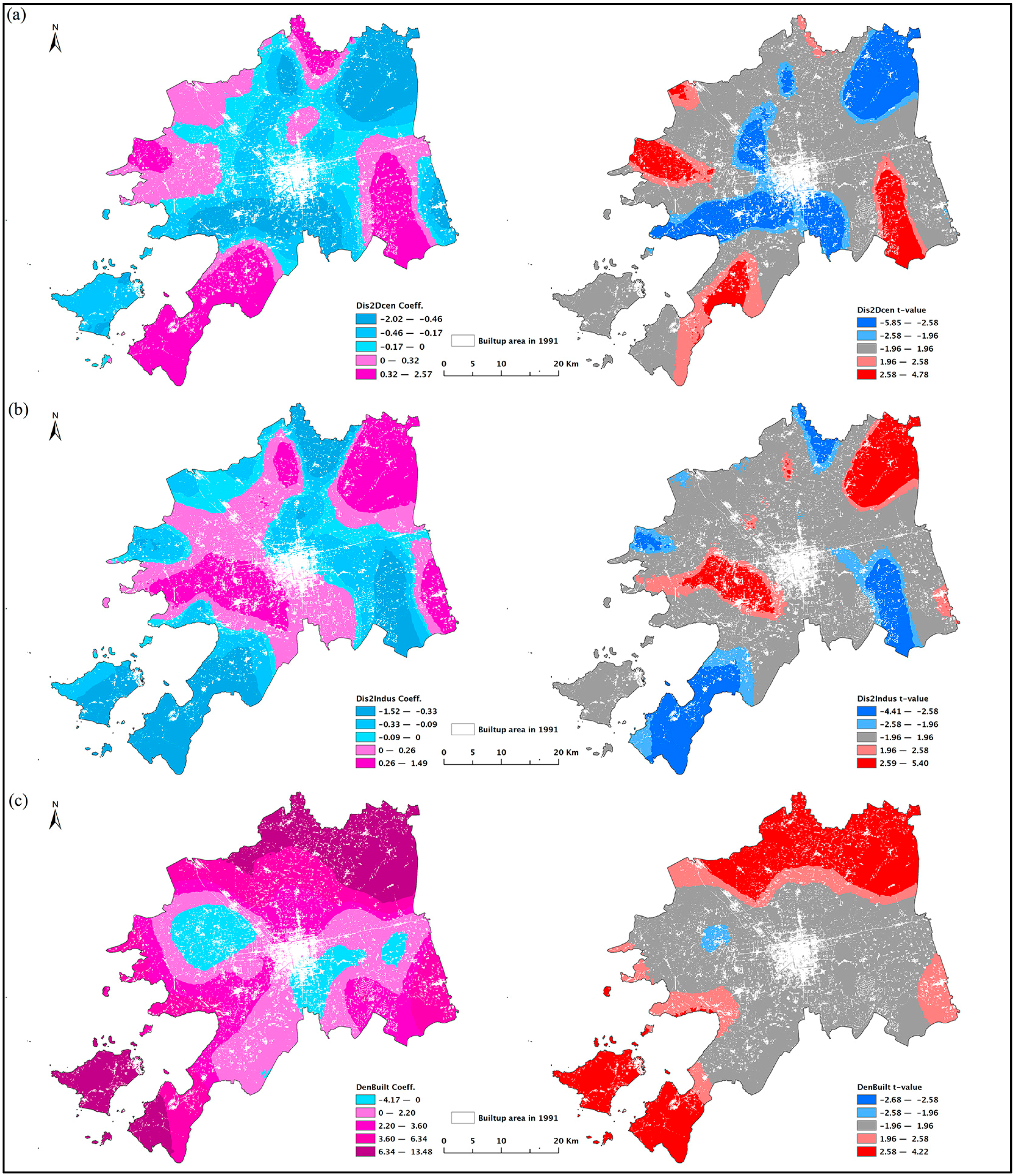
4.2. Spatial Variations of Urban Growth Patterns

We applied the geographically weighted logistic regression to the same dataset of 4818 sample points. Table 5 represents a comparison between the global logistic model and the logistic GWR model. The logistic GWR model shows a clear improvement over the global logistic model. First, the decreases in -2 Log-Likelihood, residual sum of squares, and AICc and the increase of Pseudo R squared indicate that the GWR model has a much better goodness-of-fit than the global model. Second, the increases of PCP and ROC (area under the receiver operating characteristic curve) suggest that the logistic GWR model has higher prediction accuracy. Third, the GWR model has remarkably reduced the spatial dependence of residuals, which can be measured by the decrease in Moran’s I of residuals.
Different from the global logistic model, the values of parameter estimates of the logistic GWR model show significant variations. Table 6 represents the summary statistics of the GWR parameter estimates for the sample points. All the variables have both positive and negative parameter values, although they have variations in the portions of both values. The parameter values of Dis2Hwy, Dis2Rail, slope, Dis2Dcen, and Dis2Indu have a clear division of positive and negative results. Such significant spatial variations are ignored by the global logistic model but can be detected by the GWR model. The parameter values of Dis2Lard, DenWater, and DenBuilt have relatively low levels division of positive and negative results, which indicates that these variables have fewer spatial variations.
The software package GWR4 generated a set of parameter estimates for each sample point. In addition, pseudo t-statistics was also calculated to indicate the significance of the parameters. Based on the sample points with parameter estimates and t-statistics, a set of parameter and t-statistics surfaces were generated to reveal the spatial variation of urban land growth patterns. An inverse distance weighted (IDW) interpolation was employed to generate these surfaces. The IDW interpolation method assumes that the surface is driven by the local variations, which can be captured through the neighborhood [8]. Figure 10, Figure 11 and Figure 12 represent the generated parameter and t-statistics surfaces with a cell size of 30 m × 30 m. Different from the global logistic model in which the parameters are unified across space, it is clear from Figure 10, Figure 11 and Figure 12 that all parameters vary across the study area. In terms of significance, all the parameters have certain parts in the study area where they are not statistically significant.
Figure 10 presents the parameter and t-statistic surfaces of the three variables of proximity to transportation networks. While the global logistic regression model indicated that the distance to highways (Dis2Hwy) had positive influence on urban land development, the parameter surface of Dis2Hwy suggests that there were portions in the northwestern, northern, central, southeastern, and southwestern regions of the study area where the distance to highways had negative effect on urban land conversion (Figure 10a). Negative coefficients of Dis2Hwy were significant in the north of the city (Caohu Industrial Park), to the east of the pre-growth urban core (Suzhou Industrial Park), in the south of the Dongshan Peninsula, and around the shoreline of Taihu Lake in the west of the city. This may indicate that the development of Suzhou Industrial Park (SIP) and Caohu Industrial Park (CHIP) depended more on intercity highways than other areas. SIP and CHIP are both export-oriented development zones, which imply that transportation planning should reinforce the importance of highways for export-oriented areas in the future. The distance to local arterial roads (Dis2Lard) had a dominantly negative influence on land conversion, except in a very small area in the north of the city (Figure 10b). This influence was strongest next to the original urban core along an east-west axis and decreased towards south and north. The parameter of Dis2Lard was significant for most of the study area, except to the north of the pre-growth urban core and on the two islands where local roads mostly encircled mountains (Figure 3). The global logistic regression model showed that the distance to railways (Dis2Rail) had a negative influence on urban land expansion. However, this was not true for the whole study area. The positive influence of Dis2Rail could be found in the northeastern part, east of the original urban core (Suzhou Industrial Park), and in the two islands, but the positive influence was significant only in the northeast and on the Dongshan Peninsula (Figure 10c).
The logistic GWR model also revealed the spatial variation of the parameter estimates of the two variables for neighborhood physical conditions. The density of waters (DenWater) largely had a negative influence on land conversion, except in the western part (Figure 11a). The western part of Suzhou does not have many large water bodies (Figure 3), such as lakes and rivers, which are often protected. The parameter of DenWater was significant in most areas in the northeastern, eastern, southern, and southwestern regions of the study area. Representing the topographical conditions, slope generally exerted a negative impact on urban growth in Suzhou (Figure 11b). However, slope did have a positive influence in the northeastern and southeastern parts of the city, where two large inland lakes, Yangcheng Lake and Cheng Lake, are located. The coefficients of slope were negatively significant in the southwestern part of the study area and positively significant only in the northeastern corner. The spatial distribution of slope in Suzhou confirms that the southwestern part has low mountains where the steep topography would adversely impact urban growth (Figure 3).
Figure 12 presents the parameter and t-statistic surfaces of the three socioeconomic variables. Although the distance to district center (Dis2Dcen) had a weaker negative influence in the global model, its parameter surface varied greatly across the space (Figure 12a). This variable had a positive effect on urban land development in the northern, southeastern, southwestern, and northwestern parts of the city. The coefficients of Dis2Dcen were negatively significant in the northeastern (Yangcheng Lake) and southern (Wuzhong Economic Development Zone) regions of the study area and west and northwest of the original urban core (SND and Xushuguan Development Zone) and were positively significant only in a small portion of the southeastern, southwestern, and northwestern part of the study area. The global model demonstrated that urban development was not dependent on existing industrial centers. Logistic GWR found that this statement was oversimplified. Although the distance to industrial centers (Dis2Indu) had a positive influence to the south, west, and northwest of the pre-growth urban center and the northeastern part of the city, the parameter of Dis2Indu was positively significant only to the west of the original urban core and in the northeastern part of the study area (Figure 12b). Coefficients of this variable were negatively significant only in a small portion of the southeastern part and in the southwestern part of the city. For the majority of the city, the parameter Dis2Indu was not statistically significant. Similarly, the density of built-up area (DenBuilt) had a dominantly positive influence on land conversion (Figure 12c), but its parameter was not statistically significant in most parts of the city. Only in the north of the city and in the two islands were the coefficients of DenBuilt positively significant. These areas were less urbanized in the pre-growth period, and this may indicate that existing built-up area could play a more effective role in promoting urban growth in less mature areas.

5. Conclusions

This paper analyzes the spatiotemporal dynamics of urban growth and models its spatial determinants in urban China through a case study of Suzhou. We have contributed to the research on urban development in Chinese cities by investigating the unique transition from bottom-up rural urbanization to top-down urban expansion in Suzhou. We used landscape metrics, spatial analysis, and GIS to analyze land use data derived from remote sensing images and developed global and local logistic regression models, which integrated a set of spatial variables to analyze the patterns and underlying factors of urban growth in Suzhou. We found that, from 1986 to 2008, the built-up areas in Suzhou had increased from 9.32% to 30.85% of the study area and the average annual growth rate had accelerated.
Landscape metrics and spatial analysis have quantified the spatiotemporal dynamics of urban development in Suzhou. We distinguished three types of urban growth, of which edge-expansion growth dominated the new urban area, while infilling and leapfrog growth decreased over the study period. Sector and concentric circle analyses have identified the changing directions and hot-zones of urban growth in Suzhou, which mostly overlapped with the FDI-driven development zones. Rapid urban growth has caused serious environmental problems. Effective land use regulation and sustainable development strategies should be advocated [49].
In our global logistic regression model, all of the independent variables were statistically significant. Among the proximity variables, distance to the local arterial roads had the strongest negative influence on land conversion. Density of waters as well as slope in the neighborhood also had negative effects. Among the socioeconomic variables, the density of built-up area tended to promote urban growth, while increased distance to the district center would decrease the probability of land conversion.
We found that the logistic GWR model improved over the global logistic regression model. Logistic GWR had a better overall goodness-of-fit and higher prediction accuracy than the global model. Therefore, it had better performance in exploring the relationships between the underlying factors and urban growth patterns. In addition, logistic GWR remarkably reduced the spatial dependence of residuals measured by the decrease in Moran’s I of residuals.
In addition, the logistic GWR model allowed the parameters to vary across space, which provided more insights into the spatial variations of urban growth patterns. Each variable had both negative and positive influence on urban growth in different parts of the study area. The distance to local arterial roads and the density of waters had a predominantly negative influence, and their coefficients were significant in most parts of the city. The other variables tended to have very local influence and their coefficients were statistically significant only in a very small area. Although logistic GWR could more effectively reveal spatial variations in the influence of independent variables, the interpretation of these variations should be closely related to the specific context of the study area.

Acknowledgments

The authors would like to acknowledge the funding of the Ford Foundation (0155-0883) and the National Natural Science Foundation of China (41329001, 41130750).

Author Contributions

Ling Zhang collected and prepared the data. Ling Zhang and Ran Meng analyzed the data. Ling Zhang and Yehua Dennis Wei contributed to the conceptual framework and research design and wrote the paper.

Conflicts of Interest

The authors declare no conflict of interest.

References

  1. Yeh, A.G.O.; Li, X. Economic development and agricultural land loss in the Pearl River Delta, China. Habitat Int. 1999, 23, 373–390. [Google Scholar]
  2. Seto, K.C.; Woodcock, C.E.; Song, C.; Huang, X.; Lu, J.; Kaufmann, P.K. Monitoring land-use change in the Pearl River Delta using Landsat TM. Int. J. Remote Sens. 2002, 23, 1985–2004. [Google Scholar] [CrossRef]
  3. Long, H.L.; Tang, G.P.; Li, X.B.; Heilig, G.K. Socio-economic driving forces of land use change in Kunshan, the Yangtze River Delta economic area of China. J. Environ. Manag. 2007, 83, 351–364. [Google Scholar] [CrossRef] [PubMed]
  4. Page, J.; Davis, B.; Areddy, J. China turns predominantly urban. The Wall Street Journal, 18 January 2012; A10. [Google Scholar]
  5. Xie, Y.C.; Yu, M.; Bai, Y.F.; Xing, X.R. Ecological analysis of an emerging urban landscape pattern—Desakota: A case study in Suzhou, China. Landsc. Ecol. 2006, 21, 1297–1309. [Google Scholar] [CrossRef]
  6. Wei, Y.H.D. Regional development in China: Transitional institutions, embedded globalization, and hybrid economies. Eurasian Geogr. Econ. 2007, 48, 16–36. [Google Scholar] [CrossRef]
  7. Cheng, J.Q.; Masser, I. Urban growth pattern modeling: A case study of Wuhan city, PR China. Landsc. Urban Plan. 2003, 62, 199–217. [Google Scholar] [CrossRef]
  8. Luo, J.; Wei, Y.H.D. Modeling spatial variations of urban growth patterns in Chinese cities: The case of Nanjing. Landsc. Urban Plan. 2009, 91, 51–64. [Google Scholar] [CrossRef]
  9. Liao, F.H.F.; Wei, Y.H.D. Modeling determinants of urban growth in Dongguan, China: A spatial logistic approach. Stoch. Environ. Res. Risk Assess. 2014, 28, 801–816. [Google Scholar] [CrossRef]
  10. Lin, G.C.S.; Wei, Y.H.D. China’s restless urban landscape 1: New challenge for theoretical reconstruction. Environ. Plan. A 2002, 34, 1535–1544. [Google Scholar] [CrossRef]
  11. Deng, F.F.; Huang, Y.Q. Uneven land reform and urban sprawl in China: The case of Beijing. Prog. Plan. 2003, 61, 211–236. [Google Scholar] [CrossRef]
  12. Lin, G.C.S.; Ho, S.P.S. The state, land system, and land development processes in contemporary China. Ann. Assoc. Am. Geogr. 2005, 95, 411–436. [Google Scholar] [CrossRef]
  13. Wei, Y.H.D. Restructuring for growth in urban China: Transitional institutions, urban development, and spatial transformation. Habitat Int. 2012, 36, 396–405. [Google Scholar] [CrossRef]
  14. Wei, Y.H.D. Zone fever, project fever: Development policy, economic transition, and urban expansion in China. Geogr. Rev. 2015, 105, 156–177. [Google Scholar] [CrossRef]
  15. Xie, Y.C.; Batty, M.; Zhao, K. Simulating emergent urban form using agent-based modeling: Desakota in the. Suzhou-Wuxian region in China. Ann. Assoc. Am. Geogr. 2007, 97, 477–495. [Google Scholar] [CrossRef]
  16. Li, X.; Yeh, A.G.O. Modelling sustainable urban development by the integration of constrained cellular automata and GIS. Int. J. Geogr. Inf. Sci. 2000, 14, 131–152. [Google Scholar] [CrossRef]
  17. Li, X.; Yeh, A.G.O. Neural-network-based cellular automata for simulating multiple land use changes using GIS. Int. J. Geogr. Inf. Sci. 2002, 16, 323–343. [Google Scholar] [CrossRef]
  18. McDonald, R.I.; Urban, D.L. Spatially varying rules of landscape change: Lessons from a case study. Landsc. Urban Plan. 2006, 74, 7–20. [Google Scholar] [CrossRef]
  19. Luo, J.; Yu, D.L.; Xin, M. Modeling urban growth using GIS and remote sensing. GISci. Remote Sens. 2008, 45, 426–442. [Google Scholar] [CrossRef]
  20. Wei, Y.H.D.; Lu, Y.Q.; Chen, W. Globalizing regional development in Sunan, China: Does Suzhou Industrial Park fit a Neo-Marshallian District model? Reg. Stud. 2009, 43, 409–427. [Google Scholar]
  21. Wei, Y.H.D. Beyond the Sunan model: Trajectory and underlying factors of development in Kunshan, China. Environ. Plan. A 2002, 34, 1725–1747. [Google Scholar]
  22. Breiman, L. Random forests. Mach. Learn. 2001, 45, 5–32. [Google Scholar] [CrossRef]
  23. Liaw, A.; Wiener, M. Classification and regression by random forest. R News 2002, 2, 18–22. [Google Scholar]
  24. Liu, Y.; Yue, W.Z.; Fan, P.L. Spatial determinants of urban land conversion in large Chinese cities: A case of Hangzhou. Environ. Plan. B 2011, 38, 706–725. [Google Scholar] [CrossRef]
  25. Herold, M.; Scepan, J.; Clarke, K.C. The use of remote sensing and landscape metrics to describe structures and changes in urban land uses. Environ. Plan. A 2002, 34, 1443–1458. [Google Scholar] [CrossRef]
  26. Seto, K.C.; Fragkias, M. Quantifying spatiotemporal patterns of urban land-use change in four cities of China with time series landscape metrics. Landsc. Ecol. 2005, 20, 871–888. [Google Scholar] [CrossRef]
  27. McGarigal, K.; Cushman, S.A.; Neel, M.; Ene, E. FRAGSTATS Version 4: Spatial Pattern Analysis Program for Categorical Maps; University of Massachusetts: Amherst, MA, USA, 2002; Available online: http://www.umass.edu/landeco/research/fragstats/fragstats.html (accessed on 6 March 2017).
  28. Yue, W.Z.; Liu, Y.; Fan, P.L. Polycentric urban development: The case of Hangzhou. Environ. Plan. A 2010, 42, 563–577. [Google Scholar] [CrossRef]
  29. Luck, M.; Wu, J. A gradient analysis of urban landscape pattern: A case study from the Phoenix metropolitan region, Arizona, USA. Landsc. Ecol. 2002, 17, 327–339. [Google Scholar] [CrossRef]
  30. Xu, C.; Liu, M.; Zhang, C.; An, S.Q.; Yu, W.; Chen, J.M. The spatiotemporal dynamics of rapid urban growth in the Nanjing metropolitan region of China. Landsc. Ecol. 2007, 22, 925–937. [Google Scholar] [CrossRef]
  31. Xu, J.G.; Liao, B.G.; Shen, Q.; Zhang, F.; Mei, A.X. Urban spatial restructuring in transitional economy—Changing land use pattern in Shanghai. Chin. Geogr. Sci. 2007, 17, 19–27. [Google Scholar] [CrossRef]
  32. Wu, F.L.; Yeh, A.G.O. Changing spatial distribution and determinants of land development in Chinese cities in the transition from a centrally planned economy to a socialist market economy: A case study of Guangzhou. Urban Stud. 1997, 34, 1851–1879. [Google Scholar] [CrossRef]
  33. Verburg, P.H.; van Eck, J.R.R.; de Nijs, T.C.M.; Dijst, M.J.; Schot, P. Determinants of land-use change patterns in the Netherlands. Environ. Plan. B 2004, 31, 125–150. [Google Scholar] [CrossRef]
  34. Seto, K.C.; Kaufmann, R.K. Modeling the drivers of urban land use change in the Pearl River Delta, China: Integrating remote sensing with socioeconomic data. Land Econ. 2003, 79, 106–121. [Google Scholar] [CrossRef]
  35. Fotheringham, A.S.; Brunsdon, C.; Charlton, M.E. Geographically Weighted Regression: The Analysis of Spatially Varying Relationships; John Wiley & Sons Ltd.: Chichester, UK, 2002. [Google Scholar]
  36. Fotheringham, A.S.; Charlton, M.E.; Brunsdon, C. Spatial variations in school performance: A local analysis using geographically weighted regression. Geogr. Environ. Model. 2001, 5, 43–66. [Google Scholar] [CrossRef]
  37. Gilbert, A.; Chakraborty, J. Using geographically weighted regression for environmental justice analysis: Cumulative cancer risks from air toxics in Florida. Soc. Sci. Res. 2011, 40, 273–286. [Google Scholar] [CrossRef]
  38. Nakaya, T. GWR4 User Manual. GWR 4 Development Team, 2014. Available online: https://geodacenter.asu.edu/drupal_files/gwr/GWR4manual.pdf (accessed on 12 December 2015).
  39. Chen, X.Y. Land restoration resulted in 55 thousand mu of new agricultural land during the past 8 years in Suzhou. Suzhou Daily, 2014; 30, A1. [Google Scholar]
  40. Ho, S.P.S.; Lin, G.C.S. Non-Agricultural land use in post-reform China. China Q. 2004, 179, 758–781. [Google Scholar] [CrossRef]
  41. Cui, G.H.; Ma, L.J.C. Urbanization from below in China: Its development and mechanism. Acta Geogr. Sin. 1999, 54, 106–115. (In Chinese) [Google Scholar]
  42. Ma, L.J.C.; Fan, M. Urbanization from below: The growth of towns in Jiangsu, China. Urban Stud. 1994, 31, 1625–1645. [Google Scholar] [CrossRef]
  43. Cartier, C. ‘Zone fever’, the arable land debate, and real estate speculation: China’s evolving land use regime and its geographical contradictions. J. Contemp. China 2000, 10, 445–469. [Google Scholar] [CrossRef]
  44. Yang, D.Y.R.; Wang, H.K. Dilemmas of local governance under the development zone fever in China. Urban Stud. 2008, 45, 1037–1054. [Google Scholar] [CrossRef]
  45. Gao, J.; Wei, Y.D.; Chen, W.; Yenneti, K. Urban land expansion and structural change in the Yangtze River Delta, China. Sustainability 2015, 7, 10281–10307. [Google Scholar] [CrossRef]
  46. Qin, B.Q.; Xu, P.Z.; Wu, Q.L.; Luo, L.C.; Zhang, Y.L. Environmental issues of Lake Taihu, China. Hydrobiologia 2007, 581, 3–14. [Google Scholar] [CrossRef]
  47. Li, G.L.; Chen, J.; Sun, Z.Y. Non-agricultural land expansion and its driving forces: A multi-temporal study of Suzhou, China. Int. J. Sustain. Dev. World Ecol. 2007, 14, 408–420. [Google Scholar] [CrossRef]
  48. Dahal, K.R.; Benner, S.; Lindquist, E. Urban hypotheses and spatiotemporal characterization of urban growth in the Treasure Valley of Idaho, USA. Appl. Geogr. 2017, 79, 11–25. [Google Scholar] [CrossRef]
  49. Wei, Y.H.D. Towards equitable and sustainable urban space. Sustainability 2016, 8, 804. [Google Scholar] [CrossRef]
Figure 1. Location and administrative division of Suzhou City, 2008.
Sustainability 09 00393 g001
Figure 2. (a) Sector and (b) concentric circle analyses.
Sustainability 09 00393 g002
Figure 3. Spatial distribution of (a) roads, railways, and centers; (b) slope; (c) water and wetland in Suzhou city.
Sustainability 09 00393 g003
Figure 4. Changes in the landscape metrics during the period of 1986–2008: (a) number of patches (NP) and largest patch index (LPI); (b) edge density (ED) and mean patch size (MPS); (c) area-weighted mean patch fractal dimension (AWMPFD); and (d) area-weighted mean Euclidean nearest-neighbor distance (AWMENND).
Sustainability 09 00393 g004
Figure 5. The proportion of (a) growth area and (b) patch number of the three urban land growth types in different periods.
Sustainability 09 00393 g005
Figure 6. Major development zones and urban growth in Suzhou City, 1986–2008. Caohu Industrial Park (CHIP), Chengyang Industrial Park (CYIP), Suzhou Industrial Park (SIP), Xushuguan Economic Development Zone (XSGEDZ), Suzhou New and High-Tech District (SND), and Wuzhong Economic Development Zone (WZEDZ).
Sustainability 09 00393 g006
Figure 7. Spatial orientation of urban land expansion in Suzhou, 1986–2008.
Sustainability 09 00393 g007
Figure 8. Percentage of new urban area by distance to city center, 1986–2008.
Sustainability 09 00393 g008
Figure 9. Actualized foreign direct investment (FDI) in Suzhou City, 1990–2008.
Sustainability 09 00393 g009
Figure 10. Geographically weighted regression (GWR) coefficient and t-value surfaces of (a) distance to highways; (b) distance to local arterial roads; and (c) distance to railways.
Sustainability 09 00393 g010
Figure 11. GWR coefficient and t-value surfaces of (a) density of waters and (b) slope.
Sustainability 09 00393 g011
Figure 12. GWR coefficient and t-value surfaces of (a) distance to district center; (b) distance to industrial centers; and (c) density of built-up area.
Sustainability 09 00393 g012
Table 1. Selected landscape metrics.
MetricsUnitRangeFormula and Description
NPNoneNP ≥ 0 Sustainability 09 00393 i001
NP equals the number of patches of the corresponding patch type (class)
LPIPercent0 < LPI ≤ 100 Sustainability 09 00393 i002
LPI equals the area (m2) of the largest patch of the corresponding patch type, divided by total landscape area (m2), multiplied by 100 (to convert to a percentage)
EDMeters per hectareED ≥ 0 Sustainability 09 00393 i003
ED equals the sum of the lengths (m) of all edge segments involving the corresponding patch type, divided by the total landscape area (m2), multiplied by 10,000 (to convert to hectares)
MPSHectaresMPS > 0 Sustainability 09 00393 i004
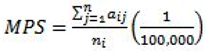
MPS equals the sum of areas (m2) of all patches of the corresponding patch type, divided by the number of patches of the same type, divided by 10,000 (to convert to hectares)
AWMPFDNone1 < AWMPFD ≤ 2 Sustainability 09 00393 i005
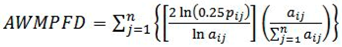
AWMPFD equals the sum, across all patches of the corresponding patch type, of two times the logarithm of 0.25 the times patch perimeter (m), divided by the logarithm of patch area (m2), multiplied by the patch area (m2) divided by total class area
AWMENNDMetersAWMENND ≥ 0 Sustainability 09 00393 i006
AWMENND equals the sum, across all patches of the corresponding patch type, of the nearest neighbor distance of each patch, multiplied by the proportional abundance of the patch (i.e. patch area divided by the sum of patch areas)
NP: number of patches; LPI: largest patch index; ED: edge density; MPS: mean patch size; AWMPFD: area-weighted mean patch fractal dimension; AWMENND: area-weighted mean Euclidean nearest-neighbor distance. Source: McGarigal et al. [27].
Table 2. Variables used in the urban land use conversion models.
VariablesDescriptions
Dependent Variable
 ChangeLand conversion from nonurban to urban
Independent variables
Proximity to transportation infrastructure
 Dis2HwyDistance to intercity highways
 Dis2LardDistance to local arterial roads
 Dis2RailDistance to railways
Neighborhood physical condition
 DenWaterDensity of waters (water and wetland)
 SlopeSlope of sample points measured by degree
Socioeconomic factors
 Dis2DcenDistance to district center
 Dis2InduDistance to industrial center
 DenBuiltDensity of built-up area
Table 3. Descriptive Statistics of the sample dataset.
VariableMin.MaxMeanSTD
Dis2Hwy0.06029.0684.3565.094
Dis2Lard0.0307.6110.7160.922
Dis2Rail0.03044.17211.2388.992
DenWater0.0001.0000.2130.311
Slope0.00035.0353.1924.454
Dis2Dcen0.09541.67011.9578.100
Dis2Indu0.17040.85310.8547.631
DenBuilt0.0000.9090.0860.099
Table 4. Global logistic regression model results for urban land conversion.
Independent VariablesCoef.Std. Err.z ValuePr (>|z|)
Dis2Hwy0.0460.0143.3660.001
Dis2Lard−0.8730.079−11.1060.000
Dis2Rail−0.0480.008−6.1530.000
DenWater−2.3620.166−14.2150.000
Slope−0.1060.012−8.7620.000
DisDcen−0.0980.011−8.9970.000
Dis2Indu0.0210.0111.9110.056
DenBuilt3.3790.4657.2650.000
Constant2.2230.10621.0560.000
Sample size4818
-2 Log-Likelihood4645.499
PCPa76.6
PCPa: percentage correctly predicted with cut-value 0.5.
Table 5. Comparison between global logistic regression and logistic geographical weighted regression (GWR).
Global Logistic ModelLogistic GWR
-2 Log-Likelihood4645.4993942.417
PCP76.680.2
Pseudo R20.30450.4097
Residual sum of squares763.9226643.9371
Moran’s I of residuals0.07310.0197
ROC0.8470.890
AICc4663.53714196.4052
ROC: receiver operating characteristic curve; AIC: corrected Akaike information criterion.
Table 6. Summary statistics for GWR parameter estimates.
VariableMin.Max.MeanSTD% Positive% Negative
Dis2Hwy−2.9220.748−0.0080.43360.4639.54
Dis2Lard−4.2860.177−1.2750.8823.9496.06
Dis2Rail−1.5441.867−0.0440.47633.9666.04
DenWater−5.62716.877−1.8032.23616.1983.81
Slope−0.3690.241−0.0650.12925.6174.39
DisDcen−2.0202.573−0.0340.64841.2458.76
Dis2Indu−1.5151.491−0.0150.46846.8253.18
DenBuilt−4.17513.4843.3763.42085.8414.16

