Prediction of CO₂ Emission in China’s Power Generation Industry with Gauss Optimized Cuckoo Search Algorithm and Wavelet Neural Network Based on STIRPAT model with Ridge Regression

Abstract

Power generation industry is the key industry of carbon dioxide (CO₂) emission in China. Assessing its future CO₂ emissions is of great significance to the formulation and implementation of energy saving and emission reduction policies. Based on the Stochastic Impacts by Regression on Population, Affluence and Technology model (STIRPAT), the influencing factors analysis model of CO₂ emission of power generation industry is established. The ridge regression (RR) method is used to estimate the historical data. In addition, a wavelet neural network (WNN) prediction model based on Cuckoo Search algorithm optimized by Gauss (GCS) is put forward to predict the factors in the STIRPAT model. Then, the predicted values are substituted into the regression model, and the CO₂ emission estimation values of the power generation industry in China are obtained. It’s concluded that population, per capita Gross Domestic Product (GDP), standard coal consumption and thermal power specific gravity are the key factors affecting the CO₂ emission from the power generation industry. Besides, the GCS-WNN prediction model has higher prediction accuracy, comparing with other models. Moreover, with the development of science and technology in the future, the CO₂ emission growth in the power generation industry will gradually slow down according to the prediction results.

1. Introduction

According to the International Energy Agency, even though the global economy continued to grow in 2016, carbon dioxide (CO₂) emissions remained stable with no significant increase since 2015. This is closely related to the development of energy-saving technologies and the continuous development of clean energy. In 2016, the proportion of thermal power generation in China dropped to 74.4%. Besides, the proportion of low carbon power generation, such as hydropower, wind power, has gradually increased. According to the “13th Five-Year Plan” of power industry released by National Energy Administration of China, it is estimated that by 2020, clean energy power generation will further occupy space for thermal power generation and thus reduce CO₂ emissions [1]. Electrical energy, as a kind of clean energy, do not produce any CO₂ during use and transportation. But in the production and transmission and distribution facilities construction process, there will be CO₂ emissions, and mainly concentrated in the production process [2].

In order to improve the accuracy of CO₂ emission prediction in power generation industry and help to draw up more scientific carbon emission policy, it is necessary to establish a more precise CO₂ emission prediction model for power generation industry. Some scholars predict the CO₂ emission from the power generation side from the perspective of the whole life cycle [3]. They consider the CO₂ emissions, not only from the power plants in the production process, but also from the construction of the power plants to the scrapped ones. In addition, the Stochastic Impacts by Regression on Population, Affluence and Technology (STIRPAT) model is applied to the analysis of the impact of CO₂ emissions [4,5,6,7]. The STIRPAT model attributes the change in CO₂ emissions to the combined effect of three factors: population size, economic level and level of technological development [8,9,10]. After the CO₂ emission, population, per capita Gross Domestic Product (GDP), the corresponding level of technology data were regressed and fitted, the regression model of CO₂ emission factors in this region can be obtained. This model can scientifically and quantitatively reflect the impact of each major factor on CO₂ emissions [11]. However, in regression estimation of the model, the common least-squares regression is prone to multiple collinear defects. This leads to poor regression results and difficulties in achieving expectations. The use of ridge regression can reduce the effect of multicollinearity to a certain extent [12]. Many scholars have conducted research on the choice of prediction model. Yue Y et al. apply the Back Propagation (BP) neural network model to detect and monitor land degradation [13]. Kumar U et al. apply Grey-Markov model, Grey-Model with rolling mechanism, and singular spectrum analysis (SSA) to forecast the consumption of conventional energy in India [14]. The GM-ARIMA model, the GM (1, 1) model, and the ARIMA model are used to predict the energy demand of Shandong province [15]. A model to predict the strength of RSC is established using a least squares-support vector machine (LS-SVM) through grid search algorithm and Support Vector Machine (SVM) model [16]. However, the original algorithm of the above model cannot meet the precision demand of modern prediction. More and more optimization algorithms are also applied to the parameter optimization of prediction models [17,18,19,20]. The Wavelet Neural Network (WNN) model is proposed for the prediction of micro-grids [21]. On the basis of adding Cuckoo Search (CS) algorithm to optimize, it can further improve the prediction accuracy [22].

To sum up, the research scope of the existing research is relatively narrow. Additionally, the above models have not been well integrated into problem-solving. What is more, the existing CO₂ emission prediction model cannot take many factors into account, and the precision is not high enough. This paper combines STIRPAT model with intelligent algorithm innovatively. At the meantime, influence factors of CO₂ emission from power generation industry are analyzed based on STIRPAT model. On the basis of the established model, GCS-WNN model is used to predict the influence factors. And the future CO₂ emission expectation on the power generation industry is got by plugging the forecasted result into the STIRPAT model.

2. Materials and Methods

2.1. STIRPAT Model

The IPAT model was first proposed by Professor Elich at Stanford University in the United States in the 1970s [23]. This model studies the factors that affect the environment. They believe that population size (P), per capita wealth (A) and technology level (T) are the most important factors affecting the environment (I), and the formula I = PAT is proposed [24].

Of course, there are many factors that affect the environment, but other factors except the above-mentioned are not the most important and direct. Those factors can indirectly affect the environment through direct factors such as population size, per capita wealth and technological level [25].

However, due to the limitation of the IPAT model, the variables in the model vary linearly with the proportions. In 1994, York et al. proposed the Stochastic Impacts by Regression on Population, Affluence and Technology (STIRPAT) model based on the IPAT [26,27]. The STIRPAT model preserves the multiplication structure of the IPAT model, taking population, wealth and technology as the key factors affecting the environment. The STIRPAT model equation is as follows:

$$I=a{P}^b{A}^c{T}^{d}e$$

(1)

where I represents the impact on the environment, P means population size, A means wealth, T represents technical factors, and e is model error [28]. Before using the model, the logarithm of the two sides of the equal sign is obtained:

$$\ln I=a+b\ln P+c\ln A+d\ln T+e$$

(2)

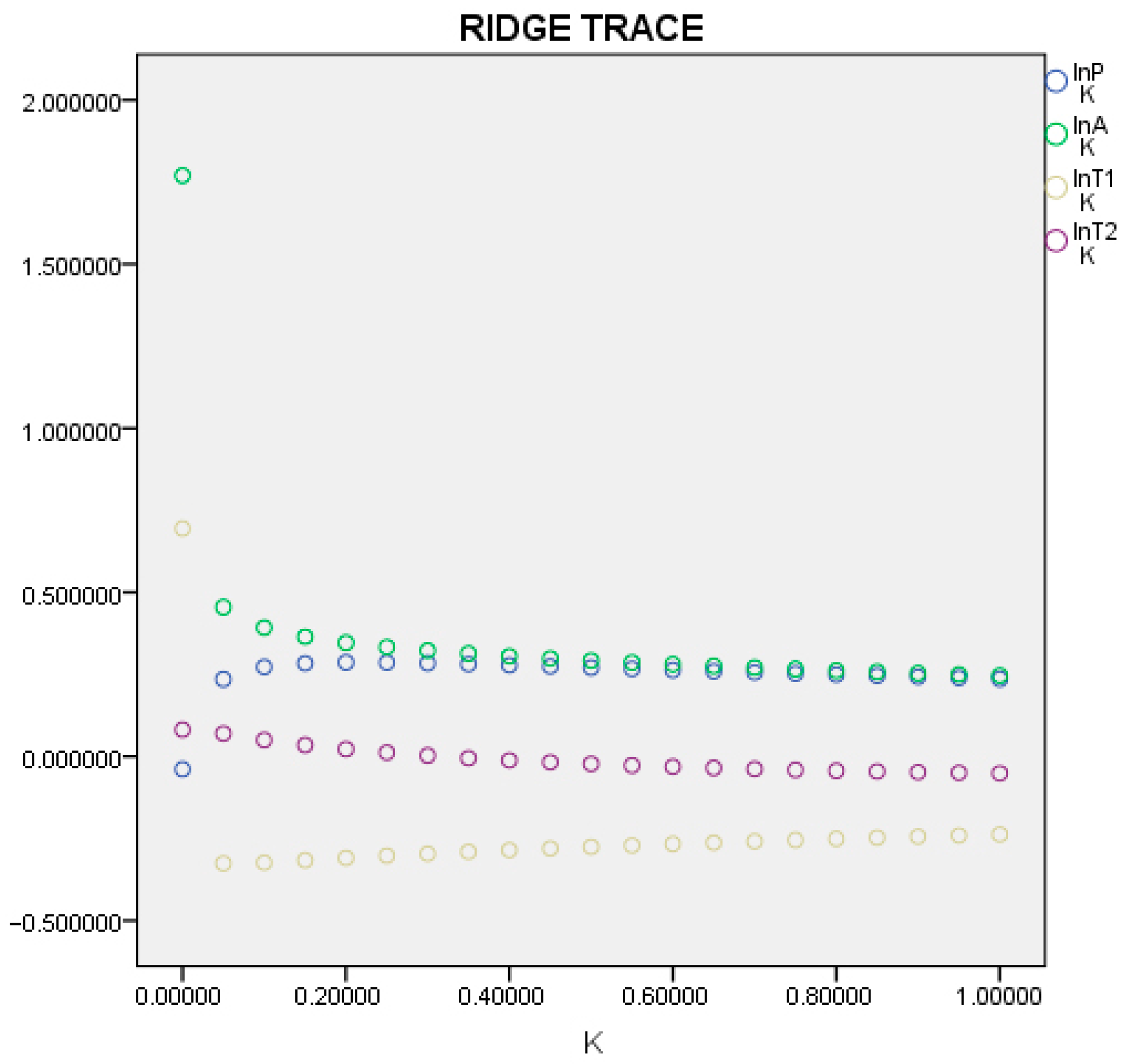
2.2. Ridge Regression

Ridge regression (RR) is a biased estimation regression method that is used exclusively for collinearity data analysis [29]. In essence, it is an improved least square estimation method. RR is a more realistic and reliable regression method to get the regression coefficient by giving up unbiased characteristics, losing some information and reducing accuracy [30]. The fitting of RR to ill conditioned data is better than that of least squares [31]. For the multivariate linear regression model $Y=X\beta +\epsilon$, the least-squares estimator of parameter $\beta$ is:

$$\widehat{\beta }={(X\prime X)}^{-1}X\prime Y$$

(3)

However, when the multicollinearity exists, the least square parameter estimation is singular. Some characteristic roots are close to 0, and there is a large deviation between the estimated values and the observed ones. Thus, the traditional least squares estimation is not reliable enough. And RR adjusts the estimate to:

$$\widehat{\beta }(k)={(X\prime X+kI)}^{-1}X\prime Y$$

(4)

where I represents the unit matrix, k is the ridge parameter. When k = 0, the ridge estimate $\widehat{\beta }(0)$ is the least-squares estimation. When k varies between $[0,\infty )$, $\widehat{\beta }(k)$ is a function of the ridge parameter k. Multiple function curves are plotted in a graph as a ridge plot. Finally, the k value which makes the $\widehat{\beta }(k)$ value stable is chosen as the ridge parameter.

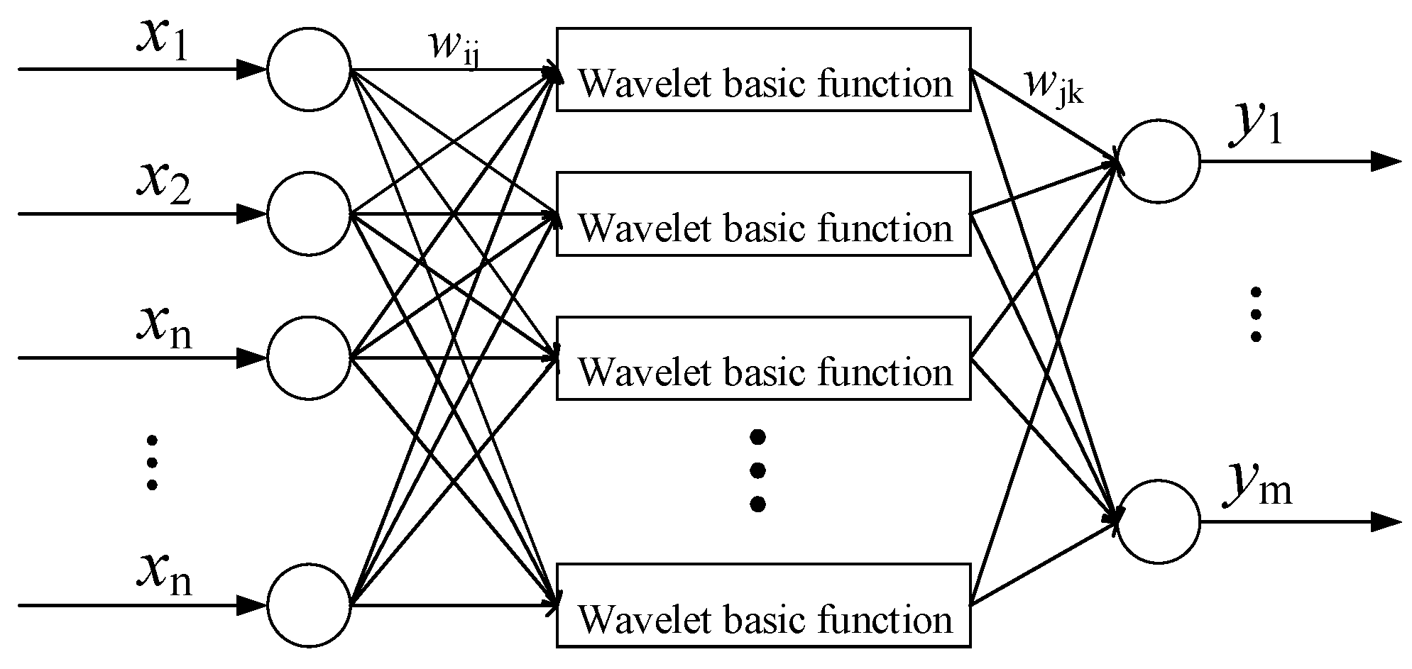
2.3. Wavelet Neural Network Prediction Model

Wavelet Neural Network (WNN) is a new type of feed-forward network, which combines the wavelet transform with neural networks and uses the nonlinear wavelet base function as the transfer function in the hidden layer, which is able to realize signals forward-propagation and error back-propagation simultaneously [32,33]. The wavelet function is obtained by the translation and expansion of its mother wavelet, and the signal can be decomposed into a series of wavelet functions [34]. After shifting the base wavelet function $\psi (t)$ by $\tau$, multiply it with the target signal at different scales, namely:

$$f_x(a,\tau )=\frac{1}{\sqrt{a}}{\displaystyle {\int }_{-\infty }^{\infty }x(t)\psi (\frac{t-\tau }{a}})dt,a>0$$

(5)

where $\tau$ represents the parallel movement of the target, a refers to adjusting the distance from the target. The graph of WNN structure is illustrated in Figure 1.

Where x₁, x₂, …, x_n represent the input value of WNN, y₁, y₂, …, y_m represent the output value of WNN, weight values are w_ij and w_jk. The output of the hidden layer is:

$$h(j)=h_j\left(\frac{{\displaystyle \sum _{i=1}^k{w}_{ij}{x}_i-b_j}}{a_j}\right),j=1,2,\cdots ,l$$

(6)

The output of the hidden layer node $j$ is $h(j)$, w_ij is the weight of the input and the hidden layer, the translation factor of the wavelet basis function $h_j$ is expressed by $b_j$, and the scaling factor is expressed by $a_j$. The output layer is calculated as:

$$y(k)={\displaystyle \sum _{j=1}^l{w}_{jk}h(j)},k=1,2,\cdots ,m$$

(7)

where w_jk is the weight of the input layer and the hidden layer.

WNN is also able to keep the neural network close to the expected data output by gradient modifying parameters of the base wavelet function and the neural network weights [35]. Assume that the network error is e, the expected output is $yn(k)$, and the actual prediction value is $y(k)$, namely,

$$e={\displaystyle \sum _{k=1}^{m}yn(k)-y(k)}$$

(8)

Then the following equations can be obtained.

$$\Delta w^{i+1}=-\mu \frac{\partial e}{\partial w^i}$$

(9)

$$\Delta b^{i+1}=-\mu \frac{\partial e}{\partial b^i}$$

(10)

$$\Delta a^{i+1}=-\mu \frac{\partial e}{\partial a^i}$$

(11)

where $\mu$ represents the learning rate, and the revised parameters can be obtained by plugging $\mu$ into the following formulas.

$$w^{i+1}=w^i+\Delta w^{i+1}$$

(12)

$$b^{i+1}=b^i+\Delta b^{i+1}$$

(13)

$$a^{i+1}=a^i+\Delta a^{i+1}$$

(14)

2.4. Gauss Optimized Cuckoo Search Algorithm

2.4.1. Cuckoo Search Algorithm

The Cuckoo Search (CS) algorithm can search the optimization much faster and more accurately by simulating the cuckoo searching for the random walking process of the egg laying hosts [36]. According to Yang et al.’s research, the Cuckoo Search algorithm has the following three rules [37]:

(1)

The number of eggs produced by a cuckoo per time is 1.

(2)

The host bird’s nest where high-quality eggs are located is the optimal solution and will be retained for the next generation.

(3)

The number of host nests is certain, and the probability that cuckoo eggs are found by nest owners is $P_a\in \left[0,1\right]$.

During the search, cuckoo’s flight search path follows the Lévy distribution [38,39], namely:

$$x_i^{(t+1)}=x_i^{(t)}+\alpha \oplus L(\lambda ),i=1,2,\cdots ,n$$

(15)

In the formula, $x_i^{(t+1)}$ and $x_i^{(t)}$ are the bird’s nest positions of the (t + 1)-th and the t-th generation, n is the number of cuckoo, $\oplus$ is the dot multiplication and $L(\lambda )$ is the Lévy flight path. The relation between searching path and time is as follows:

$$L(\lambda )\sim u=t^{-\lambda }(1<\lambda \le 3)$$

(16)

2.4.2. Gauss Optimization

In the traditional CS algorithm, the probability of finding cuckoo eggs and the step size $\alpha$ of position updating are fixed values, which leads to the problems of the weak global search ability, slow convergence speed and low precision of the algorithm [40]. Therefore, an improved cuckoo algorithm is proposed in this paper to update the values of $P_a$ and $\alpha$ dynamically. According to references, where the updating process is as follows:

$$P_a(t)=P_{a\max }-\frac{t(P_{a\max }-P_{a\min })}{N}$$

(17)

$$\alpha (t)={\alpha }_{\max }{e}^{\frac{\ln (\frac{{\alpha }_{\max }}{{\alpha }_{\min }})\times t}{N}}$$

(18)

In the formula, t and N are the number of current iterations and the total number of iterations, $P_{a\max }$ and $P_{a\min }$ are the maximum and minimum values of the detection probability, ${\alpha }_{\max }$ and ${\alpha }_{\min }$ are the maximum and minimum step coefficients, respectively.

However, due to the lack of search vitality and slow speed of CS algorithm, the optimization ability of CS algorithm can be improved effectively by adding Gauss perturbation. Assuming that the optimal location of the nest $x_i^{(i)}$, ($i=1,2,\cdots ,n$), is obtained after the calculation of t times CS iterations. In order to prevent the next iteration of $x_i^{(i)}$ and maintain the Gaussian disturbance, the next phase of $x_i^{(i)}$ is searched. Supposed that the matrix $p_t={[x_1^{(t)},x_2^{(t)},\cdots ,x_n^{(t)}]}^r$ is made up of the better position $x_i^{(i)}$ of the bird’s nest, $x_i^{(i)}$ is a d-dimensional vector, and the dimension of $p_t$ is $d\times n$. Matrix $p_t$ combined with Gaussian perturbation is the basic step of GCS algorithm [41], namely:

$$p_t=p_t+a\oplus \epsilon$$

(19)

where $\epsilon$ is a random matrix with the same order of $p_t$, which follows N(0, 1) distribution and a is constant. In the search for a better nest position vitality at the same time, the position of the bird’s nest can be overextended easily because of the large random range of $\epsilon$.

Therefore, the selection of suitable a is particularly important. After obtaining a reasonable set of $p_t\prime$ and comparing it with each nest in $p_t$, only a better nest position is reserved to obtain a better set of nest positions $p_t\prime$.

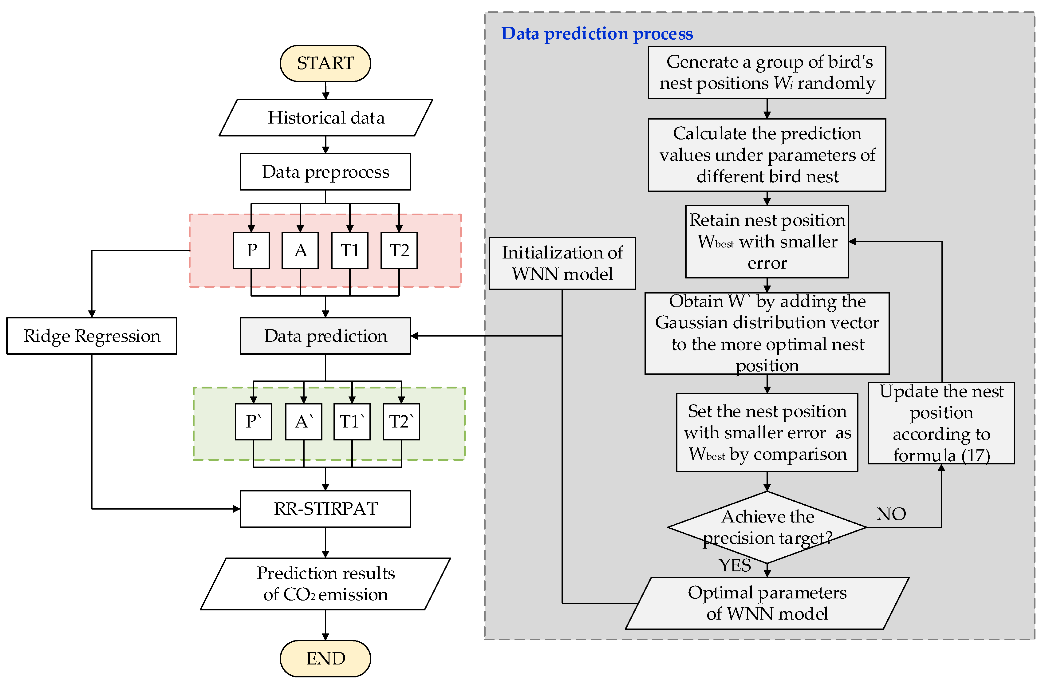
2.5. The Prediction Model of RR-STIRPAT-GCS-WNN

The emission of CO₂ in power generation industry is mainly affected by population, per capita GDP, standard coal consumption, proportion of thermal power and other factors. The forecasting steps are as follow:

(1) Data collecting and processing

Collect the historical data of population, per capita GDP, standard coal consumption, proportion of thermal power from 1996–2016.

(2) Establish regression model

Use the logarithm of historical data to establish regression model between the influencing factors and the CO₂ emission in power generation industry based on STIRPAT by ridge regression method.

(3) Prediction model training

Initialize parameters of prediction model. The input layer node is set as 2, while the hidden layer node is 2 × 2 + 1 = 5, and the output layer node is 1. The weight value, translation factor and expansion factor of the wavelet base are randomly generated. In this study, the learning rate is set as 0.1, while the number of iterations is 500, and the prediction accuracy is 0.99.

Then train the prediction model by plugging the historical data into the model and search the best parameter by using the Gauss Optimized Cuckoo Search Algorithm. Firstly, set the N_nest (number of birds’ nest) as 30, while P_a (probability of bird’s eggs by bird’s nest owner) is 0.2, and N (number of iterations) is 200. After that, randomly generate N_nest bird nest location W = (W₁, W₂, ..., N_nest) ^T. And each bird nest W_i has s parameters (s = the number of weights between input layer and hidden layer + the number of weights between hidden layer and output layer + the number of translation factors + the number of expansion factors). The predicted values of each bird’s nest were calculated, and the nest which has the smallest error in the 30 nests is found, marked as W_best. Then W_best retain to the next generation.

(4) Prediction of CO₂ Emission

Use the RR-STIRPAT-GCS-WNN model to forecast the CO₂ Emission in Power generation industry based on the historical data of population, per capita GDP, standard coal consumption and proportion of thermal power. The flow chart of this model is shown in the Figure 2.

3. Results

3.1. Analysis on Influencing Factors of CO₂ Emission in Power Generation Industry

Based on the scholars’ research on the influencing factors of CO₂ emission in power generation industry and the basic framework of STIRPAT model, 4 factors, such as population scale (million people), per capita GDP (yuan), standard coal consumption (g/kWh), and thermal power specific gravity (%), are considered as the key factors affecting the CO₂ emission from the power generation industry. The above factors are introduced into the STIRPAT model:

$$\ln I=a+b\ln P+c\ln A+d\ln T_1+e\ln T_2+f$$

(20)

where I represents CO₂ annual emissions, P means population size, A is per capita GDP, T₁ is power supply standard coal consumption, T₂ is proportion of thermal power, b, c, d, e are various coefficients. According to the concept of elasticity, b, c, d and e represent the elastic coefficients of each index when both sides of the equation take partial derivatives at the same time. The raw data is shown in

Table 1. Raw data.

Year	CO2 Annual Emissions (million tons)	Population (million people)	Per Capita GDP (yuan)	Standard Coal Consumption (g/kWh)	Proportion of Thermal Power
1995	915.36	1211.21	5091	412	0.795
1996	1005.78	1223.89	5898	410	0.813
1997	1022.69	1236.26	6481	408	0.815
1998	1021.78	1247.61	6860	404	0.795
1999	1053.64	1257.86	7229	399	0.798
2000	1082.86	1267.43	7942	392	0.822
2001	1145.20	1276.27	8717	385	0.799
2002	1300.08	1284.53	9506	383	0.809
2003	1542.09	1292.27	10,666	380	0.827
2004	1822.60	1299.88	12,487	376	0.815
2005	2036.69	1307.56	14,368	370	0.819
2006	2321.18	1314.48	16,738	367	0.827
2007	2538.77	1321.29	20,505	356	0.830
2008	2625.22	1328.02	24,121	345	0.805
2009	2793.57	1334.50	26,222	340	0.803
2010	3099.39	1340.91	30,876	333	0.792
2011	3537.78	1347.35	36,403	329	0.813
2012	3600.12	1354.04	40,007	326	0.781
2013	3749.21	1360.72	43,852	321	0.789
2014	3904.66	1367.82	47,203	318	0.752
2015	4042.31	1374.62	50,251	318	0.737
2016	4162.96	1382.71	53,817	312	0.716

.

According to the data in the table, after taking the logarithm of the indicators, SPSS software is used to achieve the least squares regression model based on STIRPAT. The regression results are shown in

Table 2. Model Summary.

Model	R	R2	Adjusted R2	Std. Error of the Estimate
1	0.996	0.992	0.991	0.05326

,

Table 3. ANOVA.

Model		Sum of Squares	df	Mean Square	F	Significance (Sig.)
1	Regression	6.299	4	1.575	555.098	0.000
	Residual	0.048	17	0.003
	Total	6.347	21

and

Table 4. Coefficients.

Model		Unstandardized Coefficients		Standardized Coefficients	t	Sig.	Collinearity Statistics
		B	Std. Error	Beta			Tolerance	VIF
1	(Constant)	−16.678	21.648		−0.770	0.452
	ln P	−0.547	1.529	−0.039	−0.358	0.725	0.038	26.232
	ln A	1.227	0.205	1.770	5.995	0.000	0.005	194.998
	ln T1	4.020	1.665	0.695	2.413	0.027	0.005	185.319
	ln T2	1.191	0.424	0.081	2.813	0.012	0.533	1.878

.

According to the regression results, the regression coefficient of the model is 0.992, the adjustment coefficient is 0.991, and the F value is 555.098. It shows that the equation passed the significance test and the fitting effect is good. However, the variance expansion factor VIF is greater than 10 except for ln T₂, indicating the possibility of multicollinearity. Therefore, the collinearity tests were performed, and the results are shown in

Table 5. Collinearity diagnosis.

Model	Dimension	Eigenvalue	Condition Index	Variance Proportions
				(Constant)	ln P	ln A	ln T1	ln T2
1	1	4.976	1.000	0.00	0.00	0.00	0.00	0.00
	2	0.020	15.721	0.00	0.00	0.00	0.00	0.48
	3	0.004	36.975	0.00	0.00	0.01	0.00	0.33
	4	9.050 × 10−7	2344.946	0.03	0.15	0.98	0.79	0.03
	5	1.718 × 10−7	5382.577	0.97	0.85	0.01	0.21	0.15

.

According to the result of collinearity diagnosis, 4 of the 5 eigenvalues are close to 0, the maximum condition number is 5382.577. It is shown that the equation has multicollinearity characteristics. In order to solve the problem of multicollinearity without reducing the number of variables, the ridge regression method is applied to solve the multiple collinearity considering the few variables of the model. The ridge trace is shown in Figure 3.

It can be seen from the above figure that when k = 0.4, the ridge parameter is basically stable, at this time R² is still relatively large. Therefore, k = 0.4 is determined as ridge parameter for regression. Ridge regression results are shown in

Table 6. Ridge Regression with k = 0.4.

Mult R	R2	Adjusted R2	SE
0.9801579272	0.9607095623	0.9514647534	0.1211139063

,

Table 7. ANOVA.

	df	SS	MS	F Value	Sig. F
Regress	4.000	6.097	1.524	103.9188127	0.0000000
Residual	17.000	0.249	0.015

and

Table 8. Variables in the Equation.

	B	SE(B)	Beta	B/SE(B)
ln P	3.92423625	0.30690079	0.27792333	12.78666051
ln A	0.21204247	0.01169894	0.30586681	18.12492455
ln T1	−1.65055241	0.09696411	−0.28521636	−17.02230296
ln T2	−0.16815311	0.51870654	−0.01150223	−0.32417772
Constant	−26.39759673	3.47936456	0.00000000	−7.58690166

.

As can be seen from the above table, R² = 0.9607 and F = 103.9188 at k = 0.4, the equation passes the significance test and no longer exists multicollinearity. It shows that the model established by ridge regression is reasonable, and the regression equation is as follows:

$$\ln I=3.9242\ln P+0.212\ln A-1.6506\ln T_1-0.1682\ln T_2-26.3976$$

(21)

3.2. Prediction of CO₂ Emission in Power Generation Industry

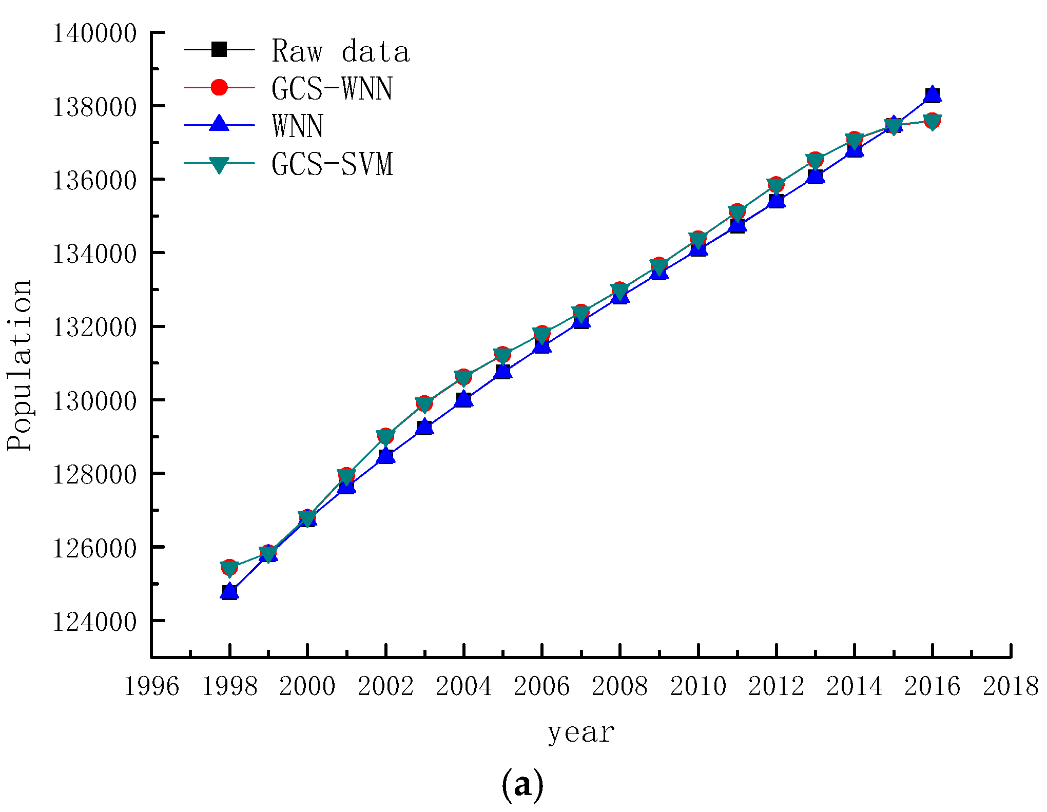
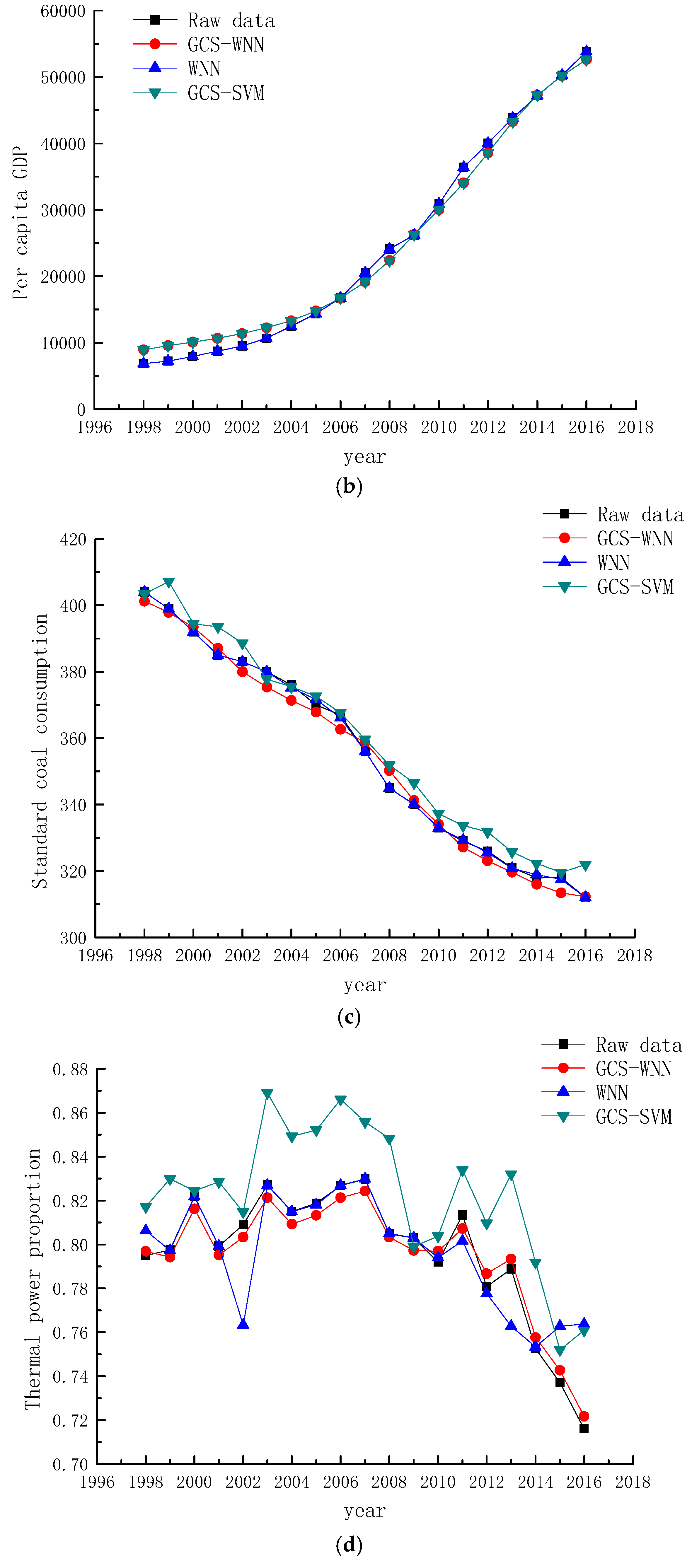
3.2.1. Prediction of Influencing Factors Based on GCS-WNN

Based on the historical data of population, per capita GDP, standard coal consumption and proportion of thermal power from 1995 to 2016, historical data were trained and predicted by using GCS-WNN model, WNN model and GCS-SVM model respectively. The prediction results are shown in Figure 4.

By comparing the model predictions in Figure 4, it can be seen that the prediction accuracy of the GCS-WNN model is the highest among all the indicators, which is basically consistent with the original data. Therefore, the GCS-WNN model can be used to predict the future population, per capita GDP, standard coal consumption, proportion of thermal power and other indicators.

The prediction results of CO₂ emission were obtained by plugging the predicted values of each influencing factor into the established RR-STIRPAT model. The prediction results are shown in the Figure 5.

According to the Figure 5 and Figure 6, the prediction accuracy of GCS-WNN model is the highest, which has best fitting effect with the original data. It shows that the RR-STIRPAT-GCS-WNN model is accurate and scientific in the prediction of CO₂ emission.

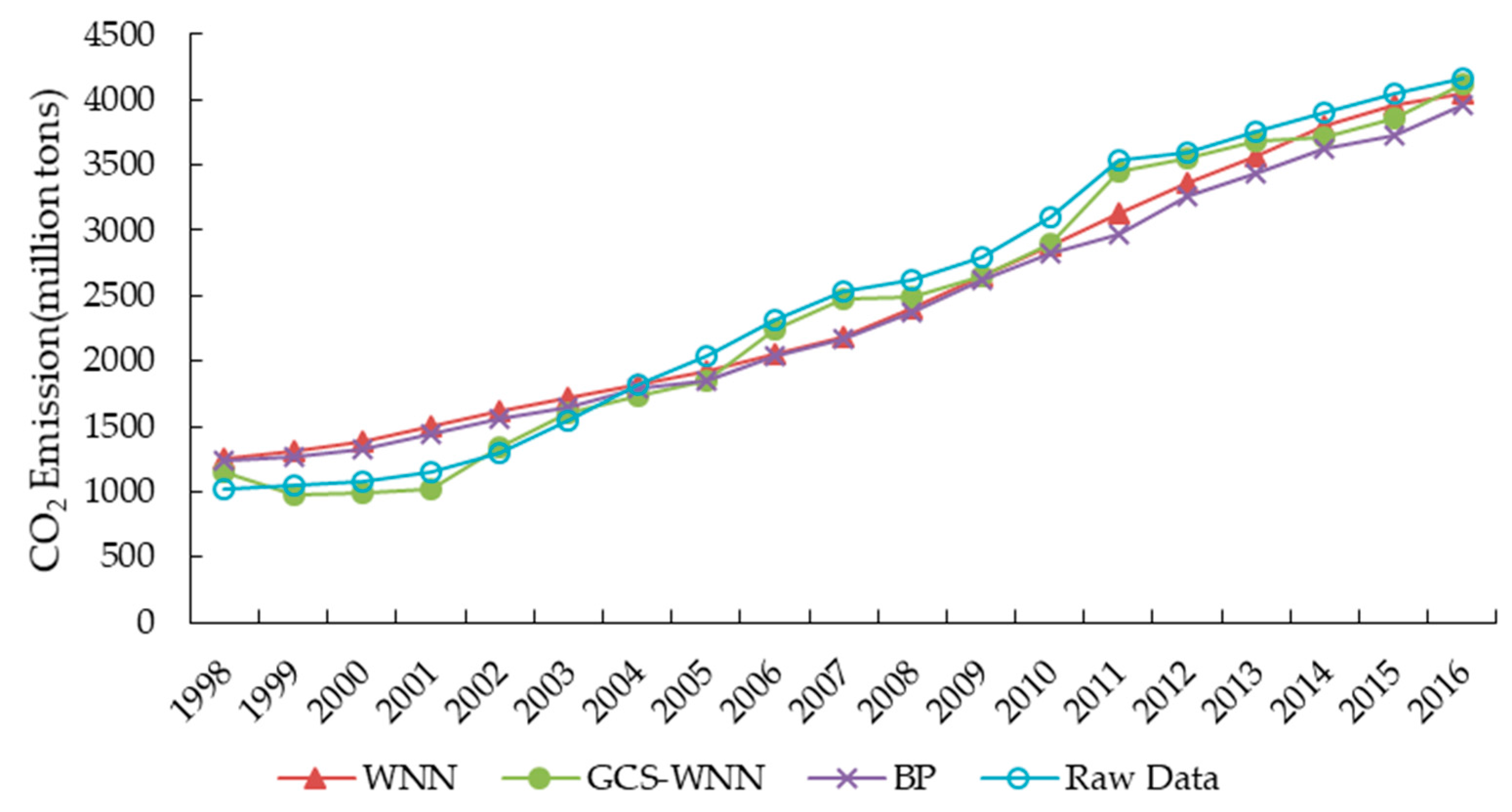
3.2.2. Prediction of CO₂ Emission Based on RR-STIRPAT Model

On the basis of historical data, GCS-WNN is used to predict 2018–2022 years population, per capita GDP, standard coal consumption, proportion of thermal power and other indicators. The results are shown in

Table 9. Prediction results of influencing factors.

Year	Population (million people)	Per Capita GDP (yuan)	Standard Coal Consumption (g/kWh)	Proportion of Thermal Power
2018	1379.12	59,894	307.4795	0.6879
2019	1380.15	61,761	304.9642	0.6698
2020	1381.56	64,597	301.4681	0.6514
2021	1383.69	66,717	299.1497	0.6498
2022	1385.14	69,486	297.3476	0.6389

.

The prediction results of CO₂ emissions in power generation industry in 2018–2022 years could be obtained by plugging the results of each factor into the RR-STIRPAT model. The prediction results are shown in

Table 10. Prediction of CO₂ emission.

Year	CO2 (Unit: million tons)
2018	4347.48
2019	4468.63
2020	4638.16
2021	4760.55
2022	4883.71

and Figure 7.

It can be seen from the Table 10 and Figure 7 that during the period of 2018–2022, the CO₂ emissions from the power generation industry will still keep rising. However, the growth rate of CO₂ emission will continue to decline due to the slowdown of population growth, the drop of standard coal consumption and the decrease of the proportion of thermal power in the future.

4. Discussion and Conclusions

Greenhouse gas emissions, represented by CO₂, have led to a rise in global temperatures. Power generation industry is one of the key industries of CO₂ emissions. To achieve the purpose of controlling CO₂ emissions, it is necessary to scientifically and quantitatively predict the CO₂ emissions of power generation industry.

(1)

The CO₂ emission of power generation industry is affected by many factors. It is concluded that the key factors that directly affect CO₂ emissions are population, per capita GDP, standard coal consumption and proportion of thermal power.

(2)

Based on the STIRPAT model, the CO₂ emission factors analysis model of power generation industry is established. Besides, the collinearity test of the model shows that if the ordinary least squares algorithm is applied, the multicollinearity will be serious. However, the ridge regression method can solve this problem to a certain extent.

(3)

The WNN model is used to predict the influencing factors. In order to improve the convergence speed and prediction accuracy of the model, Gauss optimized cuckoo search algorithm is added into the model parameter optimization. Compared with other models, it is found that the optimized model has higher prediction accuracy.

(4)

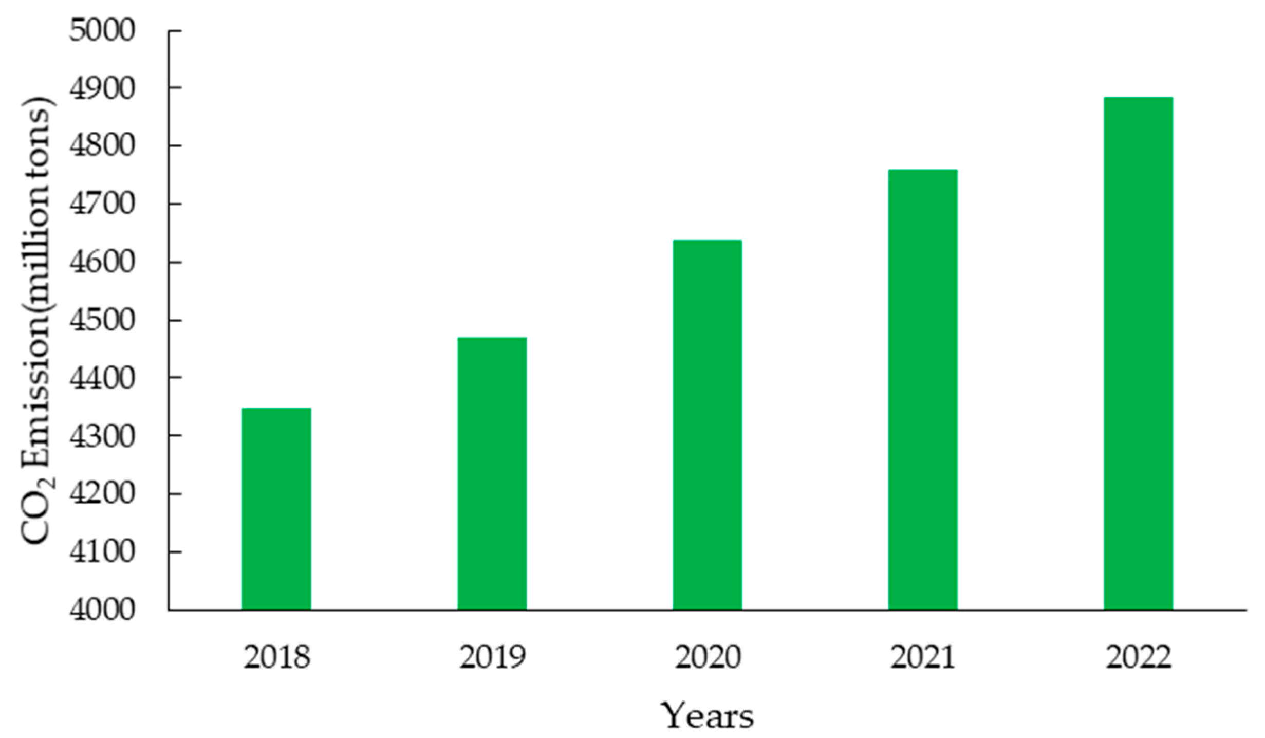
The GCS-WNN model is used to predict the population, per capita GDP, standard coal consumption and the proportion of thermal power in the past 2018–2022 years. The predicted results of each factor are plugged into the RR-STIRPAT model, and finally the CO₂ emission prediction value of 2018–2022 years power generation industry is obtained. It is predicted that the CO₂ emission from the power generation industry will increase gradually in the next five years. However, with the slowdown of population growth and the development of power generation technology, CO₂ emissions in power generation industry will grow slower and slower.

The advantages of the prediction model in this paper includes that the prediction precision is much higher and more scientific factors are taken into account. But limited to the availability of data, the factors considered in this study are not all-round, which also restricts the application of intelligent algorithms. In future research, we will continue to explore more accurate prediction methods and propose more scientific prediction models.

References

1. The Electric Power Development Planning “in 13th Five-Year” (2016–2020 (Full Text). Available online: http://news.bjx.com.cn/html/20161222/798873.shtml (accessed on 22 December 2016).
2. Liu, L.; Zong, H.; Zhao, E.; Chen, C.; Wang, J. Can China realize its carbon emission reduction goal in 2020: From the perspective of thermal power development. Appl. Energy 2014, 124, 199–212. [Google Scholar] [CrossRef]
3. Seo, Y.; Ide, K.; Kitahata, N.; Kuchitsu, K.; Dowaki, K. Environmental Impact and Nutritional Improvement of Elevated CO2 Treatment: A Case Study of Spinach Production. Sustainability 2017, 9, 1854. [Google Scholar] [CrossRef]
4. Shahbaz, M.; Loganathan, N.; Muzaffar, A.T.; Ahmed, K.; Jabran, M.A. How urbanization affects CO2, emissions in Malaysia? The application of STIRPAT model. Renew. Sustain. Energy Rev. 2016, 57, 83–93. [Google Scholar] [CrossRef]
5. Wang, C.; Wang, F.; Zhang, X.; Yang, Y.; Su, Y.; Ye, Y.; Zhang, H. Examining the driving factors of energy related carbon emissions using the extended STIRPAT model based on IPAT identity in Xinjiang. Renew. Sustain. Energy Rev. 2017, 67, 51–61. [Google Scholar] [CrossRef]
6. Shahbaz, M.; Chaudhary, A.R.; Ozturk, I. Does urbanization cause increasing energy demand in Pakistan? Empirical evidence from STIRPAT model. Energy 2017, 122, 83–93. [Google Scholar] [CrossRef]
7. Shuai, C.; Shen, L.; Jiao, L.; Wu, Y.; Tan, Y. Identifying key impact factors on carbon emission: Evidences from panel and time-series data of 125 countries from 1990 to 2011. Appl. Energy 2017, 187, 310–325. [Google Scholar] [CrossRef]
8. Wang, P.; Wu, W.; Zhu, B.; Wei, Y. Examining the impact factors of energy-related CO2 emissions using the STIRPAT model in Guangdong Province, China. Appl. Energy 2013, 106, 65–71. [Google Scholar] [CrossRef]
9. Li, W.; Sun, S. Air pollution driving factors analysis: Evidence from economically developed area in China. Environ. Prog. Sustain. Energy 2016, 35, 1231–1239. [Google Scholar] [CrossRef]
10. Al-Mulali, U.; Fereidouni, H.G.; Lee, J.Y.M.; Normee Che Sab, C. Exploring the relationship between urbanization, energy consumption, and CO2 emission in MENA countries. Renew. Sustain. Energy Rev. 2013, 23, 107–112. [Google Scholar] [CrossRef]
11. Zhang, C.; Liu, C. The impact of ICT industry on CO2 emissions: A regional analysis in China. Renew. Sustain. Energy Rev. 2015, 44, 12–19. [Google Scholar] [CrossRef]
12. Xie, C.; Hawkes, A.D.; Lund, H. Estimation of inter-fuel substitution possibilities in China’s transport industry using ridge regression. Energy 2015, 88, 260–267. [Google Scholar] [CrossRef]
13. Yue, Y.; Li, M.; Zhu, A.X.; Ye, X.; Mao, R.; Wan, J.; Dong, J. Land Degradation Monitoring in the Ordos Plateau of China Using an Expert Knowledge and BP-ANN-Based Approach. Sustainability 2016, 8, 1174. [Google Scholar] [CrossRef]
14. Kumar, U.; Jain, V.K. Time series models (Grey-Markov, Grey Model with rolling mechanism and singular spectrum analysis) to forecast energy consumption in India. Energy 2010, 35, 1709–1716. [Google Scholar] [CrossRef]
15. Li, S.; Li, R. Comparison of forecasting energy consumption in Shandong, China Using the ARIMA model, GM model, and ARIMA-GM model. Sustainability 2017, 9, 1181. [Google Scholar] [CrossRef]
16. Xu, J.; Ren, Q.; Shen, Z. Prediction of the strength of concrete radiation shielding based on LS-SVM. Ann. Nucl. Energy 2015, 85, 296–300. [Google Scholar]
17. Gao, Y.; Cheng, H.; Zhu, J.; Liang, H.; Li, P. The Optimal Dispatch of a Power System Containing Virtual Power Plants under Fog and Haze Weather. Sustainability 2016, 8, 71. [Google Scholar] [CrossRef]
18. Nieto, P.J.G.; García-Gonzalo, E.; Fernández, J.R.A.; Díaz Muñizb, C. A hybrid PSO optimized SVM-based model for predicting a successful growth cycle of the Spirulina platensis, from raceway experiments data. Ecol. Eng. 2015, 81, 534–542. [Google Scholar] [CrossRef]
19. Kim, H.; Baek, S.; Choi, K.; Kim, D.; Lee, S.; Kim, D.; Chang, H.J. Comparative Analysis of On- and Off-Grid Electrification: The Case of Two South Korean Islands. Sustainability 2016, 8, 350. [Google Scholar] [CrossRef]
20. Zhang, F.; Dong, Y.; Zhang, K. A Novel Combined Model Based on an Artificial Intelligence Algorithm—A Case Study on Wind Speed Forecasting in Penglai, China. Sustainability 2016, 8, 555. [Google Scholar] [CrossRef]
21. Gao, C.; Wang, K. Micro-grid power forecast based on MSC-WNN model. Electr. Meas. Instrum. 2015, 52, 68–73. [Google Scholar]
22. Wang, Z.; Wang, C.; Wu, J. Wind Energy Potential Assessment and Forecasting Research Based on the Data Pre-Processing Technique and Swarm Intelligent Optimization Algorithms. Sustainability 2016, 8, 1191. [Google Scholar] [CrossRef]
23. York, R.; Rosa, E.A.; Dietz, T. STIRPAT, IPAT and ImPACT: Analytic tools for unpacking the driving forces of environmental impacts. Ecol. Econ. 2003, 46, 351–365. [Google Scholar] [CrossRef]
24. Yu, X.; Geng, Y.; Dong, H.; Ulgiati, S.; Liu, Z.; Liu, Z.; Ma, Z.; Tian, X.; Sun, L. Sustainability assessment of one industrial region: A combined method of emergy analysis and IPAT (Human Impact Population Affluence Technology). Energy 2016, 107, 818–830. [Google Scholar] [CrossRef]
25. Dong, J.F.; Wang, Q.; Deng, C.; Wang, X.-M.; Zhang, X.-L. How to Move China toward a Green-Energy Economy: From a Sector Perspective. Sustainability 2016, 8, 337. [Google Scholar] [CrossRef]
26. Zhang, Z.; Chen, X.; Heck, P. Emergy-Based Regional Socio-Economic Metabolism Analysis: An Application of Data Envelopment Analysis and Decomposition Analysis. Sustainability 2014, 6, 8618–8638. [Google Scholar] [CrossRef]
27. Liu, Y.; Yang, Z.; Wu, W. Assessing the impact of population, income and technology on energy consumption and industrial pollutant emissions in China. Appl. Energy 2015, 155, 904–917. [Google Scholar] [CrossRef]
28. Li, K.; Lin, B. Impacts of urbanization and industrialization on energy consumption/CO2, emissions: Does the level of development matter? Renew. Sustain. Energy Rev. 2015, 52, 1107–1122. [Google Scholar] [CrossRef]
29. Marquardt, D.W.; Snee, R.D. Ridge Regression in Practice. Am. Stat. 1975, 29, 3–20. [Google Scholar]
30. Hoerl, A.E.; Kennard, R.W. Ridge Regression: Applications to Nonorthogonal Problems. Technometrics 1970, 12, 69–82. [Google Scholar] [CrossRef]
31. Hoerl, A.E.; Kennard, R.W. Ridge Regression: Biased Estimation for Nonorthogonal Problems. Technometrics 2000, 42, 80–86. [Google Scholar] [CrossRef]
32. Feng, Y.; Cui, N.; Zhao, L.; Hu, X.; Gong, D. Comparison of ELM, GANN, WNN and empirical models for estimating reference evapotranspiration in humid region of Southwest China. J. Hydrol. 2016, 536, 376–383. [Google Scholar] [CrossRef]
33. Ganjefar, S.; Tofighi, M. Single-hidden-layer fuzzy recurrent wavelet neural network: Applications to function approximation and system identification. Inf. Sci. 2015, 294, 269–285. [Google Scholar] [CrossRef]
34. Wang, W.; Zhang, M.; Liu, X. Improved fruit fly optimization algorithm optimized wavelet neural network for statistical data modeling for industrial polypropylene melt index prediction. J. Chemometr. 2015, 29, 506–513. [Google Scholar] [CrossRef]
35. Kasiviswanathan, K.S.; He, J.; Sudheer, K.P.; Tay, J.-H. Potential application of wavelet neural network ensemble to forecast streamflow for flood management. J. Hydrol. 2016, 536, 161–173. [Google Scholar] [CrossRef]
36. Walton, S.; Hassan, O.; Morgan, K.; Brown, M.R. Modified cuckoo search: A new gradient free optimisation algorithm. Chaos Solitons Fract. 2011, 44, 710–718. [Google Scholar] [CrossRef]
37. Ahmed, J.; Salam, Z. A Maximum Power Point Tracking (MPPT) for PV system using Cuckoo Search with partial shading capability. Appl. Energy 2014, 119, 118–130. [Google Scholar] [CrossRef]
38. Nguyen, T.T.; Vo, D.N.; Truong, A.V. Cuckoo search algorithm for short-term hydrothermal scheduling. Appl. Energy 2014, 132, 276–287. [Google Scholar] [CrossRef]
39. Li, X.T.; Yin, M.H. A hybrid cuckoo search via Lévy flights for the permutation flow shop scheduling problem. Int. J. Prod. Res. 2013, 51, 732–4754. [Google Scholar] [CrossRef]
40. Zheng, H.; Zhou, Y. A novel Cuckoo Search optimization algorithm base on gauss distribution. J. Comput. Inf. Syst. 2012, 8, 4193–4200. [Google Scholar]
41. Lai, J.; Liang, S.; Center, C. Application of GCS-SVM model in network traffic prediction. Comput. Eng. Appl. 2013, 49, 75–78. [Google Scholar]
Figure 1. Wavelet Neural Network (WNN) structure.
Sustainability 09 02377 g001
Figure 2. The flow chart of ridge regression Stochastic Impacts by Regression on Population, Affluence and Technology Gauss Cuckoo Search Wavelet Neural Network (RR-STIRPAT-GCS-WNN) model.
Sustainability 09 02377 g002
Figure 3. Ridge Trace.
Sustainability 09 02377 g003
Figure 4. Prediction results. (a) Prediction results of population; (b) Prediction results of per capita GDP; (c) Prediction results of standard coal consumption; (d) Prediction results of thermal power proportion.
Sustainability 09 02377 g004aSustainability 09 02377 g004b
Figure 5. Prediction results of CO2 emission.
Sustainability 09 02377 g005
Figure 6. Error boxplot of different models.
Sustainability 09 02377 g006
Figure 7. Prediction of CO2 emission.
Sustainability 09 02377 g007