Application of Source-Sink Landscape Influence Values to Commuter Traffic: A Case Study of Xiamen Island


Abstract
:1. Introduction
2. Materials
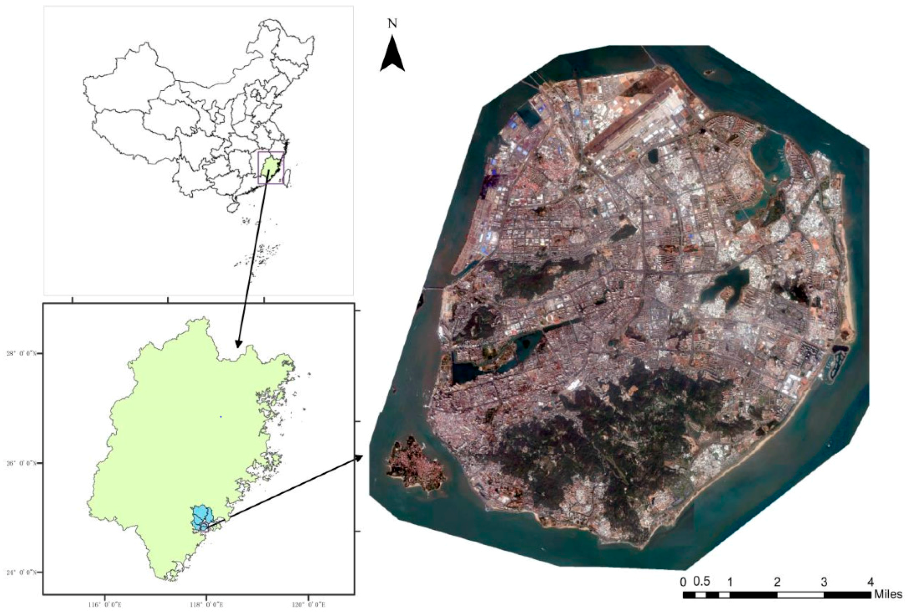
2.1. Research Area
2.2. Data Source
3. Methods
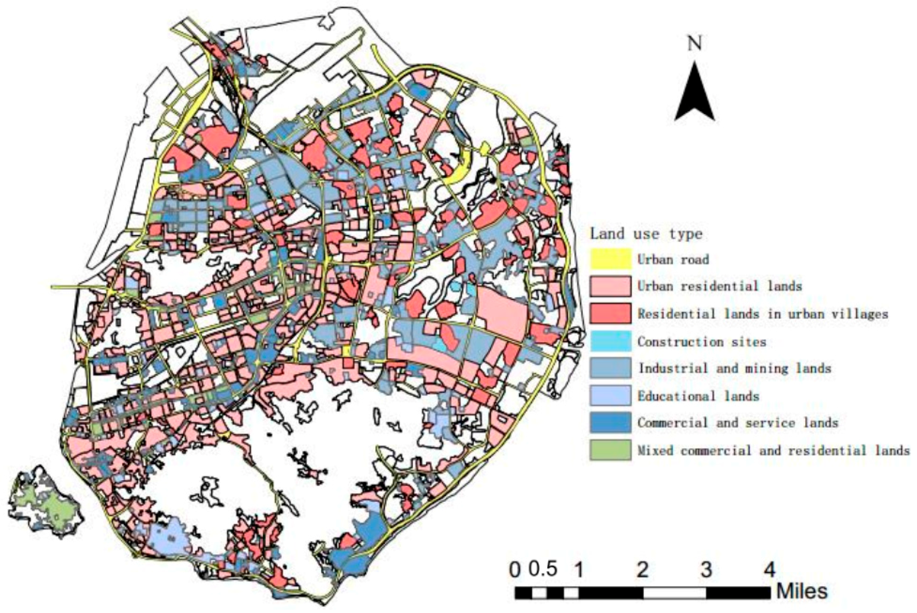
3.1. Land Use Classification
3.2. TRANUS Modeling
3.3. Source-Sink Landscape Theory
3.3.1. Source-Sink Landscape Classification
3.3.2. Source-Sink Landscape Influence
4. Results
4.1. Values of Source-Sink Landscape Influence
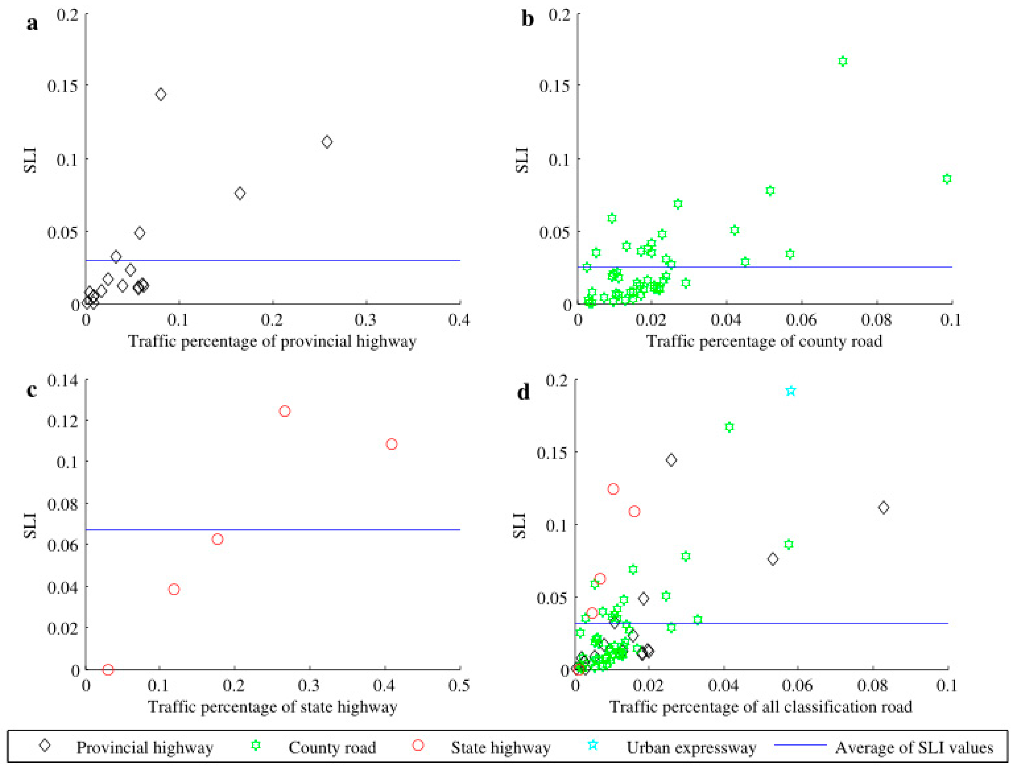
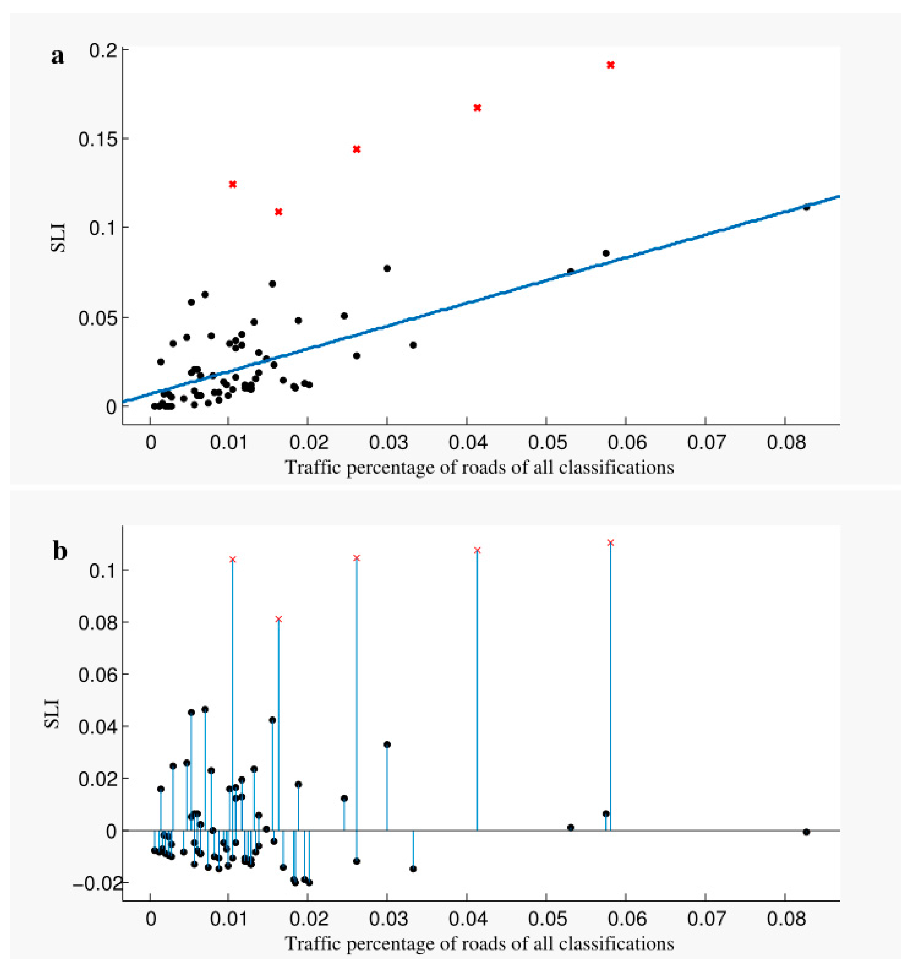
4.2. Correlation Coefficients between SLI and Traffic Flows
5. Discussion
5.1. Influence of Core Area on Traffic Flow
5.2. Influence of Landscape Diversity on Traffic Flow
5.3. Influence of Flow Landscape Patterns on Traffic Flow
5.4. The Purpose of the SLI Value
6. Conclusions
- (1)
- Source-sink landscape theory can be applied to the behavior processes of urban commuter traffic. However, the processes that are involved in commuter traffic are more consistent with an additive model than with the Location-Weighted Landscape Index (LWLI), unlike the process of accumulation of nonpoint source pollutants in natural landscapes, which can be measured by the LWLI. An additive model can better represent the relationship between the source-sink landscape pattern and commuter traffic flow.
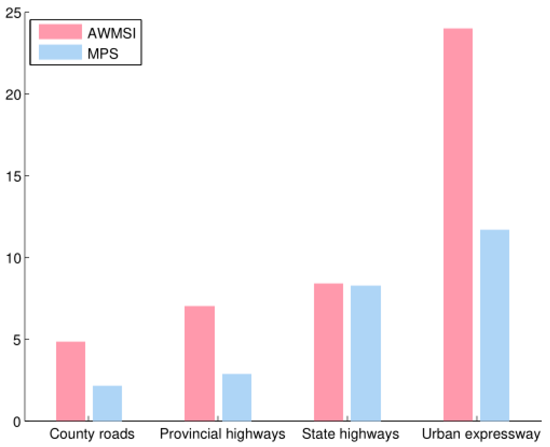
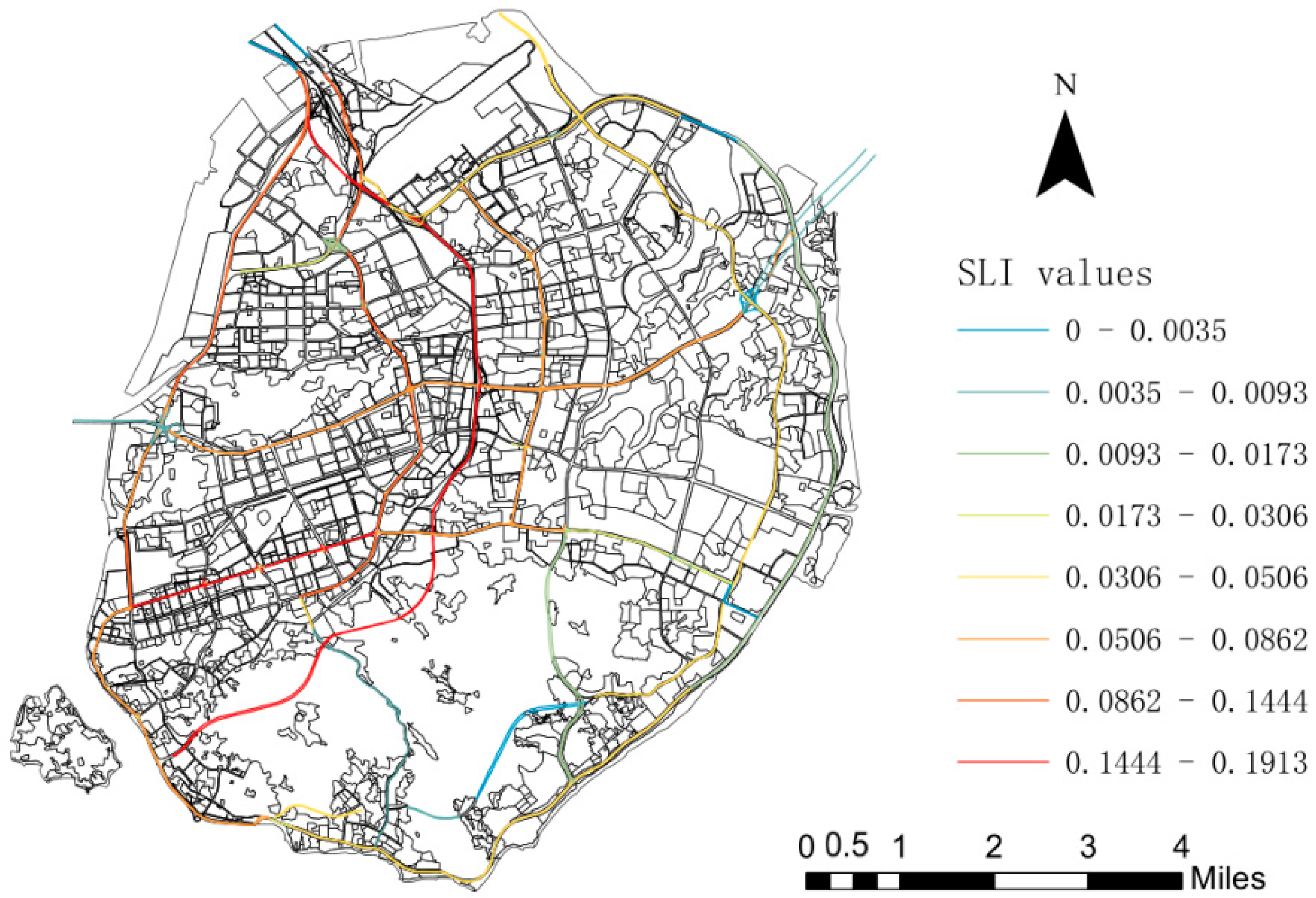
- (2)
- Different roads have different SLI values, and higher values of SLI indicate that the source-sink landscape had greater influence on traffic flow on that road. The correlation coefficient can be used to confirm these results. In this study, the SLI values of the arterial roads in Xiamen Island are highest for the urban expressway, followed by the state highways, the provincial highways, and the county roads. This indicates that the source-sink landscape patterns that are surrounding the urban expressway are most attractive to traffic flow. Commuting vehicles are more dependent on the urban expressway than on any other road.
- (3)
- Through correlation analysis, researchers can verify that there is a relationship between SLI values and traffic flows in different areas. This method allows for researchers to perform detailed analyses; for example, traditional landscape pattern indexes can be employed to find the reasons for differences in SLI values or to identify the factors that cause differences in the correlation coefficients between SLI and traffic flows. Source-sink landscape theory can contribute new ideas for the study of the relationships between urban landscape patterns and traffic.
- (4)
- This method is not designed for any specific road type; it is a method for evaluating the influence of the landscapes surrounding any road. A single SLI value is not of practical use; it must be used for comparison with different regions or time points. For example, planners can calculate and compare the SLI values in a newly developing district and in a completed area to predict commuting times, in order to determine whether there might be congestion in the new district, and to further aid in landscape planning.
Acknowledgments
Author Contributions
Conflicts of Interest
References
- Pulliam, H.R. Sources, sinks, and population regulation. Am. Nat. 1988, 132, 652–661. [Google Scholar] [CrossRef]
- Hansen, A.; Liu, J.; Hill, V.; Morzillo, A.T.; Wiens, J.A. Contribution of source-sink theory to protected area science. In Sources Sinks & Sustainability; Cambridge University Press: Cambridge, UK, 2011; pp. 339–360. [Google Scholar]
- Ludford, A.; Cole, V.J.; Porri, F.; Mcquaid, C.D.; Nakin, M.D.V.; Erlandsson, J. Testing source-sink theory: The spill-over of mussel recruits beyond marine protected areas. Landsc. Ecol. 2012, 27, 859–868. [Google Scholar] [CrossRef]
- Chen, L.; Fu, B.; Zhao, W. Source-sink landscape theory and its ecological significance. Front Acta Ecol. Sin. 2006, 26, 1444–1449. [Google Scholar] [CrossRef]
- Chen, L.; Fu, B.; Xu, J.; Gong, J. Location-weighted landscape contrast index: A scale independent approach for landscape pattern evaluation based on source-sink ecological processes. Acta Ecol. Sin. 2003, 23, 2406–2413. [Google Scholar] [CrossRef]
- Chen, L. Source-Sink Landscape Pattern Analysis and Its Applications, 1st ed.; China Science Publishing & Media Ltd.: Beijing, China, 2016; pp. 15–25. ISBN 9787030467621. [Google Scholar]
- Basnyat, P.; Teeter, L.D.; Flynn, K.M.; Lockaby, B.G. Relationships between Landscape Characteristics and Nonpoint Source Pollution Inputs to Coastal Estuaries. Environ. Manag. 1999, 23, 539–549. [Google Scholar] [CrossRef]
- Gustafson, E.J. Quantifying landscape spatial pattern: What is the state of the art? Ecosystems 1998, 1, 143–156. [Google Scholar] [CrossRef]
- Wu, J. Paradigm shift in ecology: An overview. Acta Ecol. Sin. 1996, 5, 449–459. [Google Scholar] [CrossRef]
- Lv, Y.; Chen, L.; Fu, B. Analysis of the integrating approach on landscape pattern and ecological processes. Prog. Geogr. 2007, 26, 1–10. [Google Scholar] [CrossRef]
- Jing, Y.; Zhang, S.; Li, Y. Landscape pattern and SHDI spatial structure characteristics of rural urban fringe: A case study in Jingyue development zone in Changchun city. Resour. Sci. 2007, 29, 43–49. [Google Scholar] [CrossRef]
- Chen, A.; Zhao, X.; Yao, L.; Chen, L. Application of a new integrated landscape index to predict potential urban heat islands. Ecol. Indic. 2016, 69, 828–835. [Google Scholar] [CrossRef]
- Sun, R.; Chen, L.; Wang, W.; Wang, Z. Correlating landscape pattern with total nitrogen concentration using a location-weighted sink-source landscape index in the Haihe river basin, China. Environ. Sci. 2012, 33, 1784–1788. [Google Scholar] [CrossRef]
- Li, H.; Wei, W.; Chen, J.; Li, X.; Zhang, B. Research on soil erosion based on location-weighted landscape index (LWLI) in Guanchuanhe river basin, Dingxi, Gansu province. Acta Ecol. Sin. 2013, 33, 4460–4467. [Google Scholar] [CrossRef]
- Jiang, M.; Chen, H.; Chen, Q. A method to analyze “source–sink” structure of non-point source pollution based on remote sensing technology. Environ. Pollut. 2013, 182, 135–140. [Google Scholar] [CrossRef] [PubMed]
- Li, Y. A study on the relationship between urban transportation system and urban land use structure. Trop. Geogr. 1998, 18, 307–310. [Google Scholar] [CrossRef]
- Zhou, J.; Xiao, R.; Sun, X. Relationships between settlement morphology transition and residents commuting energy consumption. Chin. J. Appl. Ecol. 2013, 24, 1977–1984. [Google Scholar] [CrossRef]
- Mao, J.; Yan, X. Study on mutual mechanism between urban transport system and urban space pattern: A case study of Guangzhou. City Plan. Rev. 2005, 29, 45–49. [Google Scholar] [CrossRef]
- Huang, N.; Lin, T.; Zhang, W.; Cao, Y. Gradient analysis and comparison of landscape pattern along different expansion axes of Tong’an district in Xiamen city. Prog. Geogr. 2009, 28, 767–774. [Google Scholar]
- Chen, T. Commuters Travel Behavior Characteristics and Analysis Method. Ph.D. Thesis, Beijing Jiaotong University, Beijing, China, 2007. [Google Scholar]
- Wang, J.; Lin, T.; Zhang, G. Spatiotemporal simulation of urban settlement morphology: A case study of Xiamen Island. Acta Ecol. Sin. 2017, 37, 2954–2969. [Google Scholar] [CrossRef]
- Ding, M. Build harmonious development of bay city’s integrative transportation system—Xiamen’s urban transportation development strategy planning. Fujian Archit. Constr. 2008, 122, 96, 115–117. [Google Scholar]
- Zhao, C.; Feng, S. Exploration about urban traffic patterns based on the multi-center spatial structure—Illustrated by the case of Xiamen. J. Qingdao Univ. Technol. 2016, 37, 53–59, 90. [Google Scholar] [CrossRef]
- Edwards, P.; Barra, T.D.L. Integrated land use and transport modelling: Decision chains and hierarchies. J. R. Stat. Soc. 1989, 42, 191. [Google Scholar] [CrossRef]
- De la Barra, T.; Perez, B.; Vera, N. TRANUS-J: Putting large models into small computers. Environ. Plan. B Plan. Des. 1984, 11, 87–101. [Google Scholar] [CrossRef]
- Zhou, J.; Lin, J.; Cui, S.; Qiu, Q.; Zhao, Q. Exploring the relationship between urban transportation energy; consumption and transition of settlement morphology: A case study on Xiamen Island, China. Habitat Int. 2013, 37, 70–79. [Google Scholar] [CrossRef]
- Qiu, Q. Simulation of Residential Commuting Travel and Evaluation of Carbon Emission under Transformation of Urban Settlement Morphology. Ph.D. Thesis, Graduate University of Chinese Academy of Sciences, Beijing, China, 2011. [Google Scholar]
- Zhang, Y.; Feng, X.; Du, J.; Gu, G. Study on extraction of urban green space from IKONOS remote sensing images. Geogr. Res. 2004, 23, 274–280. [Google Scholar] [CrossRef]
- Xie, J.; Li, Y. The extraction of building distribution information of different heights in a city from the shadows in a IKONOS image. Remote Sens. Land Resour. 2004, 16, 4–6. [Google Scholar] [CrossRef]
- Shu, S.; Yang, M. Hyperspectral image classification method based on watershed segmentation and sparse representation. Comput. Sci. 2016, 43, 89–94. [Google Scholar] [CrossRef]
- Modelistica. TRANUS: Integrated Land Use and Transport Modeling System, Modelistica Company: Caracas, Venezuela; Mexico, 2007.
- Chen, L.; Tian, H.; Fu, B.; Zhao, X. Development of a new index for integrating landscape patterns with ecological processes at watershed scale. Chin. Geogr. Sci. 2009, 19, 37–45. [Google Scholar] [CrossRef]
- Dai, Q.; Liu, G.; Jiang, X.; Liu, M.; Wang, Y. An evaluation on sustainable development of eco-economic system in small watershed in hilly area of northeast China. Acta Geogr. Sin. 2005, 60, 209–218. [Google Scholar]
- Huang, N.; Lin, T.; Chen, X. Analysis and comparison of landscape patterns in the surroundings of different traffic lines—Xiamen Island as an example. Yunnan Geogr. Environ. Res. 2009, 21, 42–46, 51. [Google Scholar] [CrossRef]
- Yang, Y. Urban fringe extraction and its change monitoring using multi-temporal tm image. Remote Sens. Inf. 2009, 3, 49–53. [Google Scholar] [CrossRef]
- Huang, S.; Chen, Y.; Zhang, R.; Wu, W.; Wei, C. Spatial correlation analysis of land fragmentation and agriculture development based on landscape indexes. Agric. Res. Arid Areas 2015, 3, 238–244. [Google Scholar] [CrossRef]
- Li, H.; Li, S.; Lv, T.; Liu, C. Evaluation of farmland fragmentation due to the impact of land consolidation based on the view of landscape pattern. Resour. Environ. Yangtze Basin 2017, 26, 67–73. [Google Scholar] [CrossRef]
- Yang, S. Effect of Road on Landscape Structure in Shenzhen City. Master’s Thesis, Beijing University, Beijing, China, 2012. [Google Scholar]
- Zupanovic, D.; Grgurevic, I.; Filipcic, T. Importance of collecting and analyzing data on traffic flow load in urban environments. In Proceedings of the 30th International Conference on Information Technology Interfaces, Dubrovnik, Croatia, 23–26 June 2008; pp. 809–814. [Google Scholar] [CrossRef]
- Oh, S.D.; Kim, Y.J.; Hong, J.S. Urban traffic flow prediction system using a multifactor pattern recognition model. IEEE Trans. Intell. Transp. Syst. 2015, 16, 2744–2755. [Google Scholar] [CrossRef]
- Liang, H. Diverging traffic flows and design patterns for urban corridors. Urban Transp. China 2009, 7, 78–84. [Google Scholar] [CrossRef]


| Road Classification | SLI Correlation Coefficient | Significance (Two-Tailed Test) | LWLI Correlation Coefficient | Significance (Two-Tailed Test) |
|---|---|---|---|---|
| County road | 0.710 ** | 0 | 0.001 | 0.994 |
| Provincial highway | 0.731 ** | 0.001 | −0.130 | 0.608 |
| State highway | 0.891 * | 0.0417 | 0.017 | 0.978 |
| Total | 0.684 ** | 0 | −0.024 | 0.843 |
| Land Usage Type | Correlation Coefficient |
|---|---|
| Urban residential land | 0.739 |
| Residential land in urban village | 0.480 |
| Educational land | 0.117 |
| Industrial and mining land | 0.582 |
| Construction site | −0.001 |
| Commercial and service land | 0.541 |
| Mixed commercial and residential land | 0.516 |
| Land Usage Type | Road Classification | Core Area (m2) | Percentage of Core Area (%) | Contribution of Core Area |
|---|---|---|---|---|
| Urban residential land | Urban expressway | 673.2219 | 0.5067 | 0.0583 |
| State highway | 519.6150 | 0.4078 | 0.0276 | |
| Provincial highway | 3239.9974 | 0.4149 | 0.0110 | |
| County road | 5385.2851 | 0.3561 | 0.0053 | |
| Urban village land | Urban expressway | 115.2985 | 0.0868 | 0.0100 |
| State highway | 114.5621 | 0.0899 | 0.0061 | |
| Provincial highway | 890.3992 | 0.1140 | 0.0030 | |
| County road | 2155.4179 | 0.1425 | 0.0021 | |
| Industrial and mining land | Urban expressway | 286.9834 | 0.2160 | 0.1912 |
| State highway | 86.8192 | 0.0681 | 0.0238 | |
| Provincial highway | 932.5871 | 0.1194 | 0.0219 | |
| County road | 2500.7271 | 0.1654 | 0.0242 | |
| Commercial and service land | Urban expressway | 143.6290 | 0.1081 | 0.0957 |
| State highway | 99.0594 | 0.0777 | 0.0271 | |
| Provincial highway | 824.2738 | 0.1056 | 0.0193 | |
| County road | 1315.4769 | 0.0870 | 0.0127 | |
| Mixed commercial and residential land | Urban expressway | 41.1475 | 0.0310 | 0.0036 |
| State highway | 60.2074 | 0.0472 | 0.0032 | |
| Provincial highway | 342.7641 | 0.0439 | 0.0012 | |
| County road | 360.0863 | 0.0238 | 0.0004 |
© 2017 by the authors. Licensee MDPI, Basel, Switzerland. This article is an open access article distributed under the terms and conditions of the Creative Commons Attribution (CC BY) license (http://creativecommons.org/licenses/by/4.0/).
Share and Cite
Wu, T.; Tang, L.; Chen, H.; Wang, Z.; Qiu, Q. Application of Source-Sink Landscape Influence Values to Commuter Traffic: A Case Study of Xiamen Island. Sustainability 2017, 9, 2366. https://doi.org/10.3390/su9122366
Wu T, Tang L, Chen H, Wang Z, Qiu Q. Application of Source-Sink Landscape Influence Values to Commuter Traffic: A Case Study of Xiamen Island. Sustainability. 2017; 9(12):2366. https://doi.org/10.3390/su9122366
Chicago/Turabian StyleWu, Tong, Lina Tang, Huaxiang Chen, Ziyan Wang, and Quanyi Qiu. 2017. "Application of Source-Sink Landscape Influence Values to Commuter Traffic: A Case Study of Xiamen Island" Sustainability 9, no. 12: 2366. https://doi.org/10.3390/su9122366
APA StyleWu, T., Tang, L., Chen, H., Wang, Z., & Qiu, Q. (2017). Application of Source-Sink Landscape Influence Values to Commuter Traffic: A Case Study of Xiamen Island. Sustainability, 9(12), 2366. https://doi.org/10.3390/su9122366