1. Introduction
Due to the exacerbating concerns on the global environment, the concept of sustainable development has been widely accepted by industry and academy, thereby contributing to the continuously prosperous research on sustainable supply chain management (SSCM) as well as green supply chain management (GSCM) [
1,
2]. GSCM pressurizes supply chain members into integrating environmental thoughts into supply chain management including product design, material souring and selection, manufacturing processes, delivery of the final product as well as end of life management of the product after its useful life [
3]. Sustainability can be a valuable, rare, inimitable and non-substitutable resource that becomes a source of competitive advantage [
4]. The application of GSCM can improve the environmental and economic performance of organizations, as well as enable enterprises to obtain competitive advantage, which encourages organizations to be continually sustainable [
5,
6]. GSCM has emerged as an important organizational philosophy to achieve corporate profit and market share objectives [
7].
Green products play a significant role in the development of GSCM with regard to the decision making process [
8]. Under environmental pressure, governments have placed multiple enforcement and policies to abate pollution, and these top-down policies contribute to external factors for the company to go green consequently [
9]. On the other hand, pressure of growing green demand also exerts bottom-up driving forces to firms. Green innovation is regarded as a survival need for firms to keep competitiveness [
10]. Therefore, an increasing of manufacturers engages in the R&D, production and sale of green products. Driessen conducts case studies in chemical and food industries and reveals that both giant manufacturers and SMEs produce green products [
11]. However, there is anecdotal evidence of the market success and/or failure of green product regardless of giant manufacturers or SMEs [
12].
Literature has extensively examined factors contributing to market performance of green products. Pujari suggests market orientation or market focus is one of the key factors [
13]. Driessen reveals that product greenness has been examined as a pivotal role in marketing of green product [
11]. Researches related to green management have quantitatively examined the product greenness strategy. Li et al. investigate the greenness level and pricing problems in a competitive dual channel green supply chain [
8]. Zhu and He study the green product design issues in supply chains where manufacturer produces development-intensive product or marginal-cost intensive product [
14]. Yang and Xiao analyze the pricing and green level decisions of a green supply chain with government interventions [
15]. However, few researches study the influences of manufacturers’ market power on the greenness and pricing strategies of green products.
Motivated by the above facts, the paper explores the green supply chain with duopoly manufacturers considering different manufacturers’ market power. One manufacturer produces green product, another produces traditional product, and both green and traditional product are sold to end customers through a common retailer. The manufacturers and retailer play a manufacturer-leader Stackelberg game, while two manufacturers play three subgame: (1) green manufacturer oriented Stackelberg game (giant green manufacturer and traditional SME); (2) traditional manufacturer oriented Stackelberg game (giant traditional manufacturer and green SME); and (3) Bertrand game of two manufacturers where two manufacturer have equal market power. Furthermore, previous researches have suggested the efficiencies of first-mover advantage [
16], as well as green competitive advantage [
14], in the green supply chain. However, to the best of authors’ knowledge, few researches were found to investigate the relation of green competitiveness and first-mover advantage in the domain of green supply chain management. Thus, we want to address following questions by establishing and solving models in three sceneries: (1) How manufacturers’ market power influences the pricing policies and green strategies of supply chain members in a green supply chain? (2) What conditions do first-mover advantage and green competitive advantage be effective simultaneously?
The main contribution of the paper is threefold. First, the paper investigates the influences of manufacturers’ different market power on members’ pricing policies and green strategies in a green supply chain. Second, we find that manufacturers’ optimal decisions and total profit in the three models are consistent, but retailer’s optimal decisions and total profit in the three models are inconsistent. Third, we discover that the green competitive advantage is more effective than first-mover advantage while first-mover advantage does not always be effective in the duopoly green supply chain. Specially, traditional manufacturer always prefers to be the follower competing with the green manufacturer, while whether green manufacturer would like to be the leader depends on the level of consumer’s environmental awareness and the value of greening cost effector.
The reminder of this paper is organized as follows.
Section 2 provides the problem description and notations. We establish three pricing game models and obtain the corresponding equilibrium solutions in
Section 3. Sensitivity analysis of the main parameters on equilibrium solutions are given in
Section 4.
Section 5 conducts a numerical example to compare the optimal pricing strategies, greenness degree and maximal profits under three members’ different market power.
Section 6 provides concluding remarks.
2. Model Formulation
The paper considers a two-echelon supply chain with two manufacturers and a common retailer in a green market where consumers are environmental aware. The manufacturer 1 (M1) produces a green product (Product 1) and wholesales it to the retailer at wholesale price
w1 with unit production cost
c1. The green product is featured with greenness degree
θg and traditional product is featured with greenness degree
θt. Similar to Madani’s work [
5], we set the greenness degree of traditional product as benchmark and assume
θt = 0. Moreover, we assume the greenness degree of green product is
θ, thus,
θg =
θ.
θ in the paper is assumed to reflect the general impact from different green attributes of the green product [
14]. The manufacturer 2 (M2) produces a traditional product (Product 2) and wholesales it to the retailer at wholesale price
w2 with unit cost
c2, then the retailer sells the product 1 and 2 to the end consumers at retail price
p1 and
p2 respectively.
To investigate the influences of manufacturers’ market power on the pricing policies and green strategies of supply chain members in a green supply chain, we assume that there are giant manufacturers and SMEs in the green market. Therefore, there are four combinations of manufacturer’ market power and types of product: Combination (1) giant green manufacturer and traditional SMEs; Combination (2) giant traditional manufacturer and green SMEs; Combination (3) giant green manufacturer and giant traditional manufacturer; and Combination (4) green SMEs and traditional SMEs. Corresponding to the four combinations, we formulate three game scenarios: Scenario (1) M1-leader Stackelberg game (Combination (1)); Scenario (2) M2-leader Stackelberg game (Combination (2)); and Scenario (3) Bertrand game (Combinations (3) and (4)). The timing of moves of the manufacturers in the three scenarios are as follows:
- (I)
M1-M2 Bertrand game: The two manufacturers move simultaneously. Specifically, manufacturer 1 announces the marginal profit mM1 and green degree θ, and manufacturer 2 sets the marginal profit mM2, simultaneously.
- (II)
M1-oriented Stackelberg game: The two manufacturers move sequentially. Manufacturer 1 acts as the leader and manufacturer 2 acts as the follower. Specifically, manufacturer 1 decides the marginal profit mM1 and green degree θ first, and then manufacturer 2 sets its marginal profit mM2.
- (III)
M2-oriented Stackelberg game: The two manufacturers move sequentially. Manufacturer 2 acts as the leader and manufacturer 1 acts as the follower. Specifically, manufacturer 2 sets its marginal profit mM2 first, and then manufacturer 1 decides its marginal profit mM1 and green degree θ.
Based on the facts that consumers are willing to pay higher prices for more eco-friendly products [
17,
18], we assume greenness degree is a demand enhancement factor of demand. We assume that the market demand functions are linear with the retail prices and greenness degree of green product, and retail price of traditional product [
14,
19]. The demand functions of green product and traditional product are as follows, respectively
Parameter α denotes the total market demand, β represents the self-price sensitivity. γ is the cross-price sensitivity coefficient, and β > γ > 0, which indicates that the change of pi has more significant impact on demand of product i than the change of the sale price of its rival product (i = 1, 2). δ denotes the level of consumer’s environmental awareness. When the consumer’s environmental awareness is at a relatively high level, the influence of greenness degree on product demand is more remarkable. The higher δ is, the greater demand of green product is. Thus, δ is also the expansion effectiveness coefficient of the greenness degree per unit of green product. The constraint β > δ > 0 means that the retail price is the dominant factor on product demand instead of greenness degree.
To engage in green product production, only the green product manufacturer (Manufacturer 1) has to invest extra capital to employ green technologies based on the original production process. We assume that the greening improvement in the product does not affect the manufacturer’s traditional marginal costs of production [
5,
8]. It is common knowledge that firms make initial changes in products and process easily, while the subsequent improvement being more difficult [
20]. Thus, we assume that the cost of greening is a quadratic function of green degree
c(
θ) =
hθ2 [
18].
represents the greening investment coefficient, a larger
means the improvement of green degree requires greater investment and that it is harder to achieve green innovation when the greenness degree reaches a relatively high level. To avoid trivial things, we assume
.
Denote
and
as the marginal profit of manufacturer 1 and 2 from producing a unit product. Then the wholesale price comprises the manufacturer’s marginal profit and unit production cost, namely,
and
. Denote
and
as the marginal profit of retailer for selling unit product 1 and 2. Then the product sale price consists of the retailer’s marginal profit and wholesale price. We also assume that the retailer’s sale efforts of those two products are consistent. Thus, we can have
and
. Denote
,
, and
are the profit of manufacturer 1, manufacturer 2 and retailer respectively. Based on the above assumptions, the players’ profit functions are as follows:
3. Model Solution
In this section, the relationships between two manufacturers and the retailer are modeled as a sequential non-cooperative game, where the two manufacturers are the leaders while the retailer is the follower. The timing of moves are as follows: (1) the two manufacturers determine decision variables at first; (2) The retailer sets the retail price based on the manufacturers’ decisions. Similar to Zhao’s [
21], we mainly consider the situations where the two manufacturers implement the three game scenarios introduced in
Section 2.
After observing the two manufacturers’ decisions, the retailer determines the retail prices of the two products to maximize its profit. By backward induction, we first derive the retailer’s response functions.
Proposition 1. Given earlier decisions mM1 and θ made by the manufacturer 1, and mM2 made by the manufacturer 2, the retailer’s response functions are as follows.
The proofs of Proposition 1 and other propositions are enclosed in
Appendix A. From the retailer’s response functions, the results of Corollary 1 can be obtained.
Corollary 1. - (1)
, ;
- (2)
;
- (3)
.
With the increasing greenness degree of product 1, the retailer’s marginal profit from selling product 1 increases while the marginal profit from selling product 2 decreases. When the greenness degree of green product improved consistently, the retailer should increase the order quantity of green product and decrease the order quantity of traditional product. In addition, it reveals the efficiency of first-mover advantage that retailer’s marginal profits from selling product 1 and 2 decrease when the manufacturer 1’s and 2’s marginal profits increase.
3.1. Bertrand Game
In this setting, two manufacturers play Bertrand game. By backward induction, after knowing the retailer’s response functions, the two manufacturers make optimal decisions to maximize their own profits simultaneously. The M1-M2 Bertrand game model can be formulated as
The following proposition gives the two manufacturers’ optimal decisions.
Proposition 2. In the Bertrand game, the manufacturer 1’s optimal marginal profit and greenness degree ,
and the manufacturer 2’s optimal marginal profit can be given as Substituting Equations (10)–(12) into Equations (8) and (9), we can obtain the retailer’s optimal marginal profits in the Bertrand model.
3.2. M1-Oriented Stackelberg
In this setting, two manufacturers play Stackelberg game and move sequentially. The manufacturer 1 acts as the leader and decides the marginal profit
and greenness degree
to maximize its profit at first, and manufacturer 2 acts as the follower and sets its marginal profit
to maximize its profit later. The M1-oriented Stackelberg game model can be formulated as
Proposition 3. Given the decisions and made by the manufacturer 1, the manufacturer 2’s response function is as follow Corollary 2. , .
Manufacturer 2’s marginal profit will be increased if manufacturer 1’s marginal profit increases, which is different from the implication of Corollary 1. Furthermore, manufacturer 2’s marginal profit will be decreased if greenness degree of product 1 increases. The magnitude of the reduction depends on the level of consumer’s environmental awareness. Thus, in the M1-oriented Stackelberg subgame, manufacturer 1 benefits from green competitive advantage while manufacturer 2 benefits from the second-mover advantage as being the follower.
Proposition 4. In the M1-oriented Stackelberg model, the manufacturer 1’s optimal marginal profit and greenness degree ,
the manufacturer 2’s optimal marginal profit and the retailer’s optimal marginal profits and can be given as 3.3. M2-Oriented Stackelberg
In this setting, two manufacturers play Stackelberg game and move sequentially. The manufacturer 2 acts as the leader and decides the marginal profit
to maximize its profit at first, and then the manufacturer 1 acts as the follower and sets its marginal profit
and greenness degree
to maximize its profit later. The M1-oriented Stackelberg game model can be formulated as
Proposition 5. Given the decision made by the manufacturer 2, the manufacturer 1’s response functions are as follows Corollary 3. , .
Manufacturer 1’s marginal profit and the greenness degree of product 1 will increase with the increasing of manufacturer 2’s marginal profit. In the M2-M1 Stackelberg subgame, manufacturer 1 benefits from second-mover advantage as being the follower.
Proposition 6. In the M2-oriented Stackelberg model, the manufacturer 2’s optimal marginal profit ,
the manufacturer 1’s optimal marginal profit and greenness degree ,
and the retailer’s optimal marginal profits and can be given as 4. Sensitivity Analysis
In this section, we conduct the sensitivity analysis of the equilibrium decisions and the maximum profits with respect to parameters and . Properties 1–3 summarize the sensitivities with respect to the equilibrium decisions. Properties 4–6 summarize the sensitivities with respect to the players’ profits.
Property 1. - (1)
In the three sceneries, the sensitivities of the optimal decisions with respect to the parameter are given as , , , and ;
- (2)
Denotes is the total marginal profit from selling a unit green product and a unit traditional product, namely, . The sensitivities of the retailer’s optimal marginal profit with the parameter are given as:
- (i)
In the settings of Bertrand, ;
- (ii)
In the setting of M1-oriented Stackelberg game, ;
- (iii)
In the setting of M2-oriented Stackelberg game, .
The proof of Property 1 and other remaining properties appears in
Appendix B.
Property 1 investigates that the increase of greening cost effector diminishes green participators’ marginal profits. The manufacturer 1’s marginal profit and retailer’s marginal profit from selling green product decline while the value of greening cost effector rises. A great greening cost not only discourages the green manufacturer from devoting to green innovations but also depresses the retailer’s willingness of selling green products. Further, with the increase of greening cost effector, the retailer’s marginal profit from selling green product goes down while the marginal profit from selling traditional product goes up. What’ more, the retailer’s total marginal profit drops in the M2-oriented Stackelberg game, increases in the M1 oriented Stackelberg game and keeps the same in the Bertrand game. Thus, the retailer should raise the order quantity of traditional product and decrease the order quantity of green product, especially when traditional manufacturer acts as the leader.
Property 2. The sensitivities of the optimal decisions with parameter are obtained as
- (1)
, , , , ;
- (2)
The sensitivities of the optimal marginal profit with are given as follows:
- (i)
In the setting of Bertrand model, ;
- (ii)
In the setting of M1-oriented Stackelberg and M2-oriented Stackelberg models, .
The manufacturer 1’s marginal profits and retailer’s marginal profit from selling green product increase as the level of consumer’s environmental awareness rises. However, the manufacturer 2’s marginal profit and the retailer’s marginal profit from selling gray product go down if rises. Thus, the green innovation participators, both the green manufacturer and retailer, should take measures to improve the level of consumer’s environmental awareness. Meanwhile, the retailer’s total marginal profits are positive with the consumers’ environmental awareness when the manufacturers’ market power are different. Specially, the retailer’s total marginal profit is constant when the consumer’s environmental awareness changes when the manufacturers have the same market power. The retailer should increase the order quantity of green product and decrease the order quantity of traditional product.
Property 3. The sensitivities of retail prices with parameter and are obtained as , , and .
The sale price of green (traditional) product is positive (negative) with the consumer’s environmental awareness but negative (positive) with the green investment effector. When the greening cost effector increase, the retailer should raise the sale price of traditional product but drop the sale price of green product. On the other hand, when the consumer’s environment awareness is improved, the retailer should drop the sale price of traditional product but raise the sale price of green product.
Property 4. The sensitivities of the manufacturer 1’s total profit with parameter and are obtained as and .
The increasing of greening cost effector would impair the green manufacturer’s total profit, on the contrary, the increasing of consumer’s environmental awareness would enlarge its total profit. Thus, the green manufacturer should take marketing activities to encourage the public noticing the environmental issues and seek the green technical breakthroughs to decrease the investment of green product research and development. Further, governments should provide suitable incentives like tax-cut or green subsidy to encourage enterprises to devote in green manufacturing.
Property 5. The sensitivities of the manufacturer 2’s total profit with parameter and are obtained as
- (1)
If , then ; otherwise ;
- (2)
If , then ; otherwise .
Only when parameters and have positive influences on the maximal demand of traditional product can the manufacturer 2 increases its maximal profit. Therefore, it is beneficial for the traditional manufacturer to take marketing activities to promote market demand, i.e., enlarging the market potential demand by advertising or establishing new sale channels.
Property 6. Denotes the retailer’s profit from product 1 as and profit from selling product 2 as . Then
- (1)
, , ;
- (2)
In the setting of M1-M2 Bertrand model, ;
- (3)
In the setting of M1-oriented Stackelberg and M2-oriented Stackelberg model, .
In the three game models, the retailer’s profit from selling green product is positive to but negative to . Furthermore, the retailer’s profit from selling traditional product is negative to .
The consumer’s environmental awareness has positive effect on retailer’s profit from product 1, but has negative impact on retailer’s profit from product 2. The green investment coefficient is negative to the retailer’s profit from product 1, but its influences on retailer’s profit from product 2 depends on the market power structure of manufacturers. Thus, when the consumer’s environmental awareness is relatively high, the retailer should raise the order quantity of green product. When the manufacturers have equal market power, it is beneficial for the retailer to seek approaches to decrease the greening cost effector. However, when the manufacturers have unequal market power, the retailer should enlarge the order quantity of traditional product to maximize its total profit.
5. Numerical Examples
In this section, we compare the players’ optimal decisions and maximum profits under three scenarios and derive more managerial implications by providing numerical examples. The values of various model parameters are listed as follows. , , , and . We take the identical values of parameters in order to separate the effects of different power structures in three decision models in each parameter.
5.1. Sensitivity Analysis of Consumer’s Environmental Awareness
This subsection explores how consumer’s environmental awareness affects the green supply chains. We set
, and the value of
varies from 0 to 4.
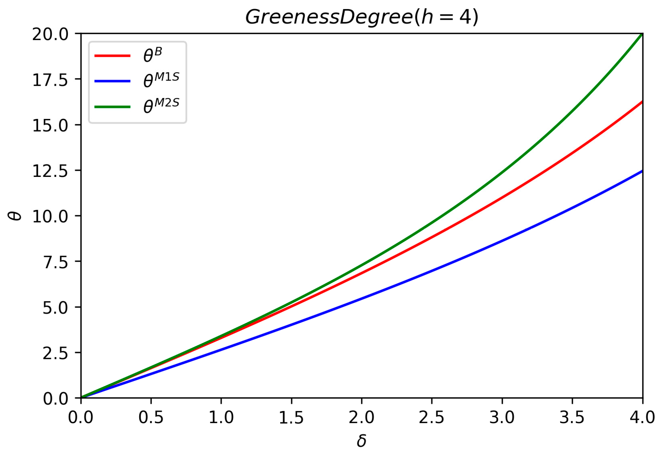
Figure 1 verifies the positive correlations between greenness degree and consumer’s environmental awareness under three sceneries. To protect environment, the government, as well as other public organization should devote to green propaganda to enhance public awareness of environmental protection. The formula
is constantly tenable for any given value of
. When the manufacturer 1 acts as the leader, he possesses double advantages, namely, the first-mover advantage and green competitive advantage. However, when the manufacturer 1 acts as the follower, he is in green competitive advantage but at a later disadvantage. Thus, his willingness of improving green degree is stronger at the setting of M2-oriented Stackelberg game compared to M1-oriented Stackelberg game. This finding implicates that the competition between manufacturers contributes to the improvement of greenness degree.
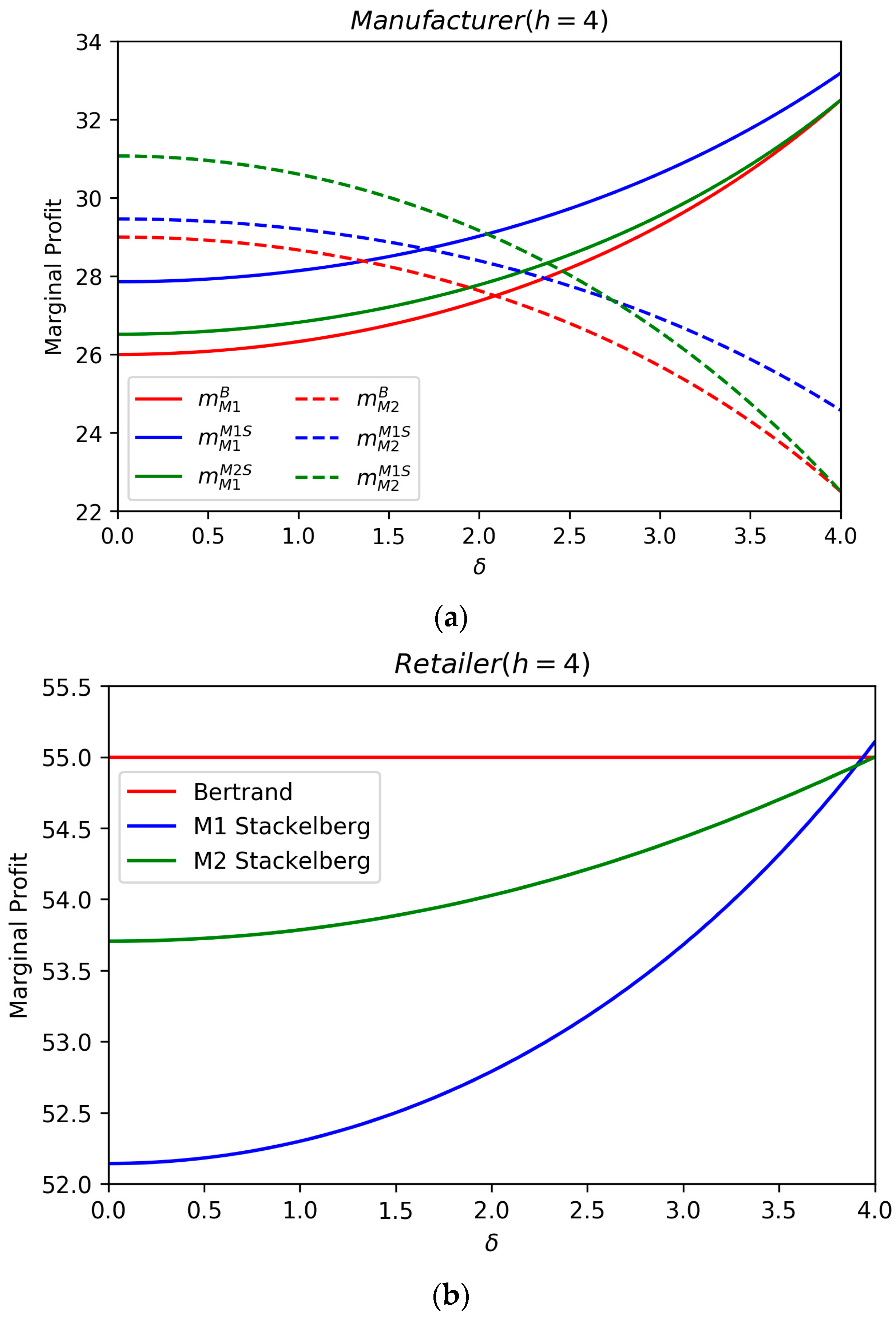
Figure 2 investigates the effect of
on players’ marginal profits under three sceneries. From
Figure 2a,
increases but
decreases as the value of
increases. Manufacturer 1 obtains greatest marginal profit in M1-oriented Stackelberg game, middle in M2-oriented Stackelberg game and least in M1-M2 Bertrand game. Furthermore, manufacturer 2 obtains the greatest marginal profit in M2-oriented Stackelberg game when the value of
is lower than a threshold, but, contrariwise, he obtains the greatest marginal profit in M1-oriented Stackelberg game when the value of
is higher than the threshold.
Figure 2b shows that the retailer gains the greatest total marginal profit in M1-M2 Bertrand model than other two models generally. Furthermore, the formula
is tenable except the situation where
is excessively large. Therefore, it is beneficial for the retailer to take actions to narrow the gap between manufacturers’ market power, but help the manufacturer 2 keeping its leader position. On the other hand, the retailer should help manufacturer 1 to accelerate the consumer’s environmental awareness.
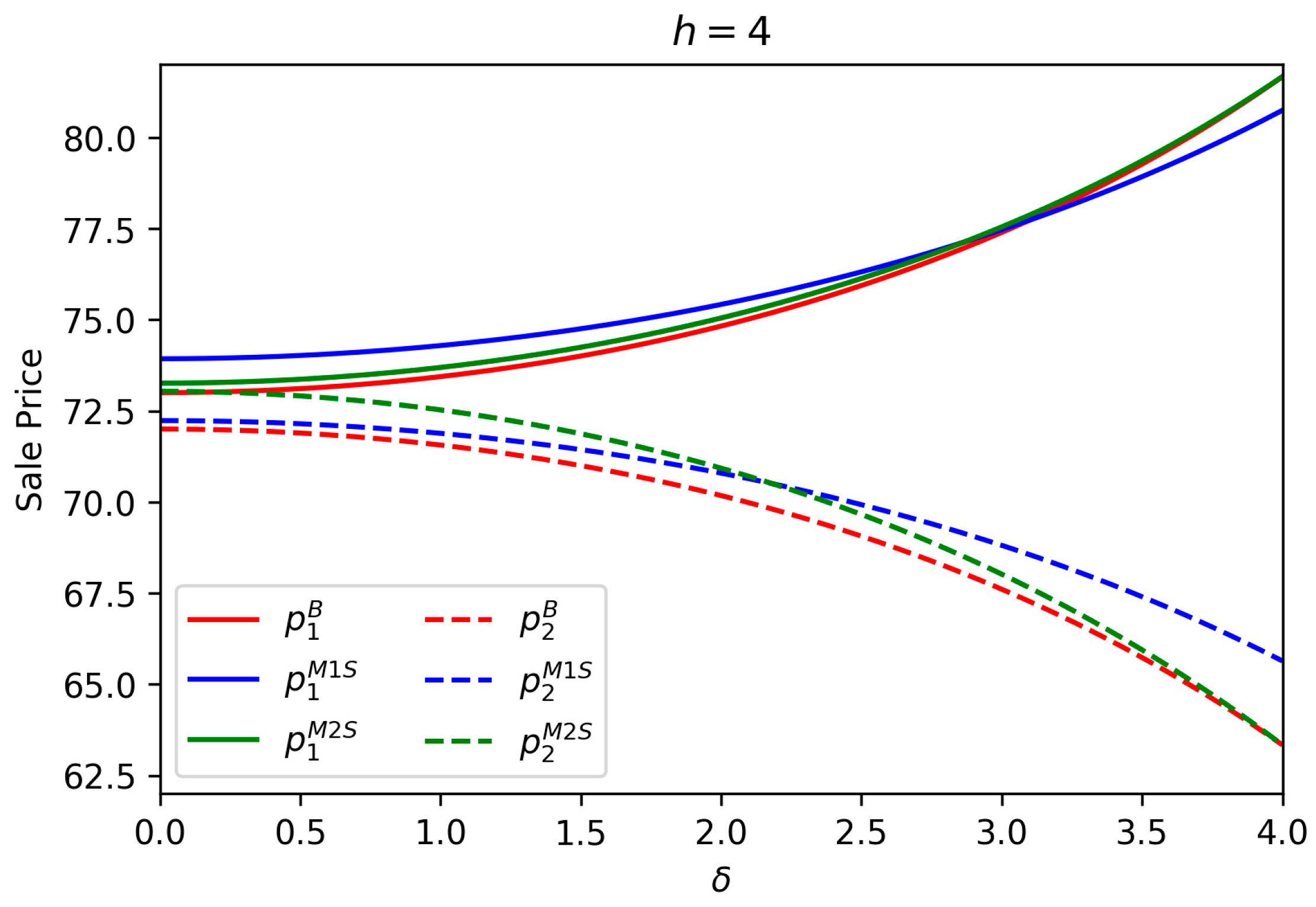
Figure 3 displays the correlations between product sale prices and parameter
.
Figure 3 shows the positive effects of
on green product sale price and the negative influence of
on traditional product sale price. For a given value of
, the sale price of green product is always higher than traditional product in each game model. Additionally, the disparity is widened with the increase of
, which is consistent to the fact that consumers with higher environmental awareness are willing to pay more to green product. It suggests that the retailer should rise the green product sale price but lower the traditional product sale price when the value of
increases.
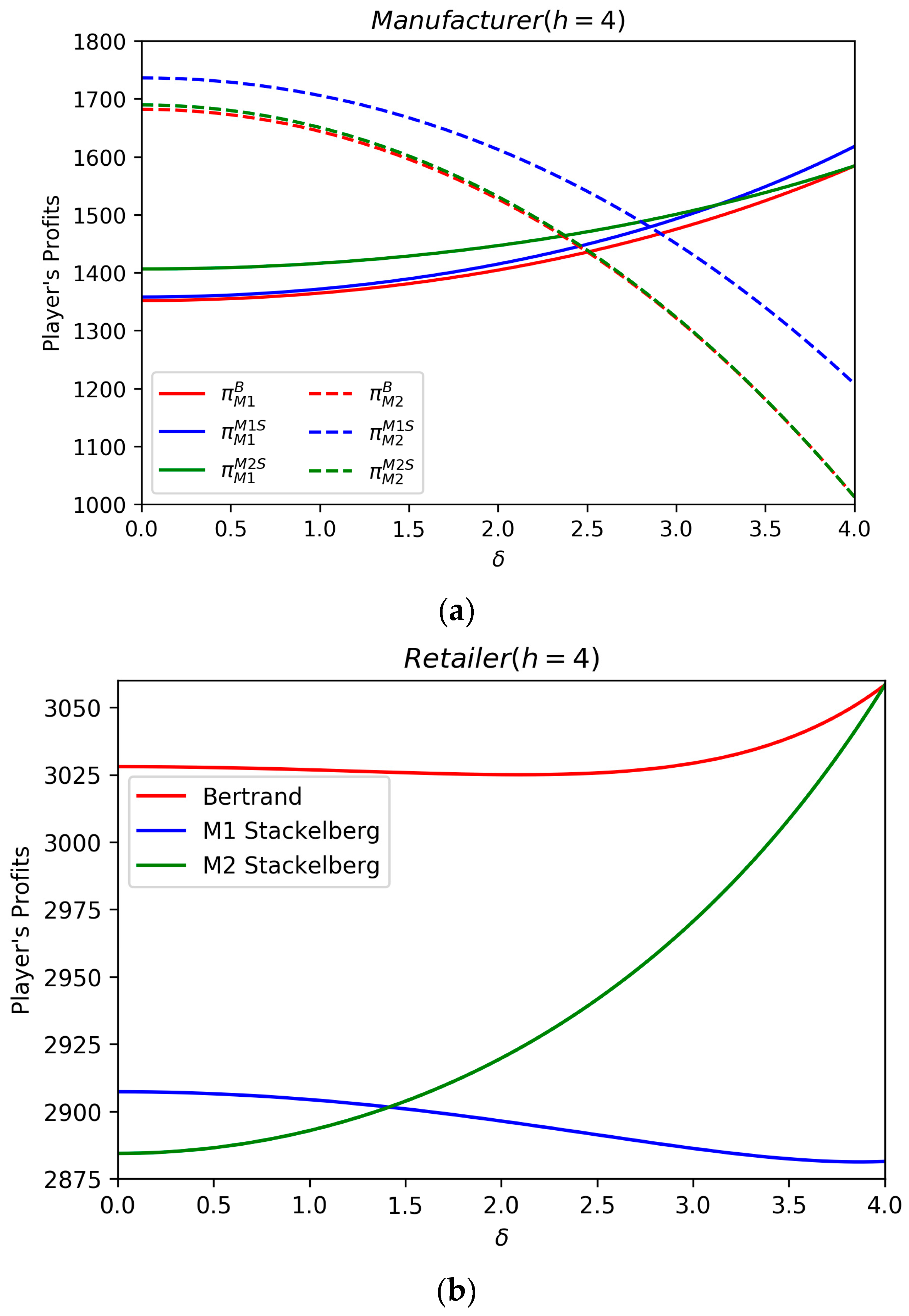
Figure 4 demonstrates the effects of
on player’s profits. We can explore the positive effects of
on manufacturer 1’s profits and the negative effects on manufacturer 2’s profits. Manufacturer 1 obtains greatest profit in M2-oriented Stackelberg game when the value of
is lower than a threshold, but gets greatest profit in M1-oriented Stackelberg game when the value of
is higher than the threshold. It reveals that only in a particular environment can the first mover advantage and green competitive advantage are effective together. Furthermore, we find that the formula
is constantly tenable for any given value of
. It is interesting to find that the optimal strategy for manufacturer 2 is to be a follower when consumers are environmentally aware. Further, it is advisable for manufacturer 1 to be the follower when the value of
is lower than a threshold, but to be the leader when the value of
is higher than the threshold.
Figure 4b shows that the retailer earns the greatest profit in M1-M2 Bertrand model. We find that the formula
is tenable when
is at a relatively low level. Further, the retailer’s profit is positive to
in M2-oriented Stackelberg model but is negative in M1-oriented Stackelberg model. From the perspective of retailer, the optimal strategy is taking actions to narrow the gap between manufacturers’ market power. The suboptimal strategy is supporting manufacturer 1 to be leader when the consumer’s environmental awareness is low, while backing manufacturer 2 to be leader when the consumer’s environmental awareness is high.
5.2. Sensitivity Analysis of Greening Cost Effector
This subsection explores how the greening cost effector affects the green supply chains. We set
, and the value of
varies from 1 to 11.
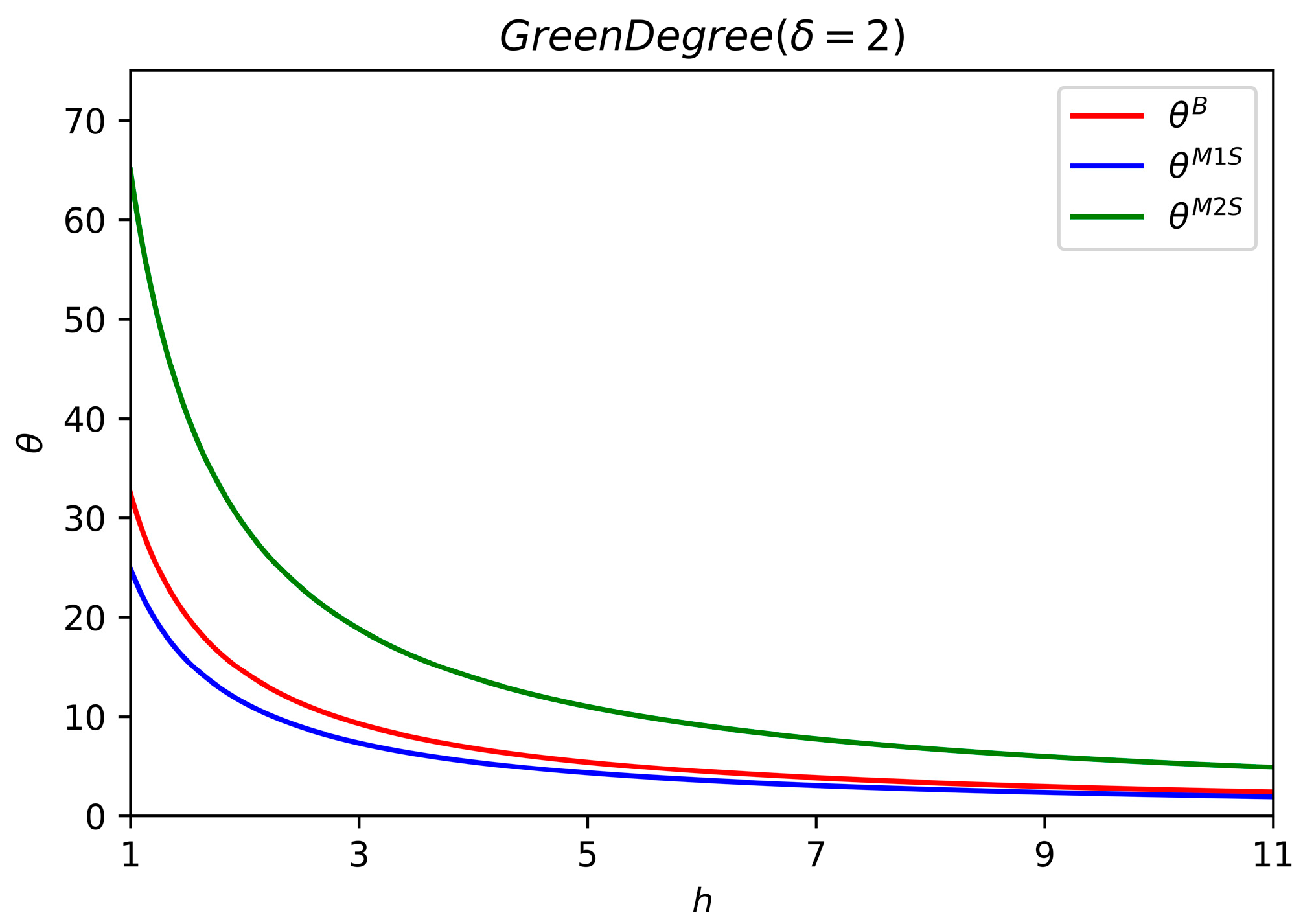
Figure 5 displays the negative effects of
on the optimal green degree of product 1. Greening cost plays a significant role in green product production and the increment of greening cost imposes a heavy burden on manufacturer 1. To support green product producer’s green innovation and protect environment, government should formulate policies to help enterprises lowering the greening cost, i.e., providing green subsidy or taxes reduction to the companies devoted to greening products. It is easy to observe that the formula
is constantly tenable for any given value of
. Similarly, the greenness degree of product is greatest when the manufacturer 1 acts as a follower.
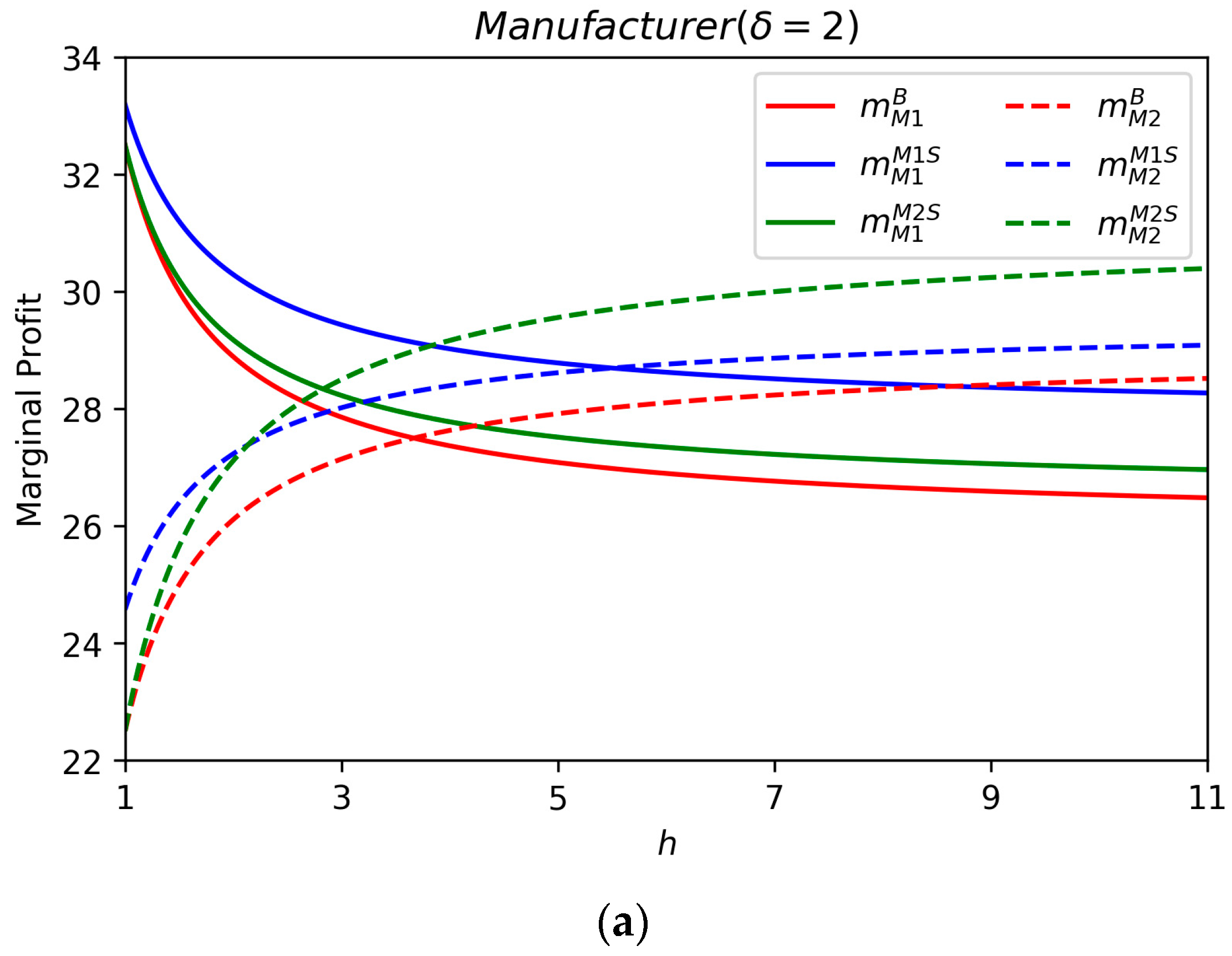
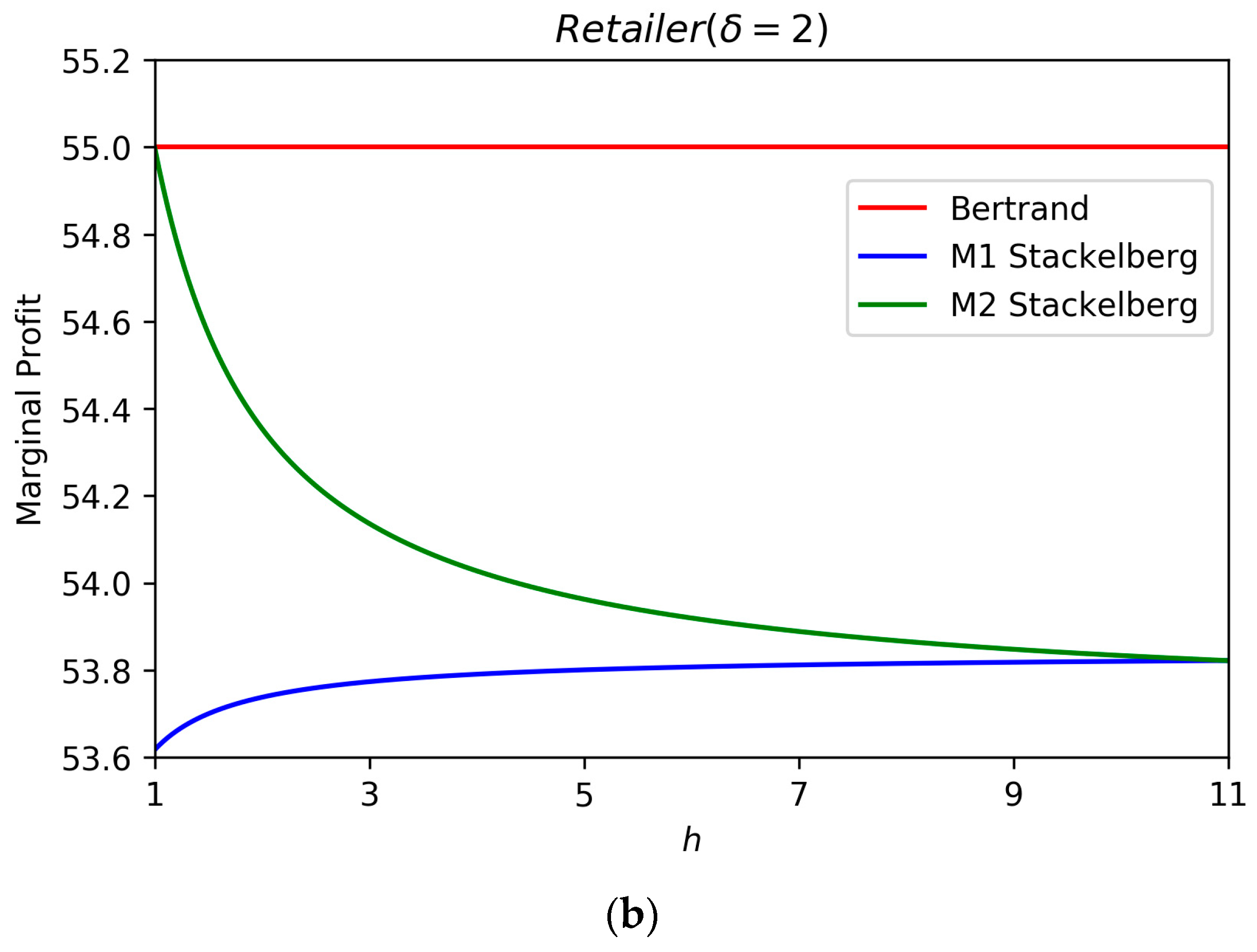
Figure 6 investigates the effect of
on players’ marginal profits under three sceneries. Different from
Figure 2a, manufacturer 1’s marginal profits are negative correlated with
, while manufacturer 2’s marginal profits are positive correlated with
. When the value of
is over than threshold (
,
and
), manufacturer 1’s marginal profits are lower than manufacturer 2’s (
,
and
). From
Figure 6b, the retailer’s total marginal profit is unrelated to parameter
in M1-M2 Bertrand model, is negative to
in M2-M1 Stackelberg model, but is positive to
in M1-M2 Stackelberg model. Furthermore, the retailer earns greatest in M1-M2 Bertrand model, second in M2-M1 Stackelberg and least in M1-M2 Stackelberg.
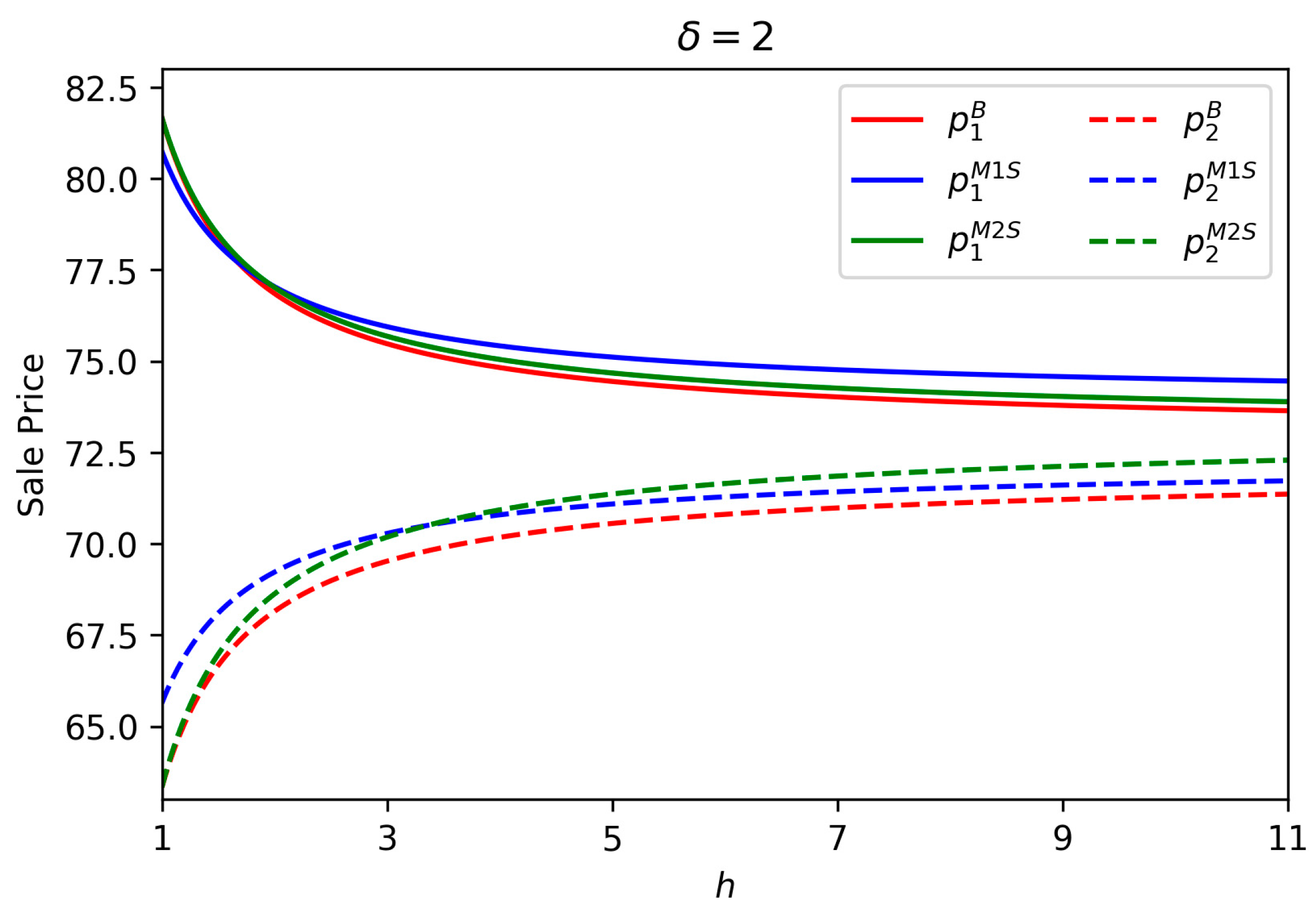
Figure 7 examines the effect of
on product sale prices under three sceneries.
Figure 7 probes the negative effects of
on sale price of product 1, and the positive effects on sale price of product 2. It is apparent that the sale prices of product 1 are always higher than product 2 in each sceneries and the gap narrows with the increase of
. This finding suggests that retailer should always set a higher price of green product than traditional product, however, the retailer should raise the sale price of traditional product but decrease the sale price of green product when greening cost effector rise.
Figure 8 scrutinizes the effect of
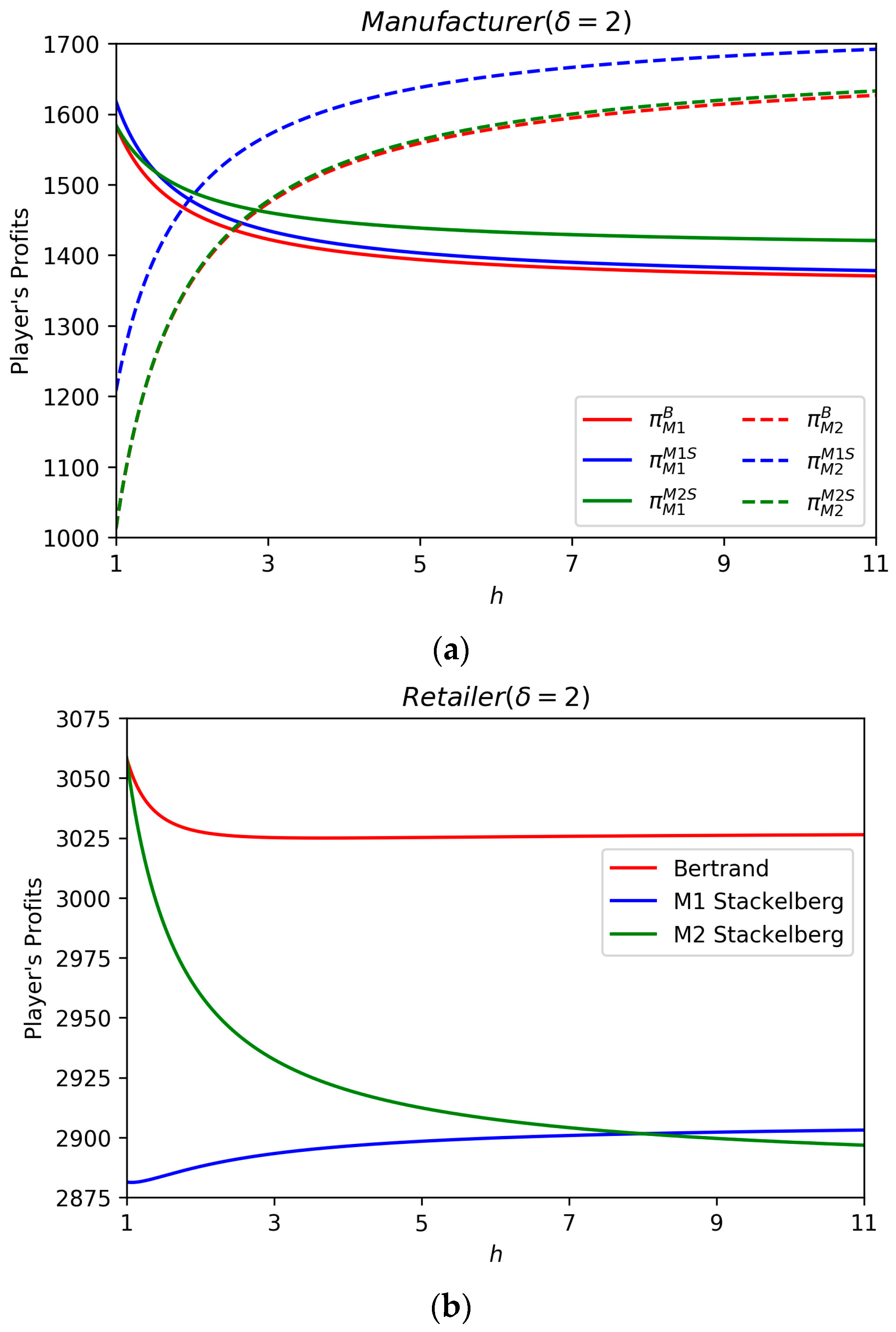
on players’ marginal profits under three sceneries.
Figure 8a explores the negative effects of
on manufacturer 1’s profit and the positive effects on manufacturer 2’s profit. Furthermore, manufacturer 2’s profit would surpass manufacturer 1’s profit with the increase of greening cost effector in each scenario. A great greening cost effector aggregates the burden of green producer and reduces its profit seriously, but encourages traditional manufacturer producing gray product. To motivate enterprises to be green participants, it is urgent to seek the financial supports from government and technical supports from third-party organizations. When the value of
exceeds the threshold, we find the formula
is tenable. This finding implicates that it is benefit for green manufacturer to be the leader of green market when green cost is at a low level, but to be the follower when greening cost is expensive. Further, it is easy to explore that the formula
is tenable. Similar to analyses in
Section 6.1, it is beneficial for traditional manufacturer to be follower in a green market. The correlations between the retailer’s total profit and
is complexed as demonstrated in
Figure 8b. In M1-M2 Bertrand game model, the retailer’s total profit decreases with the increase of
but it becomes steady when
outstrips a threshold. Furthermore, its total profit is positive to
in M2-oriented Stackelberg model, but negative in M1-oriented Stackelberg model. Further, the retailer earns the most in M1-M2 Bertrand game model, and whether the retailer prefers M1-oriented or M2-oriented Stackelberg game model depends on the value of
.
6. Conclusions and Future Research
6.1. Conclusions
The paper investigates the members’ optimal pricing policies and green strategies in the duopoly green supply chain. Three pricing game models are established through considering the manufacturers’ different market power, and the corresponding equilibrium solutions of these models are derived. Further, we conduct sensitive analysis of the main parameters and numerical example to compare the optimal pricing policies, greenness degree, the maximal profit margin and profits in three scenarios. The main findings are summarized as follows:
- (1)
With the level of the consumer’s environmental awareness increases, greenness degree of product will raise, the green manufacturer’s marginal profit and total profit will be enhanced, while traditional manufacturer’s marginal profit and total profit will be impaired in three sceneries. However, the retailer’s total profit will be increased in M1-M2 Bertrand game and M2-oriented Stackelberg game but be decreased in M1-oriented Stackelberg game.
- (2)
With the increment of greening cost effector, greenness degree of product decreases, the green manufacturer’s marginal profit and total profit will be impaired, while traditional manufacturer’s marginal profit and total profit will be enhanced in three sceneries. However, the retailer’s total profit will be decreased in M1-M2 Bertrand game and M2-oriented Stackelberg game but increased in M1-oriented Stackelberg game.
- (3)
The correlations of retailer’s total profit with respect to consumer’s environmental awareness and greening cost effector in the three scenarios is complexed. The retailer earns maximal total profit in M1-M2 Bertrand game, and the total profit increases with the increase of consumer’s environmental awareness but decreases with the increment of greening cost effector. When the consumer’s environmental awareness is over than a threshold, the retailer’s total profit in M2-oriented Stackelberg game is higher than total profit in M1-oriented Stackelberg game, and vice versa. When the greening cost effector exceeds the threshold, the retailer’s total profit M1 Stackelberg game is higher than in M2 Stackelberg game, and vice versa.
- (4)
The green competitive advantage is more effective than first-mover advantage while first-mover advantage does not be always effective in the green supply chain. Specially, traditional manufacturer always prefers to be the follower competing with the green manufacturer, which has no matter with the variety of consumer’s environmental awareness and greening cost effector, while green manufacturer would like to be the leader only when the consumer’s environmental awareness is relatively high or the greening cost coefficient is relatively low.
6.2. Future Directions
The paper only focuses on a two-stage green supply chain system with two manufacturers and one retailer. In fact, there are many other supply chain structures, e.g., dual channel supply chain and three-stage supply chain. Further, players’ risk attitudes are not taken into considered, which would affect manufacturers’ market strategies. Additionally, advertise strategy and sale effort should also be taken into consideration and their influences on members’ optimal decisions should be investigated either. Furthermore, the paper only considers the initial investment of green improvement, but ignores the overall greening costs especially in a long term, which might be an important decision variable of manufacturer’s green strategy. Besides, the integration of subjective consumer’s environmental awareness and overall greening cost is also worth to study.


