Retrieval of Sea Surface Temperature from MODIS Data in Coastal Waters


Abstract
1. Introduction
2. Materials
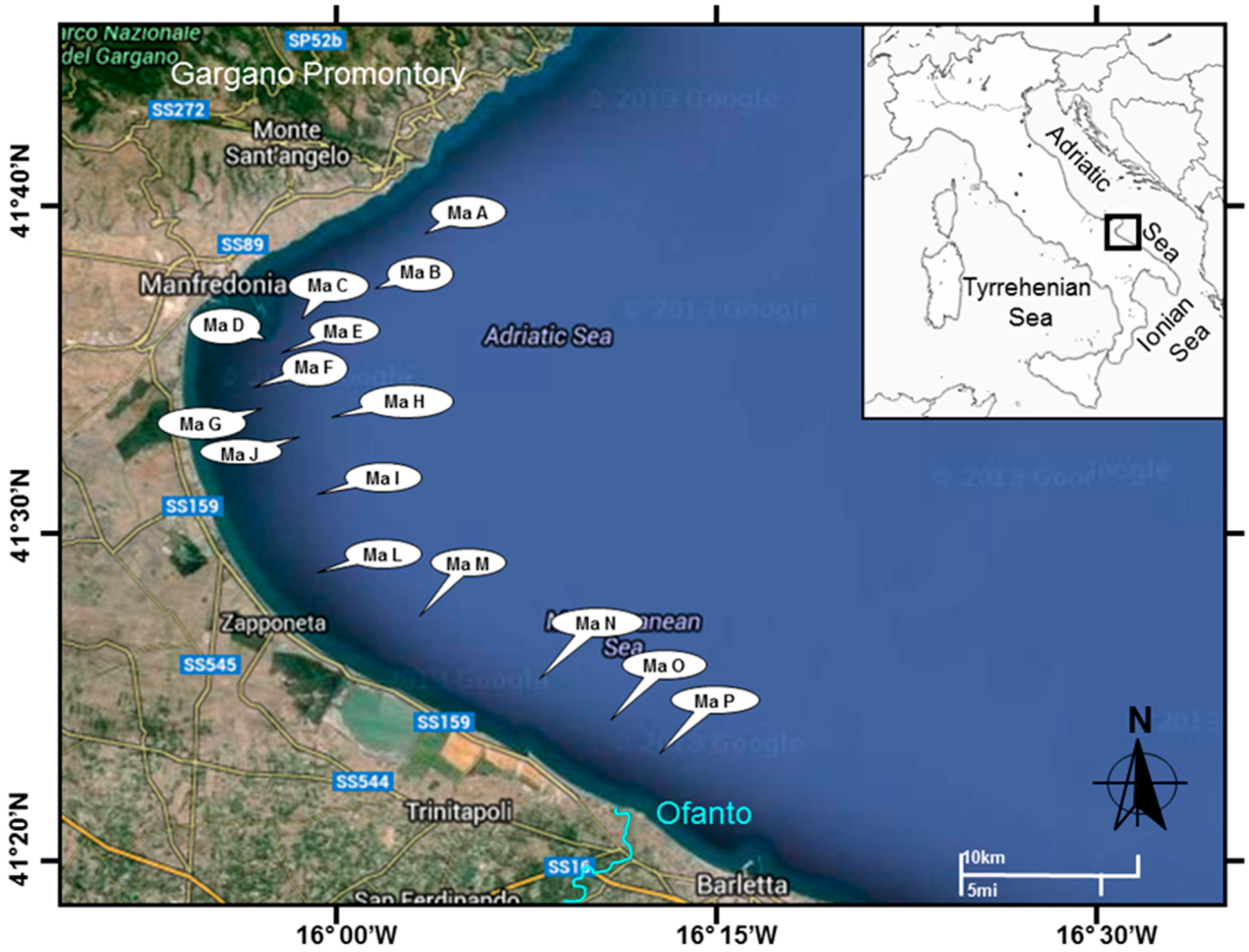
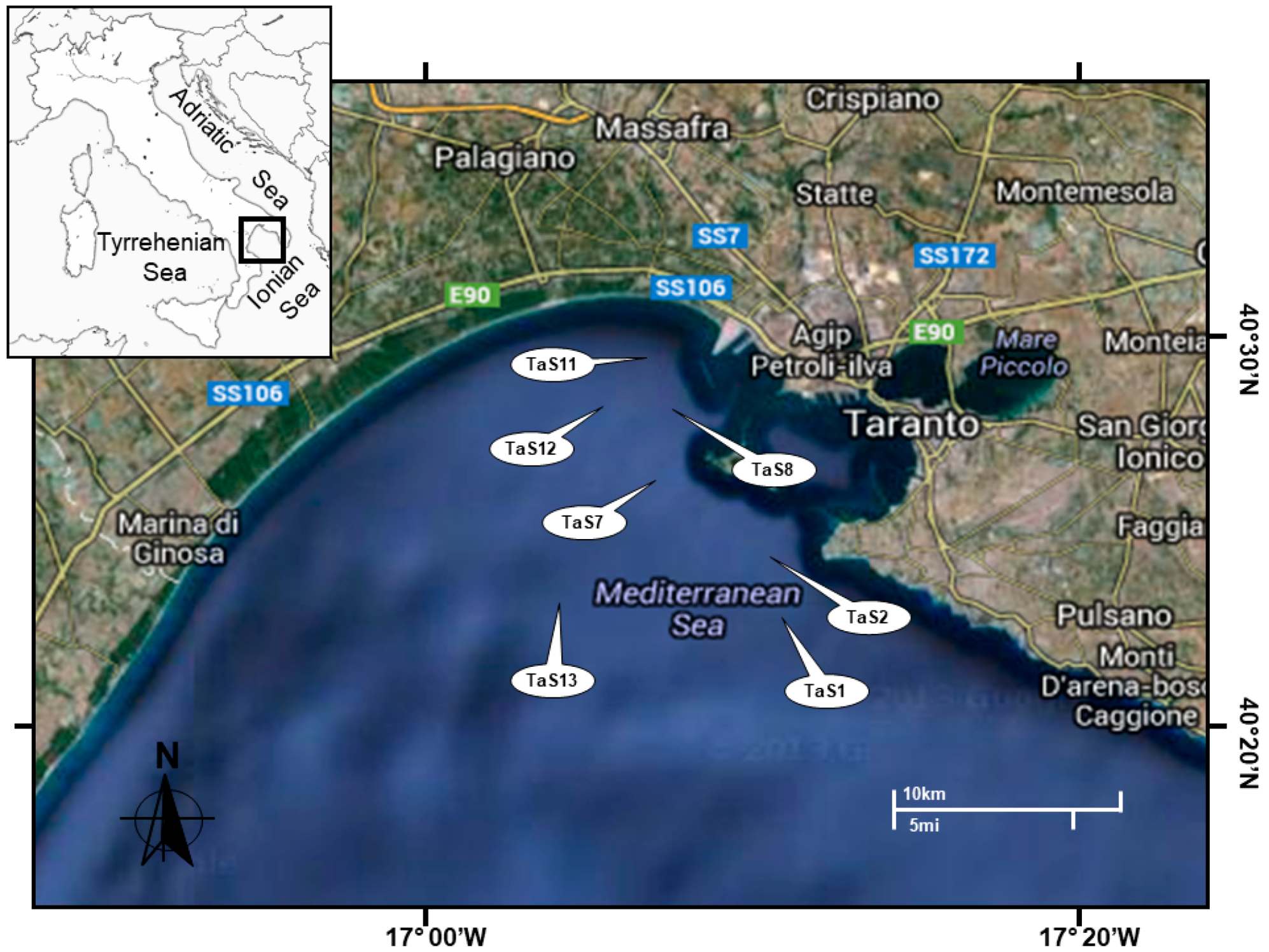
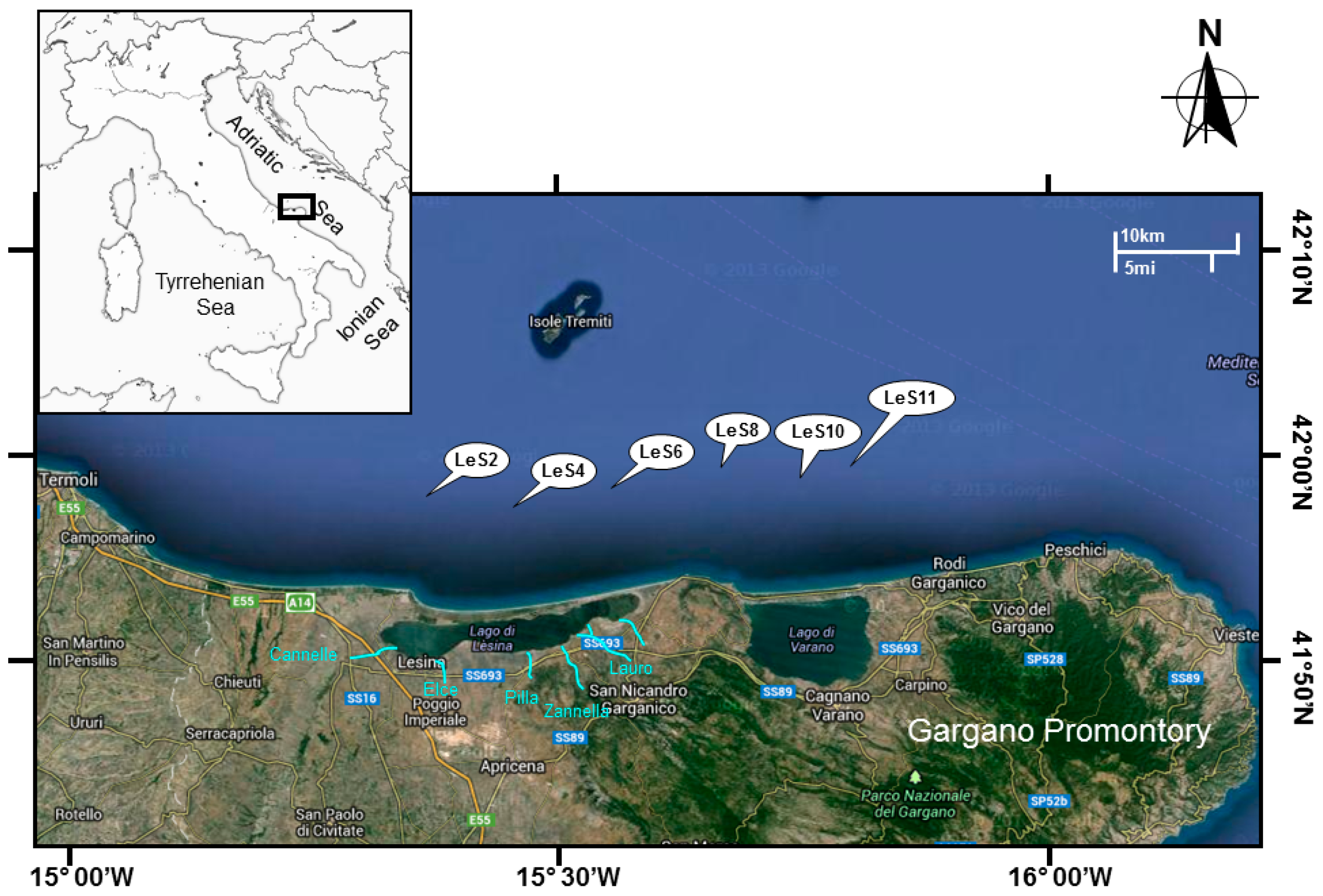
2.1. Study Area
2.2. In Situ and Satellite Data
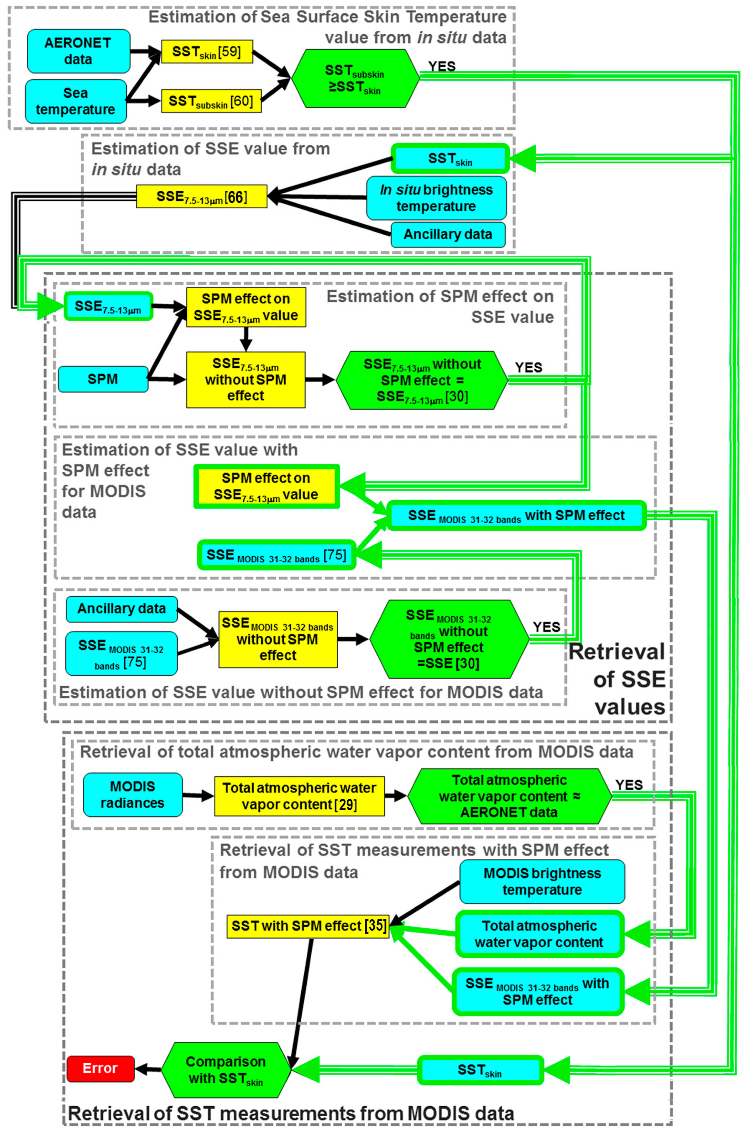
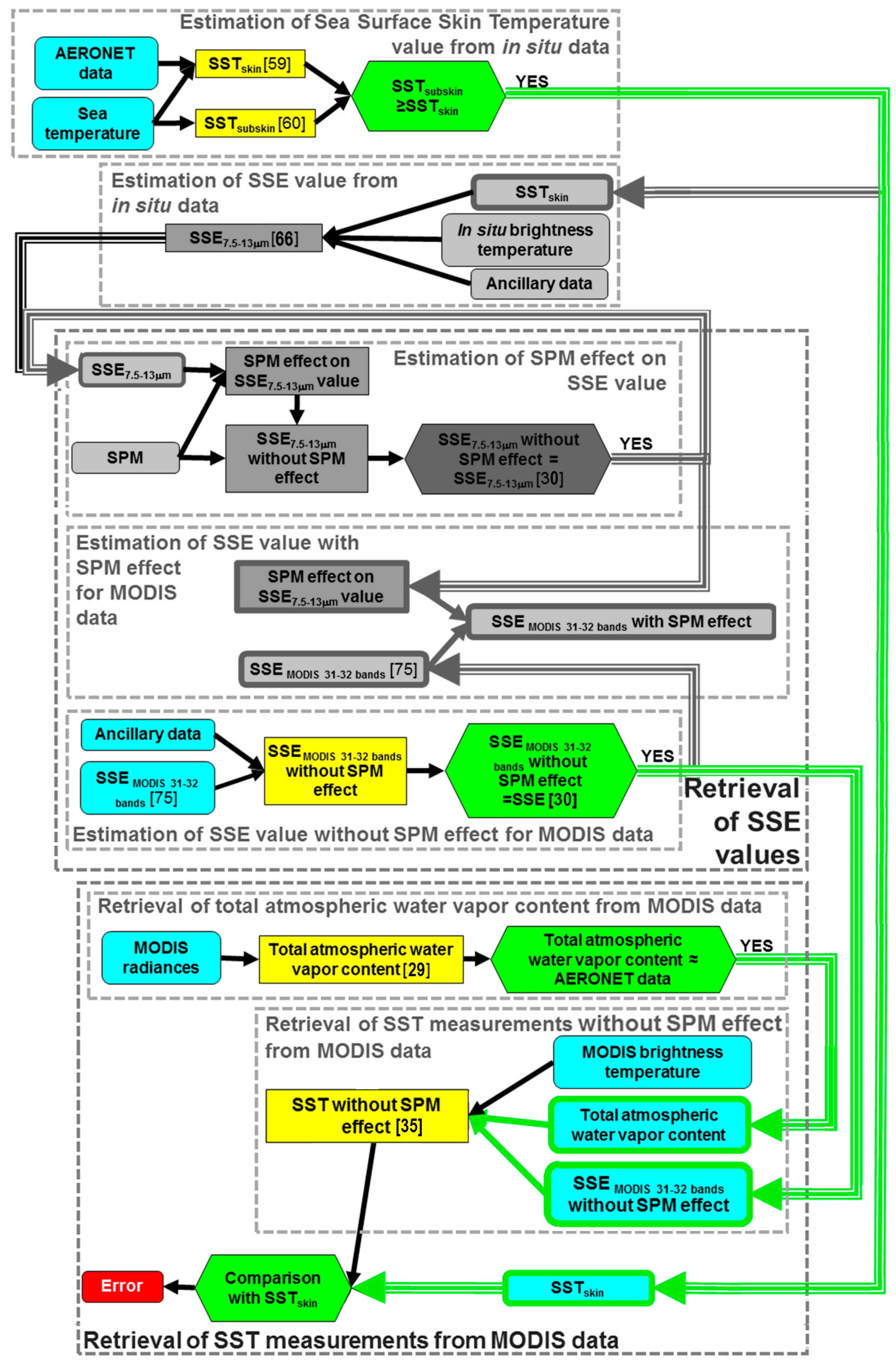
3. Estimation of Sea Surface Skin Temperature Value from in Situ Data
4. Estimation of SSE Value from in Situ Data
5. Retrieval of SSE Values
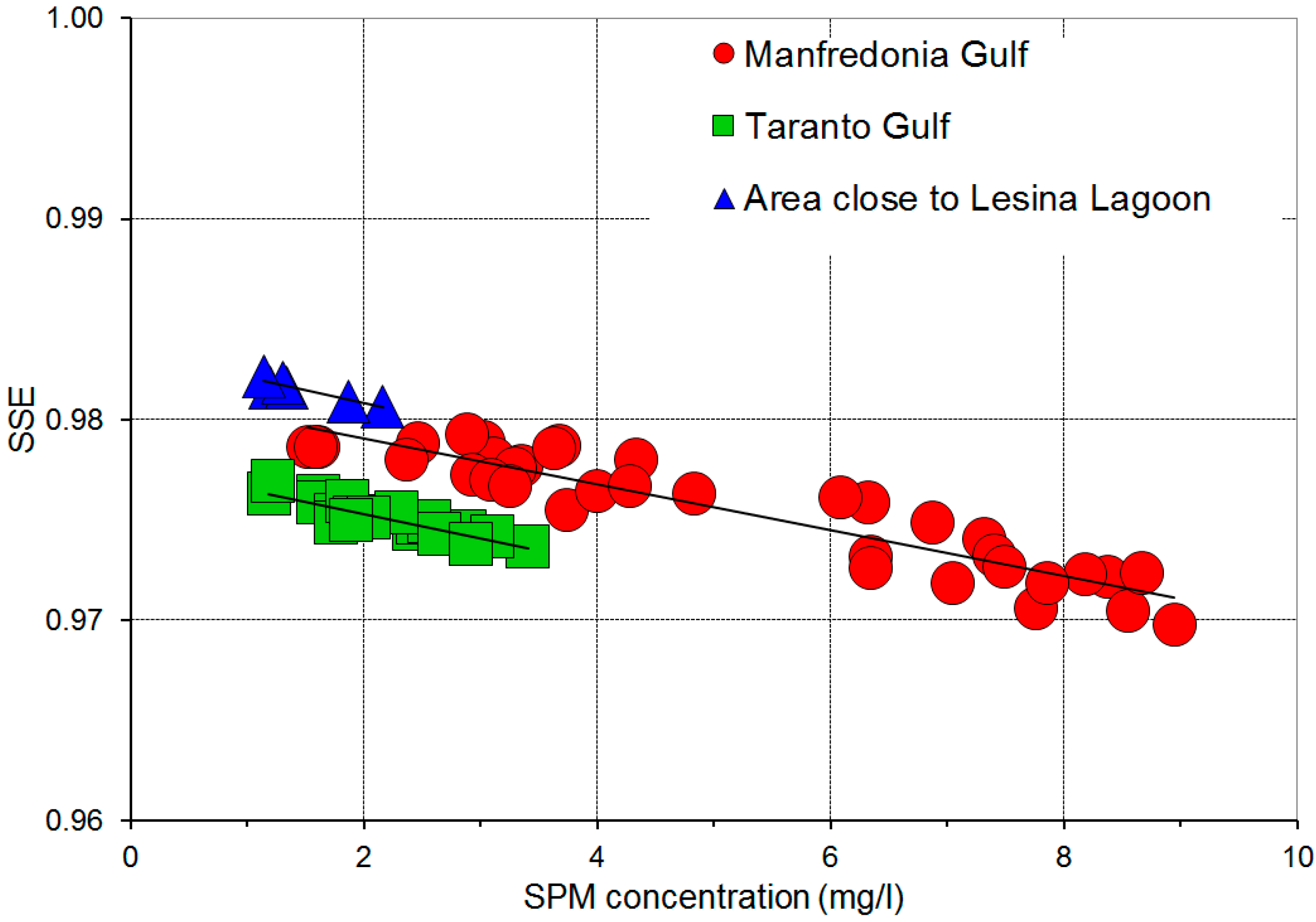
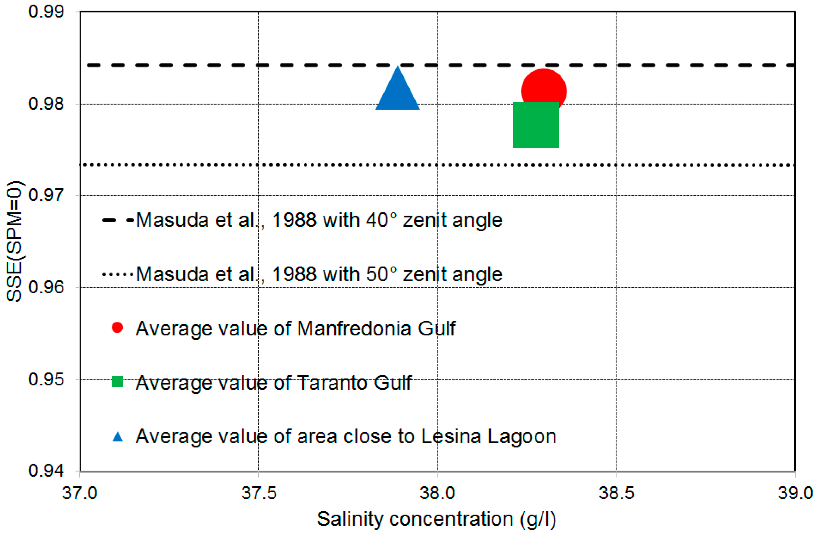
5.1. Estimation of SPM Effect on SSE Value
5.2. Estimation of SSE Value without SPM Effect for MODIS Data
6. Retrieval of SST Measurements from MODIS Data
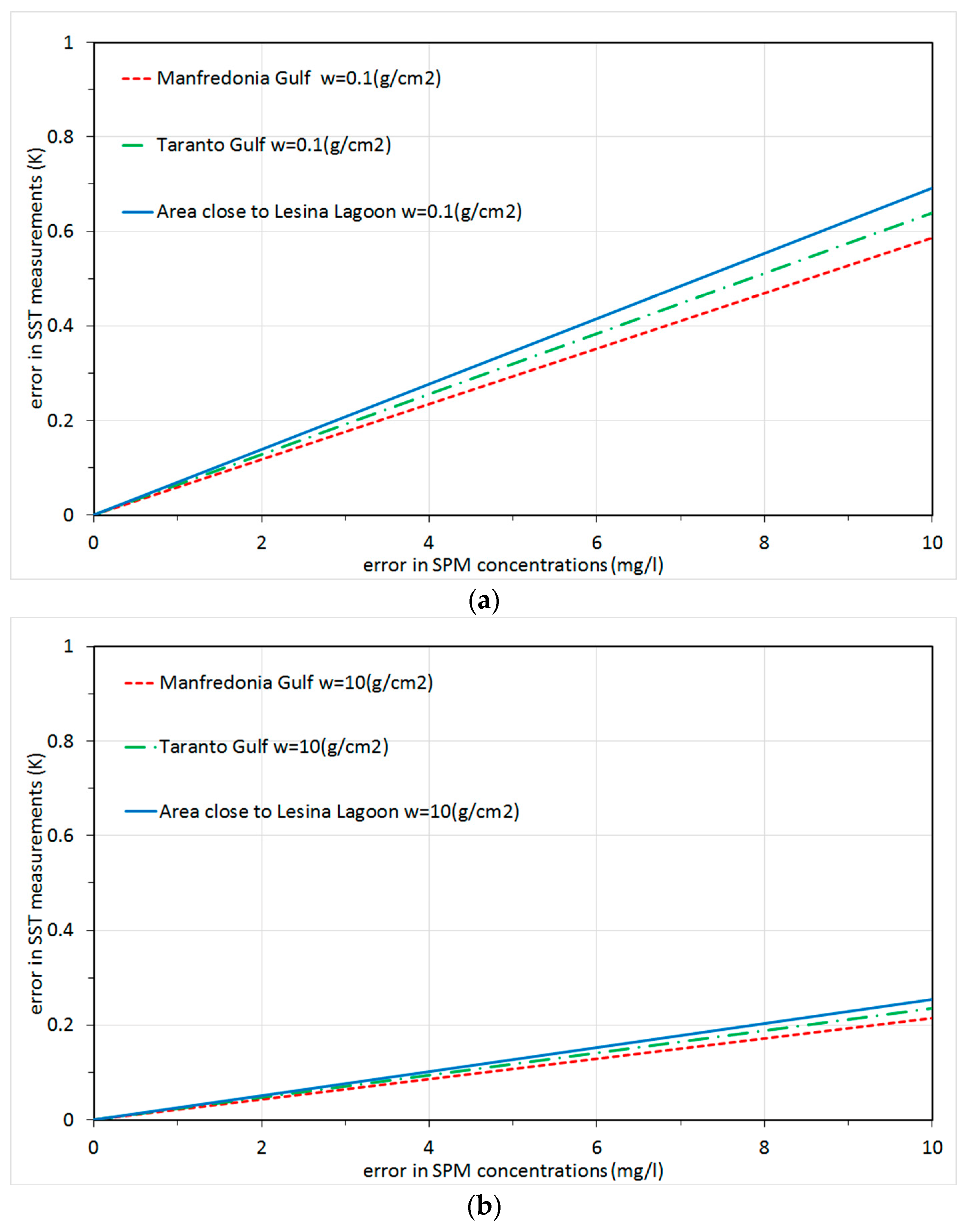
7. Sensitivity Analysis
8. Discussion and Conclusions
Acknowledgments
Conflicts of Interest
References
- Costanza, R.; de Groot, R.; Sutton, P.; van der Ploeg, S.; Anderson, S.J.; Kubiszewski, I.; Farber, S.; Turner, R.K. Changes in the global value of ecosystem services. Glob. Environ. Chang. 2014, 26, 152–158. [Google Scholar] [CrossRef]
- Crain, C.M.; Halpern, B.S.; Beck, M.W.; Kappel, C.V. Understanding and managing human threats to the coastal marine environment. Ann. N. Y. Acad. Sci. 2009, 1162, 39–62. [Google Scholar] [CrossRef] [PubMed]
- Ahuja, S. Monitoring Water Quality: Pollution Assessment, Analysis, and Remediation; Elsevier: Waltham, MA, USA, 2013; 379p. [Google Scholar]
- Sala, O.E.; Chapin, F.S.; Armesto, J.J.; Berlow, E.; Bloomfield, J.; Dirzo, R.; Leemans, R. Global biodiversity scenarios for the year 2100. Science 2000, 287, 1770–1774. [Google Scholar] [CrossRef]
- USCOP (US Commission on Ocean Policy). An Ocean Blueprint for the 21st Century: Final Report of the US Commission on Ocean Policy; US Commission on Ocean Policy: Washington, DC, USA, 2004. Available online: https://oceanconservancy.org/wp-content/uploads/2015/11/000_ocean_full_report-1.pdf (accessed on 31 July 2017).
- Blanchette, C.A.; Miner Melis, C.; Raimondi, P.T.; Lohse, D.; Heady, K.E.; Broitman, B.R. Biogeographical patterns of rocky intertidal communities along the Pacific coast of North America. J. Biogeogr. 2008, 35, 1593–1607. [Google Scholar] [CrossRef]
- Smale, D.A.; Wernberg, T. Satellite-derived SST data as a proxy for water temperature in nearshore benthic ecology. Mar. Ecol. Prog. Ser. 2009, 387, 27–37. [Google Scholar] [CrossRef]
- McCaul, M.; Barland, J.; Cleary, J.; Cahalane, C.; McCarthy, T.; Diamond, D. Combining Remote Temperature Sensing with in-Situ Sensing to Track Marine/Freshwater Mixing Dynamics. Sensors 2016, 16, 1402. [Google Scholar] [CrossRef] [PubMed]
- Thomas, A.; Byrne, D.; Weatherbee, R. Coastal sea surface temperature variability from Landsat infrared data. Remote Sens. Environ. 2002, 81, 262–272. [Google Scholar] [CrossRef]
- Fusilli, L.; Palombo, A.; Cavalli, R.M.; Pignatti, S. Airborne thermal data for detecting karst water resources in the Kotor Bay. In Proceedings of the 33rd International Symposium on Remote Sensing of Environment (ISRSE 2009), Stresa, Italy, 4–8 May 2009; pp. 356–359. [Google Scholar]
- De Boer, G.J.; Pietrzak, J.D.; Winterwerp, J.C. SST observations of upwelling induced by tidal straining in the Rhine ROFI. Cont. Shelf Res. 2009, 29, 263–277. [Google Scholar] [CrossRef]
- Ahn, Y.H.; Shanmugam, P.; Lee, J.H.; Kang, Y.Q. Application of satellite infrared data for mapping of thermal plume contamination in coastal ecosystem of Korea. Mar. Environ. Res. 2006, 61, 186–201. [Google Scholar] [CrossRef] [PubMed]
- Tang, D.; Kester, D.R.; Wang, Z.; Lian, J.; Kawamura, H. AVHRR satellite remote sensing and shipboard measurements of the thermal plume from the Daya Bay. nuclear power station. China. Remote Sen. Environ. 2003, 84, 506–515. [Google Scholar] [CrossRef]
- Xing, Q.; Chen, C.Q.; Shi, P. Method of integrating Landsat-5 and Landsat-7 data to retrieve sea surface temperature in coastal waters on the basis of local empirical algorithm. Ocean Sci. J. 2006, 41, 97–104. [Google Scholar] [CrossRef]
- Azzaro, F.; Cavalli, R.M.; Decembrini, F.; Pignatti, S.; Santella, C. Biochemical and dynamical characteristics of the Messina Straits water by means of hyperspectral data. In Proceedings of the Second International Asia-Pacific Symposium on Remote Sensing of the Atmosphere, Environment, and Space, Sendai, Japan, 23 January 2001; pp. 240–249. [Google Scholar] [CrossRef]
- Diofantos, G.H.; Marinos, G.H.; Kyriacos, T.; Agapiou, A. Integration of micro-sensor technology and remote sensing for monitoring coastal water quality in a municipal beach and other areas in Cyprus. In Proceedings of the SPIE Remote Sensing for Agriculture, Ecosystems, and Hydrology, Berlin, Germany, 18 September 2009. [Google Scholar]
- BIPM; IEC; IFCC; ILAC; ISO; IUPAC; IUPAP; OIML. Evaluation of Measurement Data—Guide to the Expression of Uncertainty in Measurement. International Organization for Standardization (ISO), 2008. Available online: http://www.bipm.org/en/publications/guides/gum.html (accessed on 31 July 2017).
- Smit, A.J.; Roberts, M.; Anderson, R.J.; Dufois, F.; Dudley, S.F.; Bornman, T.G.; Bolton, J.J. A Coastal Seawater Temperature Dataset for Biogeographical Studies: Large Biases between In Situ and Remotely-Sensed Data Sets around the Coast of South Africa. PLoS ONE 2013, 8, e81944. [Google Scholar] [CrossRef] [PubMed]
- Harries, J.E.; Llewellyn-Jones, D.T.; Minnett, P.J.; Saunders, R.W.; Zavody, A.M.; Wadhams, P.; Taylor, P.K.; Houghton, J.T. Observations of sea-surface temperature for climate research. Philos. Trans. R. Soc. Lond. A Math. Phys. Eng. Sci. 1983, 309, 381–395. [Google Scholar] [CrossRef]
- Esaias, W.E.; Abbott, M.R.; Barton, I.; Brown, O.B.; Campbell, J.W.; Carder, K.L.; Clark, D.K.; Evans, R.H.; Hoge, F.E.; Gordon, H.R.; et al. An overview of MODIS capabilities for ocean science observations. IEEE Trans. Geosci. Remote Sens. 1998, 36, 1250–1265. [Google Scholar] [CrossRef]
- Kilpatrick, K.A.; Podestá, G.; Walsh, S.; Williams, E.; Halliwell, V.; Szczodrak, M.; Brown, O.B.; Minnett, P.J.; Evans, R. A decade of sea surface temperature from MODIS. Remote Sens. Environ. 2015, 165, 27–41. [Google Scholar] [CrossRef]
- Liu, Y.; Minnett, P.J. Sampling errors in satellite-derived infrared sea-surface temperatures. Part I: Global and regional MODIS fields. Remote Sens. Environ. 2016, 177, 48–64. [Google Scholar] [CrossRef]
- Liu, Y.; Chin, T.M.; Minnett, P.J. Sampling errors in satellite-derived infrared sea-surface temperatures. Part II: Sensitivity and parameterization. Remote Sens. Environ. 2017, 198, 297–309. [Google Scholar] [CrossRef]
- Kilpatrick, K.A.; Podesta, G.P.; Evans, R. Overview of the NOAA/NASA advanced very high resolution radiometer Pathfinder algorithm for sea surface temperature and associated matchup database. J. Geophys. Res. Oceans 2001, 106, 9179–9197. [Google Scholar] [CrossRef]
- Brown, O.B.; Minnett, P.J.; Evans, R.; Kearns, E.; Kilpatrick, K.; Kumar, A.; Sikorski, R.; Závody, A. MODIS Infrared Sea Surface Temperature Algorithm Algorithm Theoretical Basis Document; Version 2.0; University of Miami: Coral Gables, FL, USA, 1999; 91p. [Google Scholar]
- Kennedy, J.J. A review of uncertainty in in situ measurements and data sets of sea surface temperature. Rev. Geophys. 2014, 52, 1–32. [Google Scholar] [CrossRef]
- Minnett, P.J.; Brown, O.B.; Evans, R.H.; Key, E.L.; Kearns, E.J.; Kilpatrick, K.; Kumar, A.; Maillet, K.A.; Szczodrak, G. Sea-surface temperature measurements from the Moderate-Resolution Imaging Spectroradiometer (MODIS) on Aqua and Terra. In Proceedings of the 2004 IEEE International Geoscience and Remote Sensing Symposium (IGARSS ’04), Anchorage, AK, USA, 20–24 September 2004; Volume 7, pp. 4576–4579. [Google Scholar] [CrossRef]
- Sobrino, J.A.; Li, Z.L.; Stoll, M.P. Impact of the atmospheric transmittance and total water vapor content in the algorithms for estimating satellite sea surface temperature. IEEE Trans. Geosci. Remote Sens. 1993, 31, 946–952. [Google Scholar] [CrossRef]
- Sobrino, J.A.; El Kharraz, J.; Li, Z.L. Surface temperature and water vapour retrieval from MODIS data. Int. J. Remote Sens. 2003, 24, 5161–5182. [Google Scholar] [CrossRef]
- Masuda, K.; Takashima, T.; Takayama, Y. Emissivity of pure and sea waters for the model sea surface in the infrared window regions. Remote Sens. Environ. 1988, 24, 313–329. [Google Scholar] [CrossRef]
- Konda, M.; Imasato, N.; Nishi, K.; Toda, T. Measurement of the sea surface emissivity. J. Oceanogr. 1994, 50, 17–30. [Google Scholar] [CrossRef]
- Kilpatrick, K.A. Climate Algorithm Theoretical Basis Document (C-ATBD): Pathfinder SST. CDRP-ATBD-0099 v2; 2013. Available online: http://www1.ncdc.noaa.gov/pub/data/sds/cdr/CDRs/Sea_Surface_Temperature_Pathfinder/AlgorithmDescription.pdf (accessed on 25 August 2017).
- Kilpatrick, K.; Podesta, G.; Walsh, S.; Evans, R.; Minnett, P. Implementation of Version 6 AQUA and TERRA SST Processing; White Paper; University of Miami: Coral Gables, FL, USA, 2014. [Google Scholar]
- McMillin, L.M. Estimation of sea surface temperatures from two infrared window measurements with different absorption. J. Geophys. Res. 1975, 80, 5113–5117. [Google Scholar] [CrossRef]
- Niclòs, R.; Caselles, V.; Coll, C.; Valor, E. Determination of sea surface temperature at large observation angles using an angular and emissivity-dependent split-window equation. Remote Sens. Environ. 2007, 111, 107–121. [Google Scholar] [CrossRef]
- Masuda, K. Influence of wind direction on the infrared sea surface emissivity model including multiple reflection effect. Meteorol. Geophys. 2012, 63, 1–13. [Google Scholar] [CrossRef]
- Niclòs, R.; Valor, E.; Caselles, V.; Coll, C.; Sánchez, J.M. In situ angular measurements of thermal infrared sea surface emissivity—Validation of models. Remote Sens. Environ. 2005, 94, 83–93. [Google Scholar] [CrossRef]
- Niclòs, R.; Caselles, V.; Valor, E.; Coll, C.; Sánchez, J.M. A simple equation for determing seasurface emissivity in the 3–15 µm region. Int. J. Remote Sens. 2009, 30. [Google Scholar] [CrossRef]
- Watts, P.D.; Allen, M.R.; Nightingale, T.J. Wind speed effects on sea surface emission and reflection for the along track scanning radiometer. J. Atmos. Ocean. Technol. 1996, 13, 126–141. [Google Scholar] [CrossRef]
- Wu, X.; Smith, W.L. Emissivity of rough sea surface for 8–13 µm: Modeling and verification. Appl. Opt. 1997, 36, 2609–2619. [Google Scholar] [CrossRef] [PubMed]
- Fiedler, L.; Bakan, S. Interferometric measurements of sea surface temperature and emissivity. Dtsch. Hydrogr. Z. 1997, 49, 357–365. [Google Scholar] [CrossRef]
- Newman, S.M.; Smith, J.A.; Glew, M.D.; Rogers, S.M.; Taylor, J.P. Temperature and salinity dependence of sea surface emissivity in the thermal infrared. Q. J. R. Meteorol. Soc. 2005, 131, 2539–2557. [Google Scholar] [CrossRef]
- Niclòs, R.; Caselles, V.; Coll, C.; Valor, E.; Rubto, E. Autonomous Measurements of Sea Surface Temperature Using In Situ Thermal Infrared Data. J. Atmos. Ocean. Technol. 2004, 21, 683–692. [Google Scholar] [CrossRef]
- Smith, W.L.; Knuteson, R.O.; Revercomb, H.E.; Feltz, W.; Howell, H.B.; Menzel, W.P.; Nalli, N.R.; Brown, O.; Brown, J.; Minnett, P.; et al. Observations of the infrared radiative properties of the ocean-implications for the measurement of sea surface temperature via satellite remote sensing. Bull. Am. Meteorol. Soc. 1996, 77, 41–51. [Google Scholar] [CrossRef]
- Cox, C.; Munk, W. Measurement of the roughness of the sea surface from photographs of the sun’s glitter. JOSA 1954, 44, 838–850. [Google Scholar] [CrossRef]
- Wen-Yao, L.; Field, R.T.; Gantt, R.G.; Klemas, V. Measurement of the surface emissivity of turbid waters. Remote Sens. Environ. 1987, 21, 97–109. [Google Scholar] [CrossRef]
- Salisbury, J.W. Emissivity of terrestrial materials in the 8–14 μm atmospheric window. Remote Sens. Environ. 1992, 42, 83–106. [Google Scholar] [CrossRef]
- Park, J.H.; Na, S.I. SST and SS changes during Saemangeum seawall construction using Landsat TM and ETM imagery. Proc. SPIE 2010, 7831. [Google Scholar] [CrossRef]
- Wei, J.A.; Wang, D.; Gong, F.; He, X.; Bai, Y. The Influence of Increasing Water Turbidity on Sea Surface Emissivity. IEEE Trans. Geosci. Remote Sens. 2017, 55, 3501–3515. [Google Scholar] [CrossRef]
- Zhao, Y.S. Principles and Methods of Remote Sensing Application; Science Press: Beijing, China, 2003. [Google Scholar]
- Morel, A. Optical modelling of the upper ocean in relation to its biogenous matter content (case 1 waters). J. Geophys. Res. 1988, 93, 10749–10768. [Google Scholar] [CrossRef]
- Mueller, J.L.; Austin, R.W.; Morel, A.; Fargion, G.S.; McClain, C.R. Ocean Optics Protocols for Satellite Ocean Color Sensor Validation. Volume I: Introduction. Background and Conventions; Revision 4, NASA Tech. Memo. 2003-21621; NASA Goddard Space Flight Center: Greenbelt, MD, USA, 2003; pp. 1–56.
- Cavalli, R.M.; Betti, M.; Campanelli, A.; Di Cicco, A.; Guglietta, D.; Penna, P.; Piermattei, V. A methodology to assess the accuracy with which remote data characterize a specific surface, as a Function of Full Width at Half Maximum (FWHM): Application to three Italian coastal waters. Sensors 2014, 14, 1155–1183. [Google Scholar] [CrossRef] [PubMed]
- Fiesoletti, F.; Specchiulli, A.; Spagnoli, F.; Zappalà, G. A new near time monitoring network in the Gulf of Manfredonia-Southern Adriatic Sea. In European Operational Oceanography: Present and Future, Proceedings of the 4th International Conference on EuroGOOS, Brest, France, 6–9 June 2005; European Commission Research Directorate-General: Brussels, Belgium, 2005; pp. 782–792. [Google Scholar]
- Meftah, M.B.; De Serio, F.; Mossa, M.; Petrillo, A.F.; Pollio, A. Numerical results of the pollutant spreading offshore Taranto (Italy). In Proceedings of the 33rd IAHR Congress: Water Engineering for a Sustainable Environment, Vancouver, BC, Canada, 9–14 August 2009. [Google Scholar]
- Law n. 349 (1986). Istituzione del Ministero Dell’ambiente e Norme in Materia di Danno Ambientale. Gazzetta Ufficiale della Repubblica Italiana del 15 luglio 1986, n. 162, Supplemento Ordinario n. 59. Available online: http://www.minambiente.it/sites/default/files/legge_08_07_1986_349.pdf (accessed on 6 November 2017).
- Law n. 426 (1998). Nuovi interventi in campo ambientale. Gazzetta Ufficiale della Repubblica Italiana del 14 Dicembre 1998, n. 291, Serie Generale. Available online: http://www.agentifisici.isprambiente.it/ (accessed on 6 November 2017).
- Roselli, L.; Fabbrocini, A.; Manzo, C.; D’Adamo, R. Hydrological heterogeneity. nutrient dynamics and water quality of a non-tidal lentic eco system (Lesina Lagoon. Italy). Estuar. Coast. Shelf Sci. 2009, 84, 539–552. [Google Scholar] [CrossRef]
- Webster, P.J.; Clayson, C.A.; Curry, J.A. Clouds, radiation, and the diurnal cycle of sea surface temperature in the tropical western Pacific. J. Clim. 1996, 9, 1712–1730. [Google Scholar] [CrossRef]
- Fairall, C.W.; Bradley, E.F.; Hare, J.E.; Grachev, A.A.; Edson, J.B. Bulk parameterization of air–sea fluxes: Updates and verification for the COARE algorithm. J. Clim. 2003, 16, 571–591. [Google Scholar] [CrossRef]
- Mueller, J.L.; McClain, G.; Bidigare, R.; Trees, C.; Balch, W.; Dore, J.; Drapeau, D.; Karl, D.; Van, L. Ocean Optics Protocols for Satellite Ocean Color Sensor Validation. Revision 5. Volume V: Biogeochemical and Bio-Optical Measurements and Data Analysis Protocols; NASA Tech. Memo. 2003-21621; NASA Goddard Space Flight Center: Greenbelt, MD, USA, 2003; pp. 1–36.
- Pegau, S.; Zaneveld, J.R.V.; Mitchell, B.G.; Mueller, J.L.; Kahru, M.; Wieland, J.; Stramska, M. Ocean Optics Protocols For Satellite Ocean Color Sensor Validation. Revision 4. Volume IV: Inherent Optical Properties: Instruments. Characterizations. Field Measurements and Data Analysis Protocols; NASA Tech. Memo. 2003-211621; NASA Goddard Space Flight Center: Greenbelt, MD, USA, 2003; pp. 1–76.
- Bonamano, S.; Piermattei, V.; Marcelli, M.; Peviani, M. Comparison Between Physical Variables Acquired by a New Multiparametric Platform, ELFO, and Data Calculated by a Three-Dimensional Hydrodynamic Model in Different Weather Conditions at Tiber River mouth (Latium coast, Italy). EGU General Assembly Conference Abstracts, May 2010; Volume 12, p. 5226. Available online: http://meetingorganizer.copernicus.org/EGU2010/EGU2010-5226.pdf (accessed on 31 July 2017).
- Marcelli, M.; Piermattei, V.; Madonia, A.; Lacava, T.; Mainardi, U. T-FLaP advances: Instrumental and operative implementation. J. Oper. Oceanogr. 2016, 9, s185–s192. [Google Scholar] [CrossRef]
- Crease, J.; Dauphinee, T.; Grose, P.L.; Lewis, E.L.; Fofonoff, N.P.; Plakhin, E.A.; Striggow, K.; Zenk, W. The Acquisition. Calibration and Analysis of CTD Data; UNESCO Technical Papers in Marine Sciences, 54; UNESCO: Paris, France, 1988; pp. 1–105. [Google Scholar]
- User’s Manual Thermal CAM Reseacher Professional—Professional Edition; Version 2.9; FLIR Systems: Limbiate (MI), Italy, 2009.
- Mueller, J.L.; Morel, A.; Frouin, R.; Davis, C.; Arnone, R.; Carder, K.; Lee, Z.P.; Steward, R.G.; Hooker, S.; Holben, B.; et al. Ocean Optics Protocols For Satellite Ocean Color Sensor Validation. Revision 4. Volume III: Radiometric Measurements and Data Analysis Protocols; NASA Tech. Memo. 2003-21621; NASA Goddard Space Flight Center: Greenbelt, MD, USA, 2003; pp. 1–84.
- Donlon, C.; Rayner, N.; Robinson, I.; Poulter, D.J.S.; Casey, K.S.; Vazquez-Cuervo, J.; May, D. The global ocean data assimilation experiment high-resolution sea surface temperature pilot project. Bull. Am. Meteorol. Soc. 2007, 88, 1197–1213. [Google Scholar] [CrossRef]
- Donlon, C.J.; Minnett, P.J.; Gentemann, C.; Nightingale, T.J.; Barton, I.J.; Ward, B.; Murray, M.J. Toward improved validation of satellite sea surface skin temperature measurements for climate research. J. Clim. 2002, 15, 353–369. [Google Scholar] [CrossRef]
- Donlon, C.J.; Keogh, S.J.; Baldwin, D.J.; Robinson, I.S.; Ridley, I.; Sheasby, T.; Barton, I.J.; Bradley, E.F.; Nightingale, T.J.; Emery, W. Solid-State Radiometer Measurements of Sea Surface Skin Temperature. J. Atmos. Ocean. Technol. 1998, 15, 775–787. [Google Scholar] [CrossRef]
- Kawai, Y.; Wada, A. Diurnal sea surface temperature variation and its impact on the atmosphere and ocean: A review. J. Oceanogr. 2007, 63, 721–744. [Google Scholar] [CrossRef]
- Fairall, C.W.; Bradley, E.F.; Godfrey, J.S.; Wick, G.A.; Edson, J.B.; Young, G.S. Cool-skin and warm-layer effects on sea surface temperature. J. Geophys. Res. Oceans 1996, 101, 1295–1308. [Google Scholar] [CrossRef]
- Gentemann, C.L.; Minnett, P.J.; Ward, B. Profiles of ocean surface heating (POSH): A new model of upper ocean diurnal warming. J. Geophys. Res. Oceans 2009, 114, C07017. [Google Scholar] [CrossRef]
- Zeng, X.; Beljaars, A. A prognostic scheme of sea surface skin temperature for modeling and data assimilation. Geophys. Res. Lett. 2005, 32, L14605. [Google Scholar] [CrossRef]
- Niclòs, R.; Caselles, V. Angular variation of the sea surface emissivity. In Recent Research Development in Thermal Remote Sensing; Research Signpost: Kerela, Indian, 2005; pp. 37–65. [Google Scholar]
- Friedman, D. Infrared characteristics of ocean water (1.5–15 μ). Appl. Opt. 1969, 8, 2073–2078. [Google Scholar] [CrossRef] [PubMed]
- PO.DAAC MODIS Level 3 Data User Guide, MODIS Dataset, Version 2014.0. Available online: ftp://podaac-ftp.jpl.nasa.gov/allData/modis/L3/docs/UserGuide_MODIS_L3_v2014.0.pdf (accessed on 1 February 2017).
- Mavromatakis, F.; Gueymard, C.A.; Franghiadakis, Y. Improved total atmospheric water vapour amount determination from near-infrared filter measurements with sun photometers. Atmos. Chem. Phys. 2007, 7, 4613–4623. [Google Scholar] [CrossRef]
- Polemio, M.; Dragone, V.; Limoni, P.P. Monitoring and methods to analyse the groundwater quality degradation risk in coastal karstic aquifers (Apulia, Southern Italy). Environ. Geol. 2009, 58, 299–312. [Google Scholar] [CrossRef]
- Simeoni, U. I litorali tra Manfredonia e Barletta (Basso Adriatico): Dissesti, sedimenti, problematiche ambientali. Boll. Soc. Geol. Ital. 1992, 111, 367–398. [Google Scholar]
- Korzybski, A. Science and Sanity; Science Press Printing: Lancaster, PA, USA, 1958. [Google Scholar]
- Milella, M. Esplorare le Frontiere verso una Interculturalitá Formativa; Edizione Ateneo: Perugia, Italy, 2007. [Google Scholar]


| Coastal Waters of the Area Close to Lesina Lagoon | |||||
| Date | Start time (UTC) | End time (UTC) | Number of locations | Mean of SSTSkin by [59] (K) | Mean of SSTsubskin by [60] (K) |
| 07 August 2011 | 7:30 | 16:00 | 6 | 300.12 | 300.14 |
| Coastal Waters of the Manfredonia Gulf | |||||
| Date | Start time (UTC) | End time (UTC) | Number of Locations | Mean of SSTSkin by [59] (K) | Mean of SSTsubskin by [60] (K) |
| 08 August 2011 | 7:01 | 15:20 | 6 | 301.25 | 301.27 |
| 09 August 2011 | 6:30 | 15:00 | 9 | 301.15 | 301.26 |
| 12 August 2011 | 7:50 | 16:10 | 10 | 299.79 | 299.99 |
| 24 August 2011 | 5:40 | 17:30 | 14 | 301.86 | 302.05 |
| Coastal Waters of the Taranto Gulf | |||||
| Date | Start time (UTC) | End time (UTC) | Number of Locations | Mean of SSTSkin by [59] (K) | Mean of SSTsubskin by [60] (K) |
| 13 August 2011 | 11:00 | 15:10 | 5 | 299.46 | 299.59 |
| 14 August 2011 | 7:05 | 14:30 | 7 | 300.25 | 300.34 |
| 15 August 2011 | 7:00 | 14:00 | 7 | 299.81 | 299.99 |
| 16 August 2011 | 10:00 | 14:00 | 2 | 299.95 | 300.02 |
| Coastal Waters of | SPM (mg/L) | Salinity (g/L) | SSE (SPM ≠ 0) | SSE (SPM = 0) | ||||
|---|---|---|---|---|---|---|---|---|
| Mean | σ | Mean | σ | Mean | σ | Mean | σ | |
| the Manfredonia Gulf | 5.07 | 2.36 | 38.30 | 0.11 | 0.975 | 0.003 | 0.981 | 0.003 |
| the Taranto Gulf | 2.15 | 0.60 | 38.30 | 0.04 | 0.975 | 0.001 | 0.978 | 0.001 |
| area close to Lesina Lagoon | 1.50 | 0.41 | 37.86 | 0.08 | 0.981 | 0.001 | 0.984 | 0.001 |
| Coastal Waters of the Area Close to Lesina Lagoon | |||||
| Date Start Time | W (g/cm2) | Number of Locations | Number of Locations Obtained from MODIS Level 3 | SST (K) | |
| MODIS Level 3 | |||||
| 07 August 2011 12:40 UTC | 1.563 | 6 | 6 | Bias | 1.43 |
| σ | 0.44 | ||||
| RMSD | 1.49 | ||||
| Coastal Waters of the Manfredonia Gulf | |||||
| Date Start Time | W (g/cm2) | Number of locations | Number of Locations Obtained from MODIS Level 3 | SST (K) | |
| MODIS Level 3 | |||||
| 08 August 2011 11:45 UTC | 5.246 | 5 | 2 | Bias | 1.12 |
| σ | 0.64 | ||||
| RMSD | 1.21 | ||||
| 09 August 2011 12:25 UTC | 10.655 | 7 | 1 | Bias | 1.36 |
| σ | - | ||||
| RMSD | - | ||||
| 12 August 2011 11:20 UTC | 0.743 | 8 | 8 | Bias | 1.11 |
| σ | 0.39 | ||||
| RMSD | 1.17 | ||||
| 24 August 2011 11:40 UTC | 2.103 | 11 | 7 | Bias | 0.20 |
| σ | 0.11 | ||||
| RMSD | 1.26 | ||||
| Coastal Waters of Taranto Gulf | |||||
| Date Start Time | W (g/cm2) | Number of Locations | Number of Locations Obtained from MODIS Level 3 | SST (K) | |
| MODIS Level 3 | |||||
| 13 August 2011 12:00 UTC | 1.370 | 5 | 5 | Bias | 1.41 |
| σ | 0.31 | ||||
| RMSD | 1.31 | ||||
| 14 August 2011 12:45 UTC | 1.517 | 6 | 1 | Bias | 1.33 |
| σ | - | ||||
| RMSD | - | ||||
| 15 August 2011 11:50 UTC | 0.743 | 6 | 7 | Bias | 0.98 |
| σ | 0.43 | ||||
| RMSD | 1.06 | ||||
| 16 August 2011 12:30 UTC | 1.197 | 2 | 1 | Bias | 0.44 |
| σ | - | ||||
| RMSD | - | ||||
| Coastal Waters of the Area Close to Lesina Lagoon | ||||||
| Date Start Time | W (g/cm2) | Number of Locations | SST (K) Retrieved by [35] | |||
| with SSE (SPM = 0) | with SSE (SPM ≠ 0) Using Equations (7)–(9) | with SSE (SPM ≠ 0) Using Wen-Yao et al. [46] | ||||
| 07 August 2011 12:40 UTC | 1.563 | 6 | Bias | −0.49 | −0.40 | −0.49 |
| σ | 0.48 | 0.50 | 0.48 | |||
| RMSD | 0.66 | 0.60 | 0.66 | |||
| Coastal Waters of the Manfredonia Gulf | ||||||
| Date Start Time | W (g/cm2) | Number of Locations | SST (K) Retrieved by [35] | |||
| with SSE (SPM = 0) | with SSE (SPM ≠ 0) Using Equations (7)–(9) | with SSE (SPM ≠ 0) Using Wen-Yao et al. [46] | ||||
| 08 August 2011 11:45 UTC | 5.246 | 5 | Bias | −0.80 | −0.65 | −0.72 |
| σ | 0.48 | 0.43 | 0.43 | |||
| RMSD | 0.91 | 0.76 | 0.82 | |||
| 09 August 2011 12:25 UTC | 10.655 | 7 | Bias | −0.73 | −0.67 | −0.72 |
| σ | 1.09 | 1.09 | 1.09 | |||
| RMSD | 1.26 | 1.23 | 1.26 | |||
| 12 August 2011 11:20 UTC | 0.743 | 8 | Bias | −0.81 | −0.50 | −0.79 |
| σ | 0.52 | 0.46 | 0.52 | |||
| RMSD | 0.95 | 0.66 | 0.93 | |||
| 24 August 2011 11:40 UTC | 2.103 | 11 | Bias | −0.71 | −0.29 | −0.69 |
| σ | 0.31 | 0.31 | 0.31 | |||
| RMSD | 0.77 | 0.42 | 0.75 | |||
| Coastal Waters of Taranto Gulf | ||||||
| Date Start Time | W (g/cm2) | Number of Locations | SST (K) Retrieved by [35] | |||
| with SSE (SPM = 0) | with SSE (SPM ≠ 0) Using Equations (7)–(9) | with SSE (SPM ≠ 0) Using Wen-Yao et al. [46] | ||||
| 13 August 2011 12:00 UTC | 1.370 | 5 | Bias | −1.03 | −0.89 | −1.03 |
| σ | 0.12 | 0.15 | 0.12 | |||
| RMSD | 1.04 | 0.89 | 1.03 | |||
| 14 August 2011 12:45 UTC | 1.517 | 6 | Bias | −0.54 | −0.42 | −0.54 |
| σ | 0.25 | 0.24 | 0.25 | |||
| RMSD | 0.59 | 0.48 | 0.59 | |||
| 15 August 2011 11:50 UTC | 0.743 | 6 | Bias | −0.73 | −0.59 | −0.72 |
| σ | 0.31 | 0.31 | 0.32 | |||
| RMSD | 0.78 | 0.65 | 0.78 | |||
| 16 August 2011 12:30 UTC | 1.197 | 2 | Bias | −0.52 | −0.41 | −0.51 |
| σ | 0.07 | 0.08 | 0.07 | |||
| RMSD | 0.52 | 0.42 | 0.52 | |||
© 2017 by the author. Licensee MDPI, Basel, Switzerland. This article is an open access article distributed under the terms and conditions of the Creative Commons Attribution (CC BY) license (http://creativecommons.org/licenses/by/4.0/).
Share and Cite
Cavalli, R.M. Retrieval of Sea Surface Temperature from MODIS Data in Coastal Waters. Sustainability 2017, 9, 2032. https://doi.org/10.3390/su9112032
Cavalli RM. Retrieval of Sea Surface Temperature from MODIS Data in Coastal Waters. Sustainability. 2017; 9(11):2032. https://doi.org/10.3390/su9112032
Chicago/Turabian StyleCavalli, Rosa Maria. 2017. "Retrieval of Sea Surface Temperature from MODIS Data in Coastal Waters" Sustainability 9, no. 11: 2032. https://doi.org/10.3390/su9112032
APA StyleCavalli, R. M. (2017). Retrieval of Sea Surface Temperature from MODIS Data in Coastal Waters. Sustainability, 9(11), 2032. https://doi.org/10.3390/su9112032