An Assessment of Productivity Patterns of Grass-Dominated Rangelands in the Hindu Kush Karakoram Region, Pakistan

Abstract

Rangelands in the Hindu Kush Karakoram region provide a resource base for nomadic livestock grazing, which is one of the major traditional livelihood practices in the area. The present study assessed the spatiotemporal patterns and trends of rangelands using satellite remote-sensing time-series data. Moderate resolution imaging spectroradiometer (MODIS)-based normalized difference vegetation index (NDVI) data, collected at fortnightly intervals over 12 years (2001–2012), were used as a proxy for the vegetation conditions of the grasslands. The analysis revealed that rangeland productivity increased with increasing elevation up to the sub-alpine zone, which had a higher productivity than the moist temperate zone and humid sub-tropical zone. The high sub-alpine productivity was attributed to seasonal amplitude and the extended length of the growing season in the phenological cycle. In the temporal analysis of productivity, the majority of the area exhibited improvements in vegetation conditions, which were strongest in the humid sub-tropical zones and weakest in the alpine zones. The sub-alpine grasslands were found to be the most productive and heterogeneous habitat; however, the relatively strong negative temporal trend in productivity in this zone indicates ongoing degradation in these rangelands. Thus, special attention is needed for the sustainable management of rangelands in the sub-alpine zones of the Hindu Kush Karakoram region.

1. Introduction

The sustainability of rangelands is one of the central issues in context of contemporary environmental changes. However, understanding rangeland dynamics is a contentious issue, and there is some debate as to whether the dynamics of arid, semi-arid and sub-humid rangelands are driven by anthropogenic factors (mainly grazing pressure), as suggested by the equilibrium carrying capacity theory [1,2], or by climate variability (mainly rainfall), as suggested by the non-equilibrium theory [3,4]. Similarly, empirical studies have produced inconsistent results. Some studies have described grazing-induced degradation despite high variability in rainfall, whereas others have found no evidence of degradation and a climate that appears to be relatively stable [2]. Unless rangelands conditions at the local level are understood and used as guidelines for policy development, interventions are likely to be disorganized and consist primarily of development via trial and error, a practice with unfortunate implications for the ecosystems and people on which these “development experiments” are performed [3].

Rangelands occupy over approximately 60% (approximately 2 million km²) of the Hindu Kush, Karakoram and Himalayan regions [5]. Nomadic pastoralism (transhumance) is a rational form of land use in dryland areas such as Hindu Kush Karakoram region, where responsible grazing practices also provide essential ecosystem services, such as maintaining and developing plant and animal diversity and avoiding the erosion that would be caused by cropping systems. In this region, sheep and goats obtain approximately 60% of their feed from rangelands [6], while horses, donkeys, and camels receive approximately half of their feed requirements from rangelands. The livelihoods of people in the mountainous regions are especially vulnerable to climatic and anthropogenic changes and to the poor management of these natural production systems [7].

There are limited number of studies [8,9,10] on the rangeland conditions in the Karakoram region, and most of the available studies are primarily based on focus group discussions, interviews with services providers and discussions with some key stakeholders. While it is possible to capture the overall situation through statistically representative surveys and discussion groups, some information may be difficult to gather from respondents as they may not know how to express it in a quantifiable way or may not wish to reveal it. Thus spatial assessments based on remote sensing are needed to understand the dynamics of rangeland degradation in support of making locally relevant evidence-based policy decisions for rangeland management.

Satellite remote-sensing is an effective way to monitor vegetation conditions and dynamics [11,12,13,14]. Considering the vastness and ruggedness of the Hindu Kush Karakoram region, satellite-based monitoring offers the only viable method for making assessments of vegetation conditions over anything larger than very small areas. In satellite remote sensing based vegetation conditions assessment studies, normalized difference vegetation index (NDVI) data derived from remote-sensing instruments is used as a proxy for measuring vegetation biomass and the associated dynamics [15,16]. It has a linear relationship with the leaf area index (LAI) and fraction of photosynthetically active radiation (fPAR) and also has a high correlation with green biomass and vegetation productivity in the grasslands ecosystem [17,18,19,20,21]. Annual primary production and net carbon dioxide flux are generally assumed to relate directly to NDVI values recorded over the growing season [22], and these values have shown a consistent correlation with vegetation biomass and dynamics in various ecosystems worldwide [23,24]. Several studies have used remote sensing along with process models to analyze the patterns and timing of anomalies in net primary productivity (NPP) [25,26].

In this context, our research aims to provide insight into the condition of rangelands in the Hindu Kush Karakoram region in Pakistan by looking at their spatial patterns of productivity and degradation (greening/browning trends), as well as the potential drivers of the observed patterns.

2. Materials and Methods

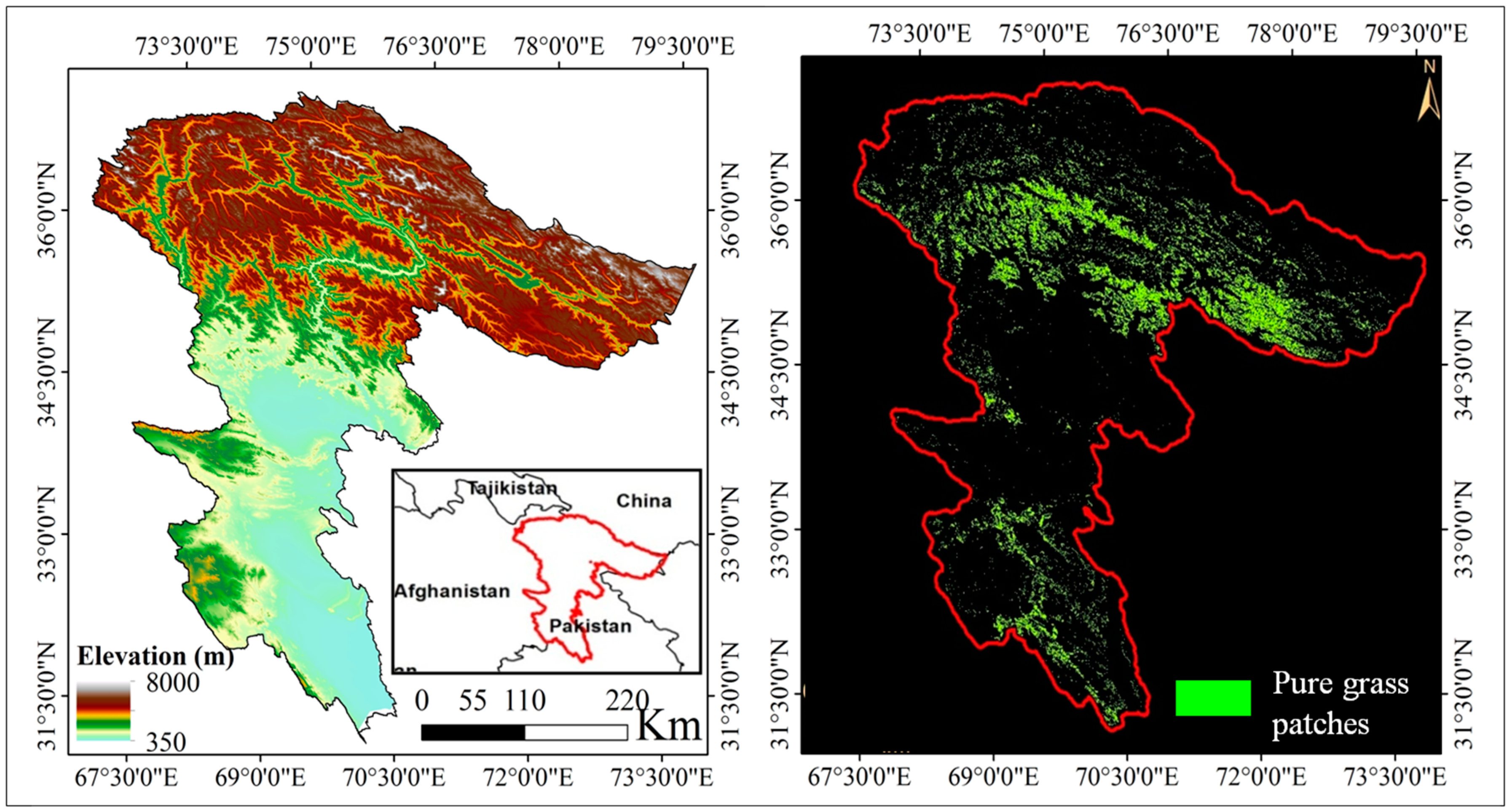
2.1. Study Area

The Hindu Kush Karakoram area of Pakistan covers approximately 17.5 million ha extending across the Khyber Pakhtunkhwa (KP) and Gilgit-Baltistan (GB) provinces in Pakistan approximately between 31° and 37°N and 69° and 78°E (Figure 1). The area has a diverse topography, with alluvial plains, low hills, and high mountains, and elevations that range from approximately 300 to 8000 m (Figure 1). The northern region of the area has a continental steppe climate, with precipitation concentrated in winter and spring [27]. At higher elevations, snowfall is heavier, and large glaciers are prominent features of the landscape.

2.2. Datasets and Data Pre-Processing

In the current study, phenological and productivity patterns were assessed across the ecological zones of the study area by analyzing NDVI time-series data collected from 2001 to 2012 that were acquired by a moderate resolution imaging spectroradiometer (MODIS Terra Satellite; National Aeronautics and Space Administration (NASA); Washington, DC, USA) synthesized at 16-day intervals using maximum value composite algorithm and a 250-m spatial resolution, a standard product coded as MOD13Q1 (Level 3 Product). A total of 276 NDVI 16-day composite images were considered in the analyses. The NDVI product is also accompanied by a quality assessment (QA) layer describing auxiliary information on the quality of the pixels. A reliability index is associated with all pixels, which helps to either exclude or give reduced weight to low-quality pixels when reconstructing the time series. In addition, climate data on rainfall and temperature were used to investigate trends over the 12-year period analyzed in this study. Temperature was estimated using the MOD11C3 moderate resolution imaging spectroradiometer (MODIS MOD11C3; NASA; Washington, D.C., USA) which provides monthly estimates of land surface temperature (LST) with a spatial resolution of 0.05° × 0.05° (~5.6 km at the equator) [28]. LSTs derived from remotely sensed measures have been used previously and are considered as a proxy for air temperature (Ta) [28]. Recent studies have confirmed that LST is highly correlated with air temperature and can be used to linearly estimate daily maximum and minimum air temperatures [29,30]. Rainfall estimates were obtained from a monthly global product (3B43) of the Tropical Rainfall Measuring Mission (TRMM) spanning from 50°N to 50°S at a spatial resolution of 0.25° × 0.25° (~28 km), which provides a monthly average precipitation rate (mm/h) [28]. The monthly average was converted into monthly accumulated rainfall (mm) by multiplying the hourly rate with the total hours in the month [31].

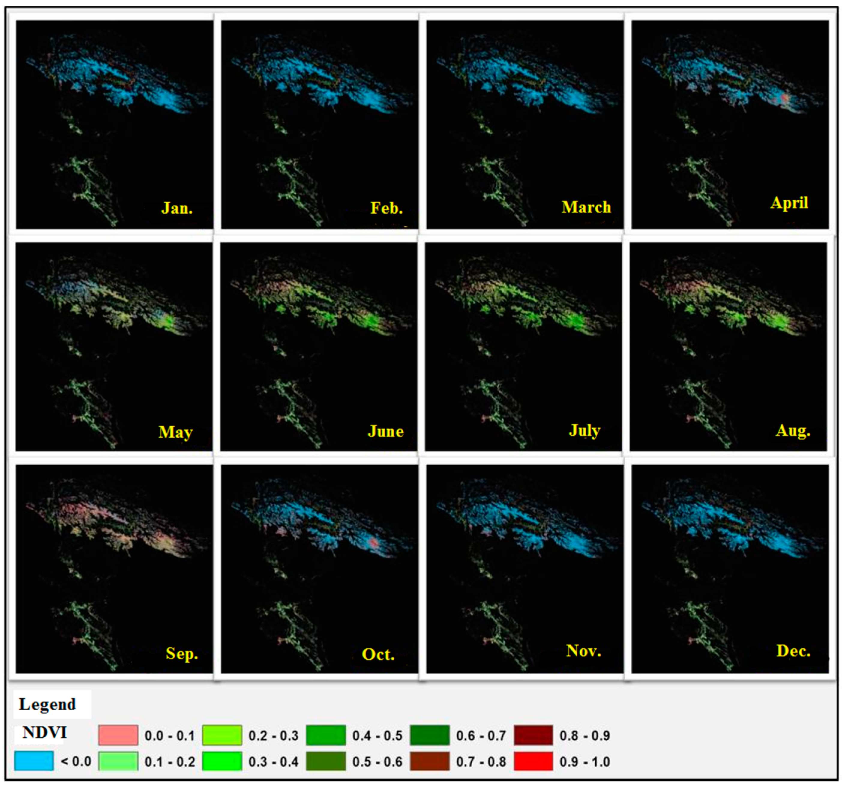
2.2.1. Reconstruction of NDVI Time-Series

NDVI data almost always include disturbances caused by cloud contamination, atmospheric variability, and bidirectional effects [32]. These disturbances appear as undesirable noise and affect the monitoring of land cover and ecosystems [33]. The NDVI product is accompanied by a quality assessment (QA) layer containing auxiliary information on the quality of the pixels, which enables pixels to be excluded or weighted when reconstructing the time series information. A “double logistic regression” approach was used to reconstruct a continuous NDVI time-series for the phenological analysis of the vegetation [34,35,36,37]. This is a well-established method and is particularly suited to the phenological monitoring of rangelands or grasslands from time-series remote-sensing data [36].

The NDVI time-series described by the double logistic function is explained by the following equation (adapted from [37]):

$$NDV{I}_t=NDV{I}_{min}+NDV{I}_d(\frac{1}{1+e^{L_m\left(t-L\right)}}+\frac{1}{1+e^{R_m\left(t-R\right)}}-1)$$

(1)

• NDVI_t = NDVI of the pixel at day of the year (DOY).
• NDVI_min = Minimum NDVI of the NDVI trajectory during the year (lower asymptote).
• NDVI_d = Difference between minimum and maximum (lower and upper asymptote) of the NDVI trajectory during the year.
• $L$ = Position of the left inflection point (change of concavity), point (DOY) where the slope of the function has a maximum change (maximum rate of increase in NDVI) in spring at the start of the season.
• $R$ = Position of the right inflection point (change of concavity), point (DOY) where the slope of the function has a maximum change (maximum rate of decrease in NDVI) in autumn.
• $L_m$ = Maximum slope of the curve at the left inflection point, maximum rate of increase in NDVI
• $R_m$ = Maximum slope of the curve at the right inflection point, maximum rate of decrease in NDVI.

2.2.2. Grassland Mask

A preliminary analysis of the available land-cover maps [38,39] showed that grasslands were not identified separately and they were merged with shrublands. The lack of pure grassland patches meant that it was first necessary to prepare a grassland mask with minimum commission errors so that variations in grasslands could be analyzed [40]. Phenology metrics were generated using a combination of derivative [36] and threshold [41] methods. A rule-based exclusion approach based on a combination of mean vegetation growth metrics (phenology), a digital elevation model (DEM), in situ information, and the land-cover map were used to identify grassland patches with no or a minimum of mixing with other land-cover types. The following steps were followed to prepare the grassland mask for the study:

• Pixels with weak NDVI values (<0.05) were excluded.
• Pixel that were already classified as non-rangelands, such as forests, snow/glaciers, cultivated areas, water, bare lands and urban areas, were removed.
• At higher elevations, because of the prolonged length of the season along with the high productivity and lower maximum seasonal NDVI, the decision was made to mask out evergreen scrub forests (the decision rule was made based on several observations of Google Earth images.
• At mid altitudes in forest zones, forested areas were identified and eliminated based on the extended seasonal length and high NDVI values throughout the year.
• Noisy pixels were further filtered and excluded using a histogram analysis of vegetation phenology based on factors such as a very late start of the growing season (SGST > 230).

2.3. Evaluation of Productivity Metrics

Time-series analyses of NDVI datasets have been extensively used to determine growing season dynamics and productivity patterns [24]. This study used a combination of derivative [36] and threshold [41] methods. First, the NDVI values describing the maximum rates of increase and decrease of mean annual values over the 12 years were calculated. Initially, NDVI values describing the rates of maximum increase and maximum decrease in 12 years’ mean annual NDVI trajectory were computed. Then these NDVI values were used as thresholds in determining the following annual timing metrics of vegetation growth: start and end of growing season, the growing season length (GSL), seasonal cumulative NDVI (SCN) and seasonal maximum NDVI (SMN) (

Table 1. Productivity metrics used in the study.

PPM	Description	Ecological Meaning
Growing season length (GSL)	Number of days between start and end of growing season	Number of days when forage is available
Seasonal cumulative NDVI * (SCN)	Cumulative positive NDVI values of the season	Proxy for seasonal primary production of vegetation
Seasonal maximum NDVI * (SMN)	Maximum NDVI value of the season	Proxy for maximum forage biomass during the season

* NDVI: normalized difference vegetation index.

). Start of growing season is the time when the NDVI value of the season matches the NDVI value at the time T corresponding to the point where the 2nd order derivative of the function is maximum before the maximum NDVI value of the season on the 12 year’s mean trajectory of double logistic fit. End of growing season is the time when the NDVI value of the season matches with the NDVI value defined by the time when NDVI drops to the 80% of the difference between seasonal maximum NDVI and minimum NDVI (NDVI min) on the 12 year’s mean trajectory of double logistic fit. Timing metrics derived through this method correspond to the specific vegetation development stage and further reduce non-climate effects such as aerosols, clouds, disturbances, and defoliation on annual values. The length of the growing season was calculated as the difference between the start of the growing season and its end; SCN is the sum of all NDVI values during the growing season, and SMN is the maximum NDVI value during the growing season. The selected metrics were chosen to reveal the spatiotemporal patterns of grassland productivity.

2.4. Rangeland Growth Trends

Greening or browning trends in the vegetation were assessed using the seasonal nonparametric Mann-Kendal (MK) test [42] because the NDVI dataset violates the assumption of independent Y-values, which is the basis for a linear regression. The MK test can be used with missing or tied data, and its validity does not depend on the data being normally distributed [43]. Positive values indicate increase, negative show decrease, 0 = no change. Once calculated for the whole time-series, if the total number of negative values is more, the trend is negative or vice versa. Essentially, MK indicates the relative frequency of increases minus the relative frequency of decreases. To measure the significance of the trend, a probability index (p-values) is calculated from Z-scores (a standard score to indicate deviations above or below the population mean), giving a value between 0 (highly significant) and 1 (not significant).

2.5. Ecological Zones and Analysis

The high spatial variability that characterizes mountain areas suggests that regional studies should include a microclimatic component, which can be defined by proxy variables such as altitude, slope, and aspect [44]. Altitude was taken as a proxy for a micro-ecological zone to further minimize the effect of spatial variance; the altitudinal gradient was stratified into 10 classes at 500-m intervals of elevation, ranging from <500 to >4500 masl.

Table 2. Ecological zones of the study area.

Ecological Zone	Description	Elevation (masl)	Elevation Range (masl)
Humid sub-tropical zone (HSZ)	Winter pastures. Grasses and forbs along with the green leaves from species such as Olea ferruginea, Grewia optiva, Acacia modesta and Prosopis sp.	300–1000	Range 1 (<500)
			Range 2 (500–1000)
Moist temperate zone (TZ)	Grazing staging areas. Predominantly forest zones with forage areas for livestock grazing during the summer growing season	1000–3000	Range 3 (1000–1500)
			Range 4 (1500–2000)
			Range 5 (2000–2500)
			Range 6 (2500–3000)
Sub-alpine zone (SAZ)	Dominated primarily by Kobersia sp. turf. Sibbaldia cuneata, Trifolium sp. and Poa pratensis are also dominant at various sites	3000–4000	Range 7 (3000–3500)
			Range 8 (3500–4000)
Alpine zone (AZ)	Short summer grazing, dominated by Festuca, Poa, Lolium, Eragrostis, Danthonia, and Phleum, as well as many forbs, such as Primula, Aremons, Fritillaria, and Gentiana sp.	>4000	Range 9 (4000–4500)
			Range 10 (>4500)

summarizes the main features of the four ecological zones that were identified and the grassland classes (vegetation communities) associated with them. The variability in the productivity metrics within each elevation zone in terms of both space and time was taken as a measure representing the heterogeneity within each zone. The spatial variability of a metric within an elevation zone may result from a range of biotic and abiotic gradients and the associated responses in grassland systems; a high spatial variability represents the diversity of habitat conditions. Temporal variability (over the 12 years) represents how the system is experiencing changes over time; a high temporal variability indicates a high sensitivity of the system.

3. Results

Gap-filling of NDVI time-series data produced a cleaned (smoothed), continuous curve of the NDVI for each pixel, while keeping much of the temporal information of the original dataset intact. Spatial and temporal variations of the mean annual grassland growth cycle of the study area over the 12 years from 2001 and 2012 is depicted through representative observations for each month. The spatio-temporal distribution of mean monthly variation of NDVI over 12 years of grasslands along altitudinal and/or latitudinal gradients is presented in Figure 2. The NDVI climatological analysis produced from monthly sequences of NDVI images indicate the spatiotemporal dynamics of grassland distribution at the landscape scale. In winter, most grasslands at higher altitudes (>2500 m) had negative NDVI values due to persistent snow cover; however, these permafrost layers of snow are a critical component for moisture supply to grasses. Several patches at middle and lower elevations did maintain slightly positive NDVI values. Initial increases in NDVI values were usually sharp and probably reflect the combined effects of new vegetation growth and snow melt, which by itself causes an increase in NDVI signals [19,45]. By mid-summer, most of the grasslands displayed rising NDVI values, though a few scattered low elevation patches had already peaked by early summer. Most of the patches were at their peak greenness in mid-summer (approximately June/July), after which NDVI values in most patches slowly decreased in September/October. Sharp decreases in NDVI values were marked by the beginning of winter, the end of the growing season, and the start of the snowy season (October/November) at high elevations.

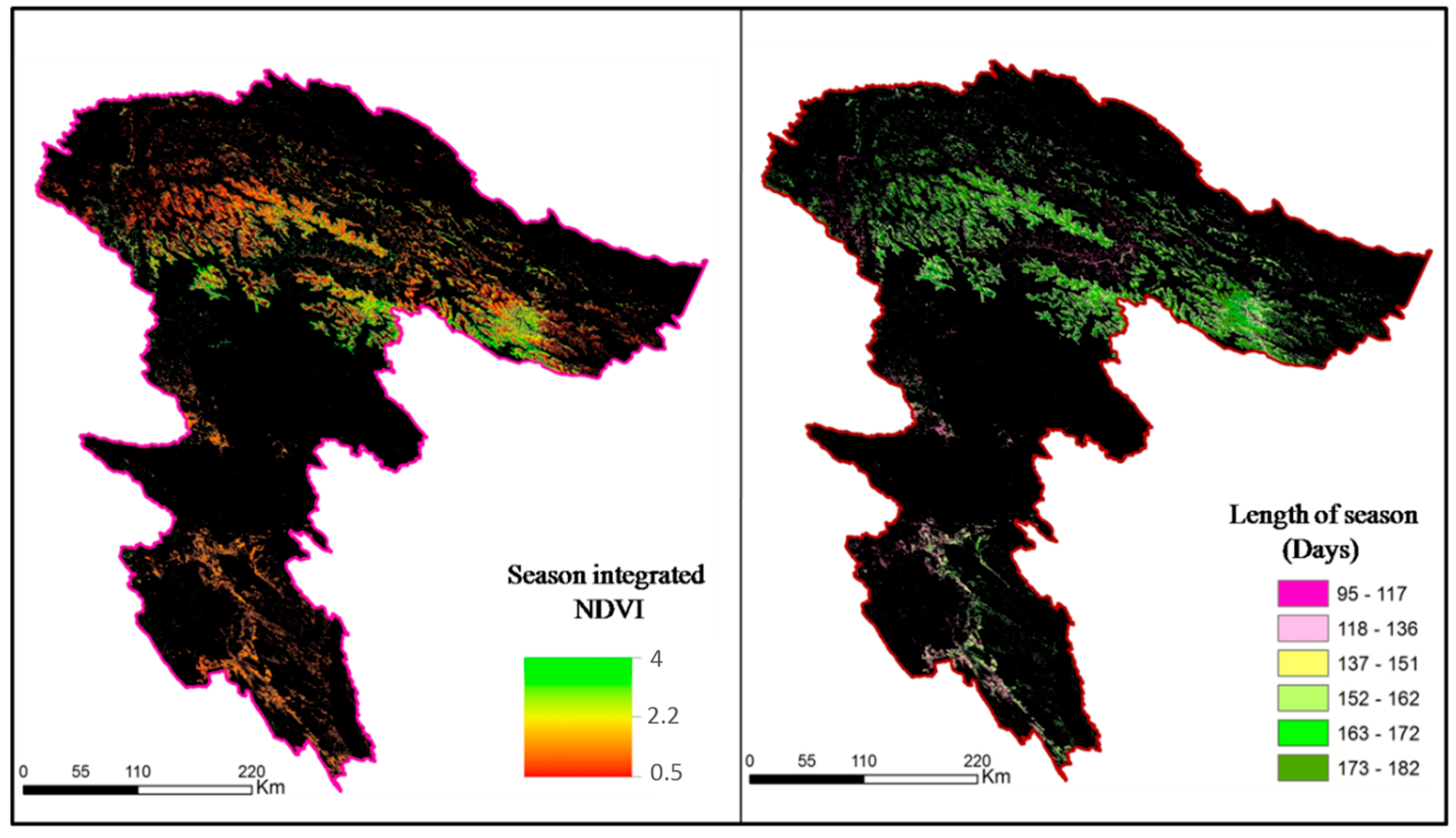
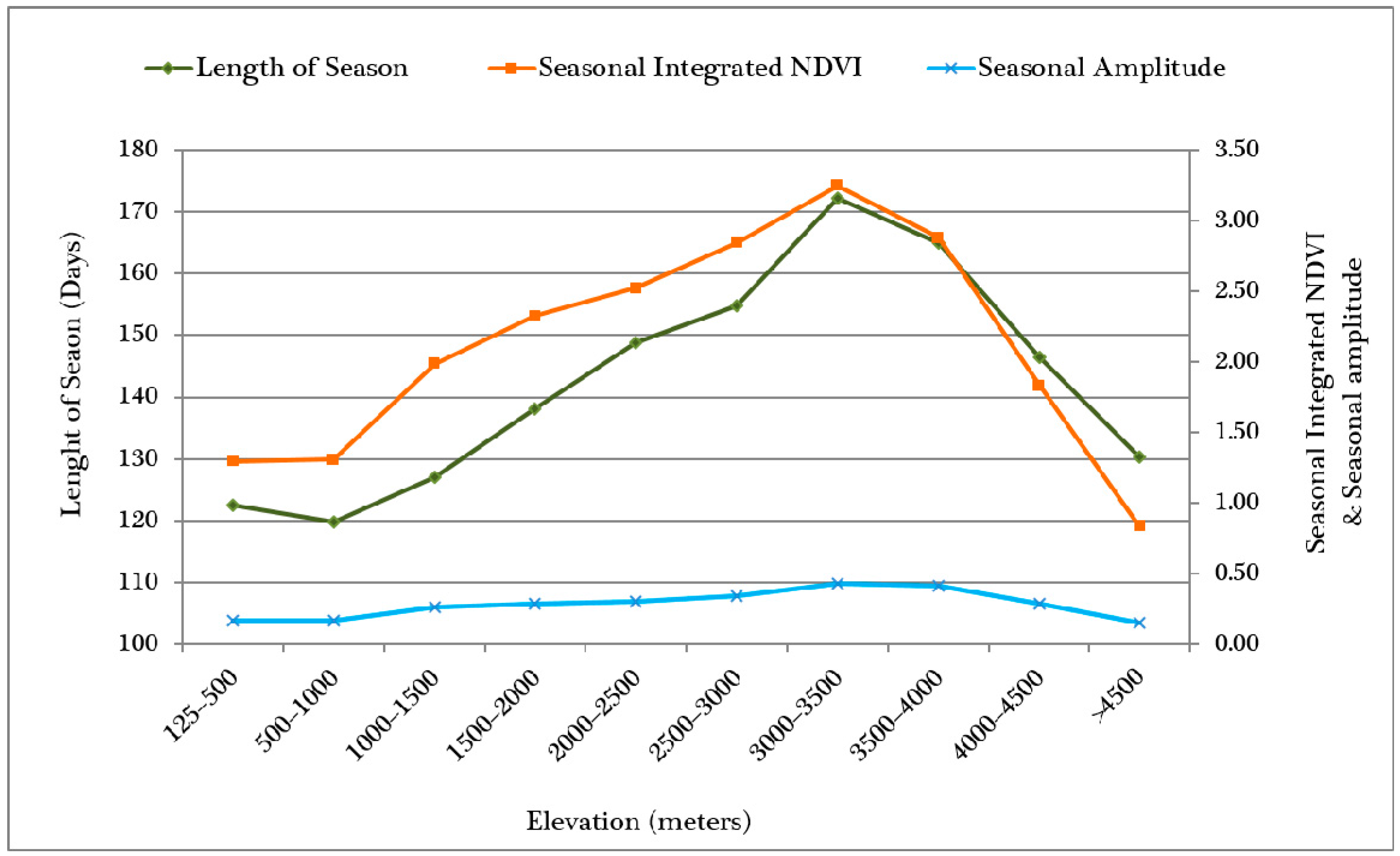
3.1. Rangeland Productivity Patterns

The 12-year means of the productivity metrics were analyzed across the four major ecological zones in the area. Figure 3 shows grassland productivity, as indicated by the SCN values along with the length of the growing season in the respective zones. Overall, in terms of ecological zones, the humid sub-tropical zones (>1000 m) had the shortest seasons and lowest productivity; moist temperate zones (1000–3000 m) had short growing seasons with low productivity; sub-alpine (3000–4000 m) zones had the longest growing seasons and a high growth amplitude, resulting in the highest productivity (SCN); and the alpine zones (<4000 m) has a short growing season with low productivity (Figure 3 and Figure 4).

Vegetation productivity metrics strongly correlated with elevation. The productivity positively related with increased elevation, reach a maximum productivity at an altitude of 3500 m, after which the relation tended to be strongly negative, with productivity sharply dropping to a minimum productivity across the whole range at the highest elevations. The gradual increase in cumulative seasonal productivity along with increased elevation might be a function of the corresponding increase in the length of the growing season.

The spatial and temporal variability in SMN was analyzed to assess the diversity and sensitivity of grasslands across the ecological zones of the area. The alpine and sub-alpine zones had a high spatial variability in SMN. The grasslands in the humid sub-tropical zone were found to have the lowest spatial variability. In contrast, the alpine and sub-alpine zones had a low temporal variability, reflecting a stable system in comparison to the humid sub-tropical zones, which had a high temporal variability. SCN, which is a function of the length of the season and is dictated by climatic conditions and intermediate NDVI values, showed low spatial and temporal variability in the humid sub-tropical zone and at the highest elevations of the alpine zone. Only temporal variability was high in the sub-alpine zone, whereas spatial variability was high in the temperate, sub-alpine, and lower elevations of the alpine zone (

Table 3. A comparison of basic descriptive statistic of productivity metrics over 12 year period (2001–2012) among different zones.

Zone	Elevation (m)	GSL					SMN					SCN
		Mean	Tmp.Std.	Spt.Std.	Tmp.Cov.	Spt.Cov.	Mean	Tmp.Std.	Spt.Std.	Tmp.Cov.	Spt.Cov.	Mean	Tmp.Std.	Spt.Std.	Tmp.Cov.	Spt.Cov.
HSZ	300–500	122	8.97	10.57	0.07	0.09	0.16	0.022	0.028	0.14	0.17	1.3	0.156	0.19	0.12	0.15
	500–1000	120	9.3	9.99	0.08	0.08	0.17	0.023	0.035	0.14	0.21	1.31	0.149	0.22	0.11	0.17
MTZ	100–1500	127	6.01	27.13	0.05	0.21	0.26	0.017	0.142	0.07	0.27	1.99	0.15	1.05	0.08	0.53
	1500–2000	138	8.65	26.84	0.06	0.19	0.28	0.015	0.134	0.05	0.28	2.32	0.188	1.05	0.08	0.45
	2000–2500	149	8.8	26.3	0.06	0.18	0.3	0.018	0.114	0.06	0.29	2.52	0.21	1.01	0.08	0.4
	2500–3000	155	7.88	27.07	0.05	0.17	0.34	0.018	0.124	0.05	0.3	2.85	0.191	1.07	0.07	0.38
SAZ	3000–3500	172	17.75	21.53	0.1	0.13	0.43	0.016	0.138	0.04	0.34	3.25	0.355	1.07	0.11	0.33
	3500–4000	165	20.65	19.57	0.13	0.12	0.41	0.017	0.148	0.04	0.34	2.88	0.371	1.14	0.13	0.39
AZ	4000–4500	146	19.98	21.98	0.14	0.15	0.29	0.013	0.154	0.05	0.34	1.83	0.256	1.1	0.14	0.6
	>4500	130	17.49	22.7	0.13	0.17	0.15	0.008	0.1	0.05	0.33	0.83	0.13	0.67	0.16	0.8

Tmp: Temporal; Spt: Spatial; Std: Standard deviation; Cov.: Covariance; GSL: Growing Season Length; SMN: Seasonal Maximum NDVI; SCN: Seasonal Cumulative NDVI.

).

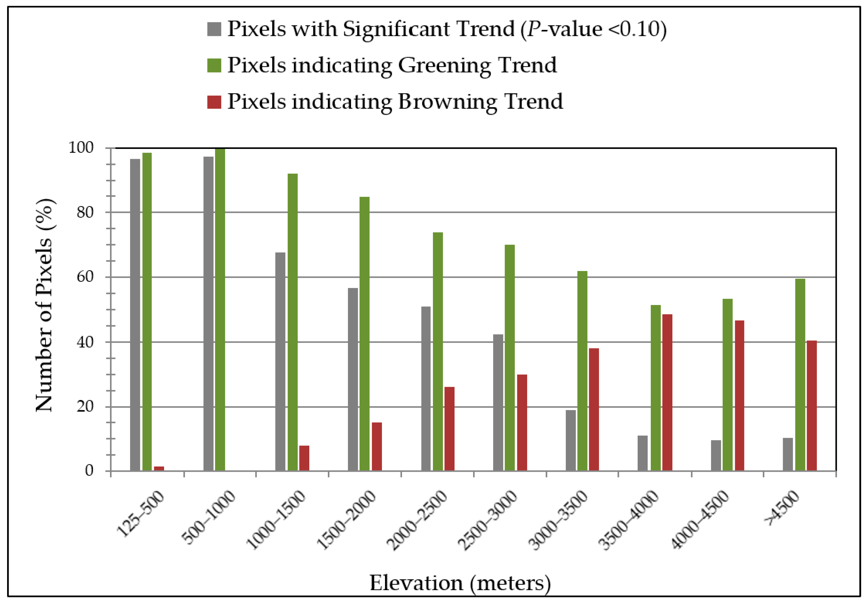
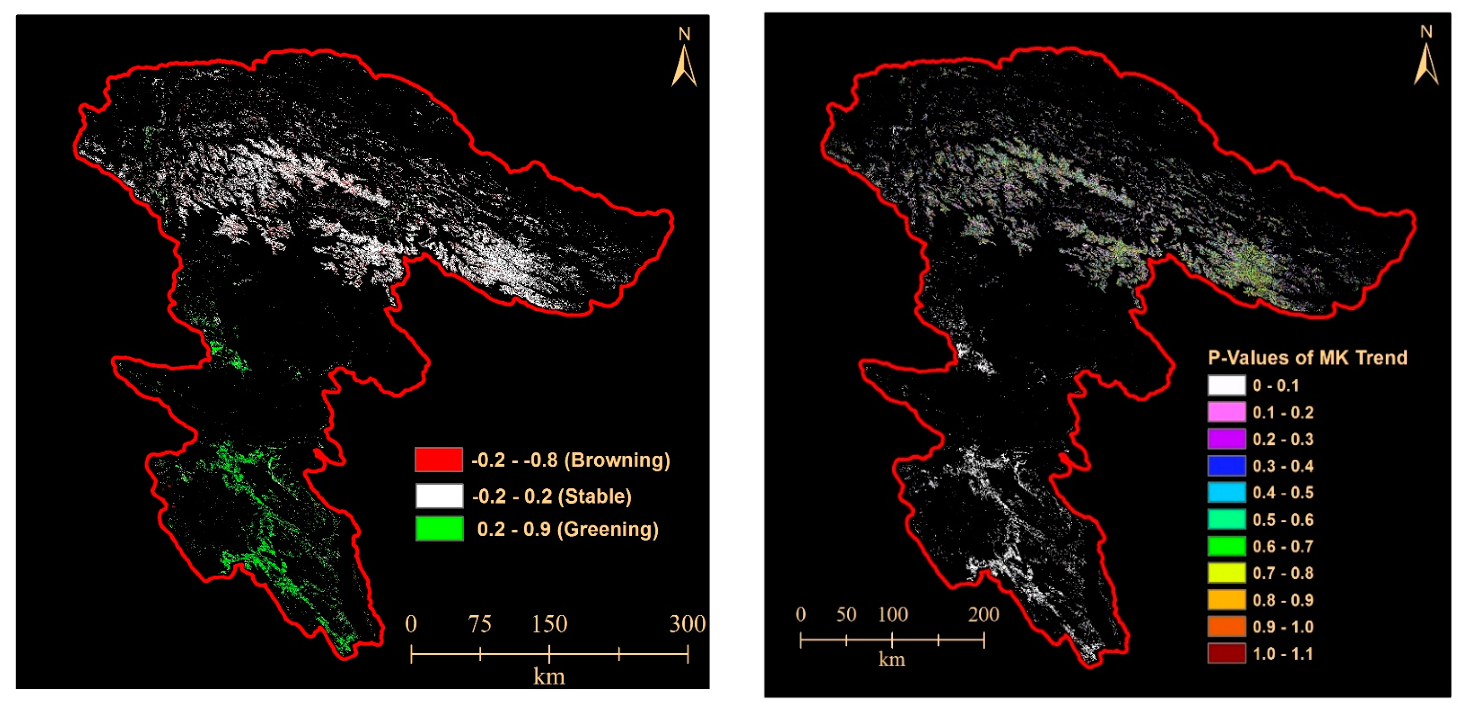
3.2. Greening and Browning Trends

The distribution of greening and browning pixels and the strength of the MK trend with elevation zone are shown in Figure 5 and Figure 6. Overall, 28% of grassland pixels had a significant greening or browning trend (p < 0.1), of which, 84% had a greening trend and 16% a browning trend. The proportion of pixels showing a trend was highest at the lowest altitude (97% in zone 1), and it decreased with increasing altitude (to 10% in zones 9 and 10). The percentage of greening pixels also decreased with altitude, from 99% in zone 1 to 51% in zone 8 (after which it increased slightly). The strength of the trend was also the highest at the lowest altitude (0.43 mean greening pixels in zone 1, and p < 0.001 in 99% of significant pixels), and it decreased with increasing altitude (to 0.15 greening pixels in zone 10).

At mid-elevations (zones 3, 4, 5, and 6), the percentage of pixels and the average strength of the monotonic trend of greening pixels dropped from 92% to 70% and 0.30 to 0.21, respectively, whereas the remaining browning pixels increased in terms of percentage (8% to 30%) and the strength of the trend (−0.20 to −0.25). The high-elevation grasslands (range 7, 8, 9, and 10) seemed be represented by almost equal numbers of greening (59% to 51%) and browning (41% to 49%.) pixels, but the strength and significance of the trends became weaker for both greening (0.17 to 0.15, p-values 0.05) and browning (−0.17 to −0.14, p-values 0.05) pixels.

The greening/browning trends over the 12 years also showed contrasting patterns across the ecological zones. Almost all of the area in humid sub-tropical regions showed a strong and statistically significant greening trend. The majority of temperate regions also showed a greening trend; however, the trend was only statistically significant in half of these areas. When compared with the trends for temperature and rainfall across the ecological zones of the regions (

Table 4. Linear trend in annual rainfall and temperature during growing season period (April–October) derived from the 12 years of data from MODIS lands surface temperature (LST) and Tropical Rainfall Measuring Mission (TRMM) rainfall data.

Ecological Zone	Elevation (m)	Temperature (r)	Rainfall (r)
Humid sub-tropical zone (HSZ)	300–500	−0.22	0.74
	500–1000	−0.29	0.75
Moist temperate zone (TZ)	1000–1500	−0.21	0.53
	1500–2000	−0.20	0.51
	2000–2500	−0.19	0.40
	2500–3000	−0.16	0.32
Sub-alpine zone (SAZ)	3000–3500	−0.05	0.27
	3500–4000	−0.02	0.00
Alpine zone (AZ)	4000–4500	−0.02	0.16
	>4500	−0.02	0.13

) over the 12 years, temperature does not have any clear trend, while rainfall shows a significant increase in the humid sub-tropical regions. Thus, the greening trend in this region can be attributed to increases in rainfall as vegetation growth is mostly limited by moisture in the humid sub-tropical region. In contrast, relatively large areas of alpine and sub-alpine regions showed browning trends.

4. Discussion

Grassland productivity in the Hindu Kush Karakoram region was found to increase with elevation, reaching a maximum in the sub-alpine zone. The high productivity in alpine zone is attributed to both the seasonal amplitude (maximum plant growth/photosynthesis) and the extended length of the growing season in the zone, which is similar to the findings of previous ground-based assessments [14]. The high-mountain pastures in the alpine range provide good forage for livestock during the growing season and therefore represent a very important part of the transhumance system. The greater biomass in the alpine ranges in spring, summer and autumn, compared to biomass in the dry temperate or foothill ranges presumably reflects the increased soil moisture made available from snow melt during spring/early summer, allowing increased plant growth [46,47]. The large area of sub-alpine grasslands with a longer GSL indicates their greater grazing potential. However, a high degree of temporal and spatial variability in the GSL, as observed in this study, cautions for a better ground-based understanding of the causes of variability and the need for associated judicious planning of potential grazing. Our analysis of its production patterns provides valuable information for analyzing the grazing potential of these regions. On the other hand, the humid sub-tropical zones, which occupy the second largest area in the region, have a shorter GSL and require proper planning to meet grazing needs.

The results of the present study are similar to those of global studies. For example, a previous study [20] showed a global trend of 25% greening trend and 3% browning trend across all the vegetated areas of the world, with every vegetation type contributing to greening, but most prominently woody savannah and grasslands. The browning trends in alpine and sub-alpine areas can be attributed to the overgrazing of these areas [14]. Observed that vegetation offtake was significantly higher in sub-alpine regions than in humid sub-tropical and temperate regions due to the high grazing intensity during the entire growing season [20]. Holechek, Pieper and Herbel [48] assessed that grazing area in subalpine and alpine pastures of Kashmir decreased from 0.15 ha/animal in 1977 to 0.10 ha/ animal in 1982 [49] and which continued to further decrease in later years [50]. Saqib and Sultan [51] observed that the most prone areas to such disturbance are the sub-alpine and alpine zones, which are main supply of ethno-botanically important flora. Also, the sub-alpine and alpine pastures showed a closer relationship between NPP and off-take, indicating a greater use of more productive vegetation [51,52]. Sub-alpine pastures are used as winter-spring pastures by nomadic herders, but the sub-tropical belt or lower temperate belt are normally used by sedentary farmers. Grazing pressures are different between low and high altitudes. The lower part of the sub-alpine belt may be used by farmers in summer, so there is an overlap in the use of this belt by sedentary farmers and nomadic herders. Therefore, this ecosystem interface experiences more grazing pressure than other belts. The fact that the sub-alpine grasslands have the highest productivity (SCN) and a high degree of spatial variability in the seasonal maximum NDVI (reflecting heterogeneous grasslands) indicates the high value of this region, while at the same time, the relatively high browning trends indicate the ongoing degradation in these pristine rangelands. Thus special attention is needed for the sustainable management of rangelands in the sub-alpine zones of the Hindu Kush Karakoram region.

5. Conclusions

This study provides an overview of grasslands conditions in a large landscape dominating by rangelands. The assessment suggests that within the spatial landscape, vegetation productivity increases with elevation and sub-alpine zones has significantly high productivity. The high productivity is attributed to seasonal amplitude as well as extended length of season in the zone. The study indicated the signs of degradation in the sub-alpine zone which is significantly important for transhumance grazing system in the area. Spatial information on grassland productivity is potentially useful for spatial planning of grazing routes within each range and regulating land use across the range to sustainably meet the grazing needs of the nomadic herds. The information derived from this study can be used to support informed decision making for long-term grazing management.

In the rangelands studies, which involve vast areas, remote sensing methods can provide a reliable overview on the vegetation conditions. However, linking remotely sensed data with site-based understanding is required to address complex ecological questions across a range of spatial scales. This is a subject that would merit more attention in future works.

References

1. Breman, H.; de Wit, C.T. Rangeland productivity and exploitation in the sahel. Science 1983, 221, 1341–1347. [Google Scholar] [CrossRef] [PubMed]
2. Vetter, S. Rangelands at equilibrium and non-equilibrium: Recent developments in the debate. J. Arid Environ. 2005, 62, 321–341. [Google Scholar] [CrossRef]
3. Ellis, J.E.; Swift, D.M. Stability of African Pastoral Ecosystems: Alternate Paradigms and Implications for Development. J. Range Manag. 1988, 41, 450–459. [Google Scholar] [CrossRef]
4. Illius, A.W.; O’Connor, T.G. On the relevance of nonequilibrium concepts to arid and semiarid grazing systems. Ecol. Appl. 1999, 9, 798–813. [Google Scholar] [CrossRef]
5. Joshi, L.; Shrestha, R.M.; Jasra, A.W.; Joshi, S.; Gilani, H.; Ismail, M. Rangeland ecosystem services in the Hindu Kush Himalayan Region. In High-Altitude Rangelands and Their Interfaces in the Hindu Kush Himalayas; Ning, W., Rawat, G.S., Joshi, S., Ismail, M., Sharma, E., Eds.; The International Centre for Integrated Mountain Development (ICIMOD): Kathmandu, Nepal, 2013; pp. 157–174. [Google Scholar]
6. Mansouri Daneshvar, M.R.; Bagherzadeh, A.; Khosravi, M. Assessment of drought hazard impact on wheat cultivation using standardized precipitation index in Iran. Arab. J. Geosci. 2012, 6, 4463–4473. [Google Scholar] [CrossRef]
7. Beniston, M. Climatic change in mountain regions: A review of possible impacts. Clim. Chang. 2003, 59, 5–31. [Google Scholar] [CrossRef]
8. Nüsser, M.; Clemens, J. Impacts on Mixed Mountain Agriculture in the Rupal Valley, Nanga Parbat, Northern Pakistan. Mt. Res. Dev. 1996, 16, 117–133. [Google Scholar] [CrossRef]
9. Kreutzmann, H. Pastoral Practices and their Transformation in the North-Western Karakoram. Nomadic Peoples 2004, 8, 54–88. [Google Scholar] [CrossRef]
10. Rahman, A.; Duncan, A.J.; Miller, D.W.; Clemens, J.; Frutos, P.; Gordon, I.J.; Rehman, A.U.R.; Baig, A.; Ali, F.; Wright, I.A. Livestock feed resources, production and management in the agro-pastoral system of the Hindu Kush-Karakoram-Himalayan region of Pakistan: The effect of accessibility. Agric. Syst. 2008, 96, 26–36. [Google Scholar] [CrossRef]
11. Eklundh, L.; Olsson, L. Vegetation index trends for the African Sahel 1982–1999. Geophys. Res. Lett. 2003, 30, 1430. [Google Scholar] [CrossRef]
12. Tadesse, T.; Brown, J.F.; Hayes, M.J. A new approach for predicting drought-related vegetation stress: Integrating satellite, climate, and biophysical data over the US central plains. ISPRS J. Photogramm. Remote Sens. 2005, 59, 244–253. [Google Scholar] [CrossRef]
13. Liu, L.; Liu, L.; Liang, L.; Donnelly, A.; Park, I.; Schwartz, M.D. Effects of elevation on spring phenological sensitivity to temperature in Tibetan Plateau grasslands. Chinese Sci. Bull. 2014, 59, 4856–4863. [Google Scholar] [CrossRef]
14. Omer, R.M.; Hester, A.J.; Gordon, I.J.; Swaine, M.D.; Raffique, S.M. Seasonal changes in pasture biomass, production and offtake under the transhumance system in northern Pakistan. J. Arid Environ. 2006, 67, 641–660. [Google Scholar] [CrossRef]
15. Tucker, C.J.; Sellers, P.J. Satellite remote sensing of primary production. Int. J. Remote Sens. 1986, 7, 1395–1416. [Google Scholar] [CrossRef]
16. Rigge, M.; Smart, A.; Wylie, B.; Gilmanov, T.; Johnson, P. Linking Phenology and Biomass Productivity in South Dakota Mixed-Grass Prairie. Rangel. Ecol. Manag. 2013, 66, 579–587. [Google Scholar] [CrossRef]
17. Pettorelli, N.; Vik, J.O.; Mysterud, A.; Gaillard, J.-M.; Tucker, C.J.; Stenseth, N.C. Using the satellite-derived NDVI to assess ecological responses to environmental change. Trends Ecol. Evol. 2005, 20, 503–510. [Google Scholar] [CrossRef] [PubMed]
18. Huete, A.; Didan, K.; Miura, T.; Rodriguez, E.; Gao, X.; Ferreira, L. Overview of the radiometric and biophysical performance of the MODIS vegetation indices. Remote Sens. Environ. 2002, 83, 195–213. [Google Scholar] [CrossRef]
19. Thein, T.R.; Watson, F.G.R.; Cornish, S.S.; Anderson, T.N.; Newman, W.B.; Lockwood, R.E. Vegetation Dynamics of Yellowstone’s Grazing System. Terr. Ecol. 2008, 3, 113–133. [Google Scholar]
20. Zhu, Z.; Bi, J.; Pan, Y.; Ganguly, S.; Anav, A.; Xu, L.; Samanta, A.; Piao, S.; Nemani, R.; Myneni, R. Global Data Sets of Vegetation Leaf Area Index (LAI)3g and Fraction of Photosynthetically Active Radiation (FPAR)3g Derived from Global Inventory Modeling and Mapping Studies (GIMMS) Normalized Difference Vegetation Index (NDVI3g) for the Period 1981 to 2011. Remote Sens. 2013, 5, 927–948. [Google Scholar]
21. Fensholt, R.; Sandholt, I.; Rasmussen, M.S. Evaluation of MODIS LAI, fAPAR and the relation between fAPAR and NDVI in a semi-arid environment using in situ measurements. Remote Sens. Environ. 2004, 91, 490–507. [Google Scholar] [CrossRef]
22. Wang, J.; Rich, P.M.; Price, K.P.; Kettle, W.D. Relations between NDVI and tree productivity in the central Great Plains. Int. J. Remote Sens. 2004, 25, 3127–3138. [Google Scholar] [CrossRef]
23. Bradley, B.A.; Jacob, R.W.; Hermance, J.F.; Mustard, J.F. A curve fitting procedure to derive inter-annual phenologies from time series of noisy satellite NDVI data. Remote Sens. Environ. 2007, 106, 137–145. [Google Scholar] [CrossRef]
24. Xu, L.; Myneni, R.B.; Chapin, F.S., III; Callaghan, T.V.; Pinzon, J.E.; Tucker, C.J.; Zhu, Z.; Bi, J.; Ciais, P.; Tømmervik, H.; et al. Temperature and vegetation seasonality diminishment over northern lands. Nat. Clim. Chang. 2013, 3, 581–586. [Google Scholar] [CrossRef]
25. Nemani, R.R.; Keeling, C.D.; Hashimoto, H.; Jolly, W.M.; Piper, S.C.; Tucker, C.J.; Myneni, R.B.; Running, S.W. Climate-driven increases in global terrestrial net primary production from 1982 to 1999. Science 2003, 300, 1560–1563. [Google Scholar] [CrossRef] [PubMed]
26. Potter, C.S.; Klooster, S.; Brooks, V. Interannual Variability in Terrestrial Net Primary Production: Exploration of Trends and Controls on Regional to Global Scales. Ecosystems 1999, 2, 36–48. [Google Scholar] [CrossRef]
27. Archer, D.R.; Fowler, H.J. Spatial and temporal variations in precipitation in the Upper Indus Basin, global teleconnections and hydrological implications. Hydrol. Earth Syst. Sci. 2004, 8, 47–61. [Google Scholar] [CrossRef]
28. Rhee, J.; Im, J.; Carbone, G.J.; Jensen, J.R. Delineation of climate regions using in-situ and remotely-sensed data for the Carolinas. Remote Sens. Environ. 2008, 112, 3099–3111. [Google Scholar] [CrossRef]
29. Vancutsem, C.; Ceccato, P.; Dinku, T.; Connor, S.J. Evaluation of MODIS land surface temperature data to estimate air temperature in different ecosystems over Africa. Remote Sens. Environ. 2010, 114, 449–465. [Google Scholar] [CrossRef]
30. Schwarz, N.; Schlink, U.; Franck, U.; Großmann, K. Relationship of land surface and air temperatures and its implications for quantifying urban heat island indicators—An application for the city of Leipzig (Germany). Ecol. Indic. 2012, 18, 693–704. [Google Scholar] [CrossRef]
31. Immerzeel, W.W.; Droogers, P.; de Jong, S.M.; Bierkens, M.F.P. Large-scale monitoring of snow cover and runoff simulation in Himalayan river basins using remote sensing. Remote Sens. Environ. 2009, 113, 40–49. [Google Scholar] [CrossRef]
32. Fernandes, J.L.; Rocha, J.V.; Augusto, R.; Lamparelli, C. Sugarcane yield estimates using time series analysis of spot vegetation images temporais de imagens spot vegetation. Distribution 2011, 68, 139–146. [Google Scholar]
33. Chen, J.; Jönsson, P.; Tamura, M.; Gu, Z.; Matsushita, B.; Eklundh, L. A simple method for reconstructing a high-quality NDVI time-series data set based on the Savitzky–Golay filter. Remote Sens. Environ. 2004, 91, 332–344. [Google Scholar] [CrossRef]
34. Fisher, J.; Mustard, J.; Vadeboncoeur, M. Green leaf phenology at Landsat resolution: Scaling from the field to the satellite. Remote Sens. Environ. 2006, 100, 265–279. [Google Scholar] [CrossRef]
35. Heumann, B.W.; Seaquist, J.W.; Eklundh, L.; Jönsson, P. AVHRR derived phenological change in the Sahel and Soudan, Africa, 1982–2005. Remote Sens. Environ. 2007, 108, 385–392. [Google Scholar] [CrossRef]
36. Butt, B.; Turner, M.D.; Singh, A.; Brottem, L. Use of MODIS NDVI to evaluate changing latitudinal gradients of rangeland phenology in Sudano-Sahelian West Africa. Remote Sens. Environ. 2011, 115, 3367–3376. [Google Scholar] [CrossRef]
37. Busetto, L.; Colombo, R.; Migliavacca, M.; Cremonese, E.; Meroni, M.; Galvagno, M.; Rossini, M.; Siniscalco, C.; Morra Di Cella, U.; Pari, E. Remote sensing of larch phenological cycle and analysis of relationships with climate in the Alpine region. Glob. Chang. Biol. 2010, 16, 2504–2517. [Google Scholar] [CrossRef]
38. Shehzad, K.; Qamer, F.M.; Murthy, M.S.R.; Abbas, S.; Bhatta, L.D. Deforestation trends and spatial modelling of its drivers in the dry temperate forests of northern Pakistan—A case study of Chitral. J. Mt. Sci. 2014, 11, 1192–1207. [Google Scholar] [CrossRef]
39. Chen, J.; Chen, J.; Liao, A.; Cao, X.; Chen, L.; Chen, X.; He, C.; Han, G.; Peng, S.; Lu, M.; et al. Global Land Cover Mapping at 30 m Resolution: A POK-Based Operational Approach. ISPRS J. Photogramm. Remote Sens. 2014, 103, 7–27. [Google Scholar] [CrossRef]
40. Vrieling, A.; Beurs, K.M.; Brown, M.E. Variability of African farming systems from phenological analysis of NDVI time series. Clim. Change. 2011, 109, 455–477. [Google Scholar] [CrossRef]
41. Shrestha, U.B.; Gautam, S.; Bawa, K.S. Widespread climate change in the Himalayas and associated changes in local ecosystems. PLoS ONE 2012, 7, e36741. [Google Scholar] [CrossRef] [PubMed]
42. Meng, M.; Ni, J.; Zong, M. Impacts of changes in climate variability on regional vegetation in China: NDVI-based analysis from 1982 to 2000. Ecol. Res. 2011, 26, 421–428. [Google Scholar] [CrossRef]
43. De Jong, R.; de Bruin, S.; de Wit, A.; Schaepman, M.E.; Dent, D.L. Analysis of monotonic greening and browning trends from global NDVI time-series. Remote Sens. Environ. 2011, 115, 692–702. [Google Scholar] [CrossRef] [Green Version]
44. Kariyeva, J.; van Leeuwen, W.J.D. Environmental Drivers of NDVI-Based Vegetation Phenology in Central Asia. Remote Sens. 2011, 3, 203–246. [Google Scholar] [CrossRef]
45. Reed, B.; Brown, J. Measuring phenological variability from satellite imagery. J. Veg. Sci. 1994, 5, 703–714. [Google Scholar] [CrossRef]
46. Seth, C.M. Biomass fluctuation in alpine pastures of Kashmir Himalaya. Ann. Arid Zone 1996, 35, 65–67. [Google Scholar]
47. Sardar, M.R. Indigenous Production and Utilization Systems in the High Altitude Alpine Pasture, Saif-Ul-Maluk (NWFP), Pakistan.; FAO and Pakistan Forest Institute: Peshawar, Pakistan, 1997. [Google Scholar]
48. Holechek, J.L.; Pieper, R.D.; Herbel, C.H. Range Management, Principles and Practices, 3rd ed.; Prentice-Hall: Upper Saddle River, NJ, USA, 1998. [Google Scholar]
49. Misri, B. Improvement of Sub-alpine and Alpine Himalayan Pastures, 2013. Food and Agriculture Organization of the United Nations. Available online: http://www.fao.org/ag/AGP/AGPC/doc/pasture/peshawarproceedings/improvementsubalpine.pdf (accessed on 14 September 2016).
50. Qureshi, R.A.; Gilani, S.A.; Ashraf, M. Ethnobotanical studies with special reference to plants phenology at Sudhan Gali and Ganga Chotti Hills (District Bagh, A.K.). Electron. J. Environ. Agric. Food Chem. 2007, 6, 2207–2215. [Google Scholar]
51. Saqib, Z.; Sultan, A. Ethnobotany of Palas Valley, Pakistan. Ethnobot. Leafl. 2005, 1, 28. Available online: http://opensiuc.lib.siu.edu/ebl/vol2005/iss1/28/ (accessed on 14 September 2016). [Google Scholar]
52. Stoddart, L.A.; Smith, A.D.; Box, T.W. Range Management, 3rd ed.; McGraw-Hill Book Company: New York, NY, USA, 1975. [Google Scholar]
Figure 1. Map of study area showing the topography and grass-dominated rangelands (Projection: Geographic, WGS84).
Sustainability 08 00961 g001
Figure 2. The 12 years’ mean monthly variation of normalized difference vegetation index (NDVI).
Sustainability 08 00961 g002
Figure 3. Patterns in grassland productivity (season cumulative NDVI) and length of season across the study area.
Sustainability 08 00961 g003
Figure 4. Patterns in grassland productivity and growing season length across the elevation zones.
Sustainability 08 00961 g004
Figure 5. Spatial distribution of greening and browning trends along with respective significance (p-value).
Sustainability 08 00961 g005
Figure 6. Graphical representation of significant greening/browning pixels along elevation zones.
Sustainability 08 00961 g006