Optimization of an Improved Intermodal Transit Model Equipped with Feeder Bus and Railway Systems Using Metaheuristics Approaches

Abstract

One of the serious concerns in network design is creating an efficient and appropriate network capable of efficiently migrating the passenger’s mode of transportation from private to public. The main goal of this study is to present an improved model for combining the feeder bus network design system and the railway transit system while minimizing total cost. In this study, the imperialist competitive algorithm (ICA) and the water cycle algorithm (WCA) were employed to optimize feeder bus and railway services. The case study and input data were based on a real transit network in Petaling Jaya, Kuala Lumpur, Malaysia. Numerical results for the proposed model, including the optimal solution, statistical optimization results and the convergence rate, as well as comparisons are discussed in detail.

1. Introduction

Transportation is a multimodal, multi-problem and multi-spectral system, as it involves different categories and activities, such as policy-making, planning, designing, infrastructure construction and development. Currently, considering the significant developments in technology, economy and society, an efficient transportation system plays a key role in passengers’ satisfaction and the reduction of costs.

Many people use public transportation systems to reach their destination; however, others employ personal vehicles. Passengers are more likely to use a transit service that is highly reliable. Travelers may switch to other transportation modes if a transit service does not provide the expected levels of service [1]. To prevent the increase of private transport entering city centers, effective alternative travel modes must be provided [2]. Nuzzolo and Comi [3] investigated methods of transit network modelling that can be implemented in transit decision-making support system tools to improve their performances, according to the latest innovations in information technology and telematics.

In addition, a good public transportation system has been recognized as a potential means of reducing air pollution, decreasing energy consumption, increasing mobility and improving traffic congestion. In order to improve complicated public transportation systems, a well-integrated transit system in urban areas can play a crucial role in passengers’ satisfaction and reduce operating costs. This system usually consists of integrated rail lines and a number of feeder routes connecting transfer stations.

In general, previous approaches to tackle transit network problems can be divided into two major groups: analytic and network approaches. These approaches differ in their purposes and have different advantages and disadvantages. They should be considered as complementary rather than alternative [4]. Numerous studies have attempted to implement analytic models [5,6,7,8,9,10]. On the other hand, some of the researchers adopted network approaches instead of analytical methods [2,11,12,13,14]. Many studies have been carried out to identify solutions using the aforementioned approaches. These can be categorized into four groups, namely mathematical, heuristic, metaheuristic and hybrid techniques [15].

Kuah and Perl [6] presented a mathematical method for designing an optimal feeder bus network to access an existing rail line. Furthermore, Chang and Hsu [10] developed a mathematical model to analyze the passenger waiting time in an intermodal station in which the intercity transit system was served by feeder buses. They presented the analytic model for quantifying the relationships of passenger waiting time to the reliability of feeder bus services and the capacity of intercity transit.

A large number of research papers has been published in recent years utilizing heuristic methods due to their flexibility. Shrivastav and Dhingra [12] developed a heuristic algorithm to integrate suburban stations and bus services, along with the optimization of coordinated schedules for feeder bus services using existing schedules for suburban trains. Sumalee et al. [16] proposed a stochastic network model for a multimodal transport network that considers auto, bus, underground and walking modes. Chowdhury [9] proposed a model for better coordination of the intermodal transit system. Furthermore, Steven and Chien [17] suggested the use of a specific feeder bus service to provide shuttle service between a recreation center and a major public transportation facility. They suggested an integrated methodology (i.e., analytical and numerical techniques) for the development and optimization of decision variables, including bus headway, vehicle size and route choice.

In terms of metaheuristic methods, Kuan [13] applied genetic algorithms (GAs), ant colony optimization (ACO), simulated annealing (SA) and tabu search (TS) to resolve a feeder network design problem (FNDP) for a similar work conducted by Kuah and Perl [11], which improved previously-proposed solutions.

In another study carried out by Shrivastava and O’Mahony [18], optimum feeder routes and schedules for a suburban area were determined using GAs. Mohaymany and Gholami [19] suggested an approach for solving multi-modal FNDP (MFNDP), whose objective was to minimize the total operator, user and society costs. They used ACO for constructing routes and modifying the optimization procedure in order to identify the best mode and route in the service area.

Hybrid methods are categorized as another type of solution method that combines the abilities of different computational techniques to solve complex problems. Shrivastava and O’Mahony [20] developed the Shrivastava–O’Mahony hybrid feeder route generation algorithm (SOHFRGA). The idea was to develop public bus routes and to coordinate schedules in a suburban area.

Numerous researchers have attempted to design a more efficient feeder network and to provide feeder services connecting major transportation systems and welfare facilities. The main target of this paper is to represent an improved model and to present an efficient transit system to increase the efficiency of feeder network designs in order to minimize costs.

The structure of this paper is organized as follows: Section 2 and Section 3 present a brief description and definition of the problem and explain the details of the mathematical model, respectively. Section 4 provides succinct representations of the applied ICA and WCA in order to optimize the transit system problem considered. The computational optimization results obtained from the methods used along with a discussion and comparisons are presented in Section 5. Finally, the concluding results and suggestions for future research are given in Section 6.

2. Problem Definition and Assumptions

In large metropolitan areas, particularly those with high transit demand, an integrated transit system consisting of rail lines and a number of feeder routes connected at different transfer stations is essential. Consequently, designing a proper feeder network that can provide access to an existing rail system and coordinate the schedule of transit service can be a significant issue.

The development of improved integrated intermodal systems can result in a higher quality of service and passenger satisfaction by providing better coverage, reduced access time, minimal delay and shorter travel times. From the transit operators’ point of view, the operating costs may be reduced by an overall coordination between different public transport modes. Profit can also be increased by shorter route maintenance and eliminating the duplication of routes by trains and buses.

This study is focused on designing a set of feeder bus routes and determining operating frequency on each route, such that the objective function of the sum of the operator, user and social cost is minimized. The mathematical formulation of the improved model and the details of the constraints are presented in the following sections.

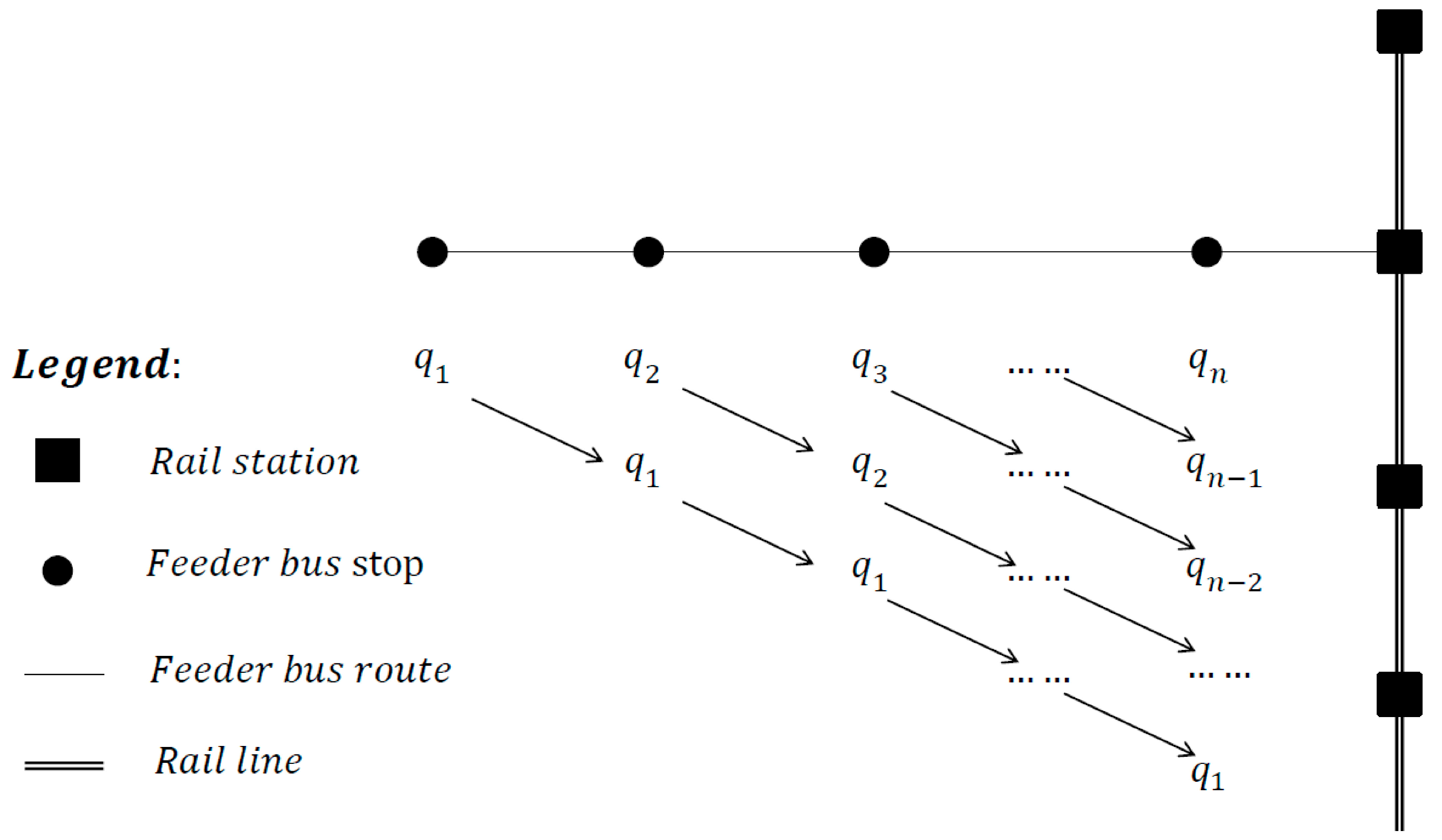
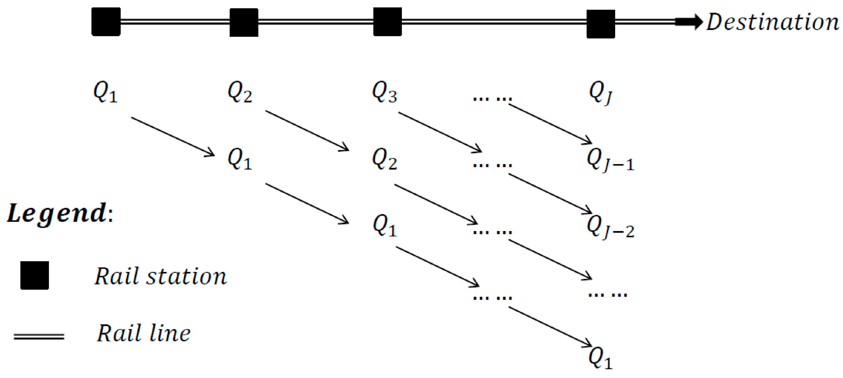
An intermodal transit network consisting of a rail line and feeder bus routes connecting the transfer stations is assumed to serve the examined area. The optimal transit system will be determined based on an assumed route structure (i.e., one rail line and feeder bus routes are linked with straight lines between nodes) and the peak hour demand situations in the entire service area. To formulate the mathematical model for an intermodal transit system and its application in the case study, the following assumptions are made:

(1)

The transit network was designed with feeder buses and a fixed rail line.

(2)

Transit demand is assumed to be independent of the quality of transit service (i.e., fixed demand). The demand pattern for feeder bus routes is many-to-one.

(3)

The location of nodes (i.e., bus stops and rail stations) is given. Some of the model parameters (e.g., vehicle sizes, operating speed, cost) are specified.

(4)

All feeder routes can be used in both directions for the transit service.

3. Model Formulation

To propose a mathematical formulation for the model based on the problem statement of this study, the total cost function is expressed in Equation (1). The total cost function is the sum of the user, operator and social costs, which can be formulated as follows:

C_T = C_u + C_o + C_s

(1)

where C_T, C_u, C_o and C_s represent the total cost, user costs, operation costs and social costs, respectively. The well-structured cost classification for the proposed model is shown in Figure 1.

Table 1. Illustration of the total cost with all terms in the proposed improved model.

Total Cost (CT)
User Cost (Cu) a			Operating Cost (Co) b				Social Cost (Cs) c
Feeder Bus and Train			Feeder Bus and Train				Feeder Bus
Access cost	Waiting cost	User in-vehicle cost	Fixed cost	Operating in-vehicle cost	Maintenance cost	Personnel cost	Social cost
CaF + CaT	CwF + CwT	CuiF + CuiT	CfF + CfT	CoiF + CoiT	CmF + CmT	CpF + CpT	CsF
a Cu = Ca + Cw + Cui			b Co = Cf + Coi + Cm + Cp				c Cs = CsF

tabulates each cost mentioned more comprehensively later in this section.

For nomenclature and convenience purposes, all variables and parameters used for the modified objective function are defined in

Table 2. Description of the parameters used in the proposed improved model.

Parameter	Description	Unit
CT	Total system cost	($/h)
CTK	Total cost function for route k	($/h)
Cu	User cost	($/h)
Co	Operation cost	($/h)
Ca	Access cost	($/h)
Cw	Waiting cost	($/h)
Cp	Personnel cost	($/h)
Cui	User in-vehicle cost	($/h)
Coi	Operating in-vehicle cost	($/h)
CruiF	Feeder running user cost	($/h)
CduiF	Feeder dwell user cost	($/h)
CruiT	Train running user cost	($/h)
CduiT	Train dwell user cost	($/h)
CroiF	Feeder running operating cost	($/h)
CdoiF	Feeder dwell operating cost	($/h)
CroiT	Train running operating cost	($/h)
CdoiT	Train dwell operating cost	($/h)
Cf	Fixed costs	($/h)
Cm	Maintenance cost	($/h)
Cs	Social cost	($/h)
CoF	Feeder bus operation cost	($/h)
CoT	Train operation cost	($/h)
CaF	Feeder access cost	($/h)
CaT	Train access cost	($/h)
CwF	Feeder waiting cost	($/h)
CwT	Train waiting cost	($/h)
CuiF	Feeder user in-vehicle cost	($/h)
CuiT	Train user in-vehicle cost	($/h)
CoiF	Feeder operating in-vehicle cost	($/h)
CoiT	Train operating in-vehicle cost	($/h)
CmF	Feeder maintenance cost	($/h)
CmT	Train maintenance cost	($/h)
CpF	Feeder personnel cost	($/h)
CpT	Train personnel cost	($/h)
CfF	Feeder fixed cost	($/h)
CfT	Train fixed cost	($/h)
AF	Average frequency of feeder bus system	(veh-h)
TPK	Total passenger-km	(passenger-km)
TVK	Total vehicle-km	(vehicle-km)
μa	Passenger access cost	($/passenger-h)
μw	Passenger waiting cost for arrival of transit mode	($/passenger-h)
μI	Passenger riding cost on transit mode	($/passenger-h)
λf	Fixed cost of feeder bus	($/veh-h)
λl	Vehicle operating cost of feeder bus	($/veh-km)
λI	Vehicle operating cost of feeder bus	($/veh-h)
λlT	Vehicle operating cost of train	($/veh-h)
λm	Maintenance cost of feeder bus	($/veh-km)
λp	Personnel cost of feeder bus	($/veh -h)
λs	Social cost of feeder bus	($/veh-km)
V	Average operating speed of feeder bus	(km/h)
Skj	Slack time route k at station j	(h)
taF	Average access time to reach the feeder station	(h)
taTj	Average access time to the rail station j	(h)
tdT	Dwell time for boarding and alighting from the train	(h/passenger)
tTj	Linked riding time between station j and the destination of the train	(h)
tdF	Dwell time for boarding and alighting from the feeder bus	(h/passenger)
tih	Linked in-vehicle time between nodes i and h of the feeder bus	(h)
Fopt,k	Optimum frequency of feeder bus on route	(veh/h)
Freq,k	Required frequency of feeder bus on route k	(veh/h)
Fk	Frequency of feeder bus on route k	(veh/h)
FT	Frequency of trains	(veh/h)
fmin	The minimum frequency	(veh/h)
fmax	The maximum frequency	(veh/h)
N	Total fleet size of feeder bus	(veh)
LF	Load factor of feeder bus	(passenger/seat)
C	Capacity of feeder bus	(passenger/veh)
lmin	The minimum length of one route	(km)
lmax	The maximum length of one route	(km)
VT	Average operating speed of train	(km/h)
TT	Train link travel time from node 56 to node 59	(h)
nk	Number of stops in route k	-
qi	Demand of node i	(passenger/h)
Qk	Demand of route k	(passenger/h)
lih	Distance from node i to h	(km)
Lijk	Link travel distance from each stop i to station j in route k	(km)
Lk	Length of route k for the feeder bus	(km)
Xihk	Binary variable; value of 1 if stop i precedes stop h on bus route k	-
Yij	Binary variable; value of 1 if stop i is assigned to station j	-
I	Number of stops	-
J	Number of stations	-
K	Number of routes	-
H	All nodes containing stops and stations	-

.

3.1. User Cost (C_u)

The user cost is the expense imposed on passengers using the transit system (contains feeder and train services). This cost is comprised of access, waiting and in-vehicle traveling costs, denoted by C_a, C_w and C_ui, respectively, in the following equation:

C_u = C_a + C_w + C_ui

(2)

In light of the user cost, which is the summation of feeder bus and train cost, Equation (2) can be re-written as follows:

C_u = (C_aF + C_aT) + (C_wF + C_wT) + (C_uiF + C_uiT)

(3)

Generally, all elements of the user cost can be formulated as the product of an hourly demand, average time spent in each travel time category (i.e., access time, wait time and in-vehicle time) and the users’ value of time, which are explained in the following subsections.

3.1.1. Access Costs (C_a)

Feeder and train passengers who have access to stops and stations mainly incur the access cost. The access cost is generally experienced by local and train passengers accessing the transfer station.

The access cost for feeder bus passengers is the product of local demand, q_i, with average access time t_aF and the value of time μ_a, where t_aF can be estimated from the average distance divided by the average access speed. The average access time for train passengers (t_aT) can be formulated similarly. t_aT is dependent on the distance between the platforms of bus and train services and access speed. Assume that access speed and the value of time for feeder bus and train passengers are identical. Thus, the access cost for feeder route k can be formulated as follows:

$$C_a={\mathsf{\mu }}_a\left(Q_k\times t_{aF}+Q_k\times t_{aT}\right)$$

(4)

The users’ value of time (μ_a) is an important parameter in determining the user cost and is usually dependent on the economic situation (e.g., annual income).

3.1.2. Waiting Cost (C_w)

The waiting time includes passengers waiting for the buses and trains. Additionally, it starts counting when a passenger arrives at the bus stop or rail station and stops when the person boards the vehicle [21]. The waiting cost is the product of average wait time, demand and the value of users’ wait time (µ_w). Average wait time can be estimated by a fraction of the headway. In this model, the average wait times for the feeder bus at the stops and for trains at the stations are assumed to be one half of the headway. Hence, the user waiting cost can be represented using Equation (5) as follows:

$$C_w={\mathsf{\mu }}_w\left[\left(\frac{1}{2F_k}+\frac{1}{2F_T}\right)\times Q_k\right]$$

(5)

3.1.3. User In-Vehicle Cost (C_ui)

Similarly, the product of demand, in-vehicle time and the value of time can define the user in-vehicle cost (C_ui). The C_ui is formulated based on the average journey time and is calculated in two main parts: the run time and the dwell time. Running costs for all passengers (C_rui) are equal to the link travel distance from stop i to station j in route k (L_ijk) divided by the average bus real speed (V_k).

The dwell time is the boarding and alighting time at the feeder bus stops (t_dF) and rail stations (t_dT). The observation of feeder bus stops and rail stations revealed that the dwell time is an important part of in-vehicle travel time. This time will increase the user, operation and social costs for both feeder bus and train travel and consequently has a significant effect on the total cost of the transit network. Dwell time will increase user costs by increasing the in-vehicle time for a boarding passenger. In addition, this time cost will increase operation costs by increasing fuel consumption, maintenance and personnel costs. Accordingly, with the increase in pollution, noise, greenhouse gases, etc., the social costs will also be higher.

Since the time spent on boarding and alighting has an important role in user in-vehicle time, we tried to present a new concept for determining such costs. Moreover, because of the variation in the time spent on boarding and alighting, which is dependent on the dwell time at each of the bus stops, the geometric series equation was adopted to develop a more accurate model for distributing the dwell cost of the bus stops along the routes.

The average cost of dwell time is determined by demand multiplied by the rate of passenger boarding and alighting. The derivation of the dwell cost for feeder buses and trains is discussed in detail in Appendix A. Therefore, the in-vehicle cost, including in-bus and in-train cost, for route k, is given as follows:

C_ui = C_rui + C_dui

(6)

where C_rui is the running cost for all passengers, given as follows:

$$C_{rui}={\mathsf{\mu }}_I\left[\frac{1}{V_k}{\displaystyle \sum _{i=1}^I\left[q_i\times \left({\displaystyle \sum _{j=1}^J{L}_{ijk}}\right)\right]}+(Q_k\times t_{Tj})\right]$$

(7)

and C_dui is the average cost of dwell time as described in Appendix A, given in the following equation:

$$C_{dui}={\mathsf{\mu }}_I\left[\left(\frac{1}{2}(n_k+1)\times Q_k\times t_{dF}\right)+\left(Q_k\times t_{dT}\right)\right]$$

(8)

The first and second terms in Equations (7) and (8), respectively, denote the feeder bus and train user costs. In Equation (6), C_rui represents the running cost for all passengers, which is equal to the link travel distance from stop i to station j in route k (L_ijk) divided by the average bus speed on route k (V_k). t_Tj denotes the riding time between station j and the destination of the train regardless of boarding and alighting times.

3.2. Operating Cost (C_o)

The operating cost (C_o) is the summation of railway and feeder bus operation costs. It can be described by the unit time or distance cost (in hours or km) in connection with the transit service provided. Thus, C_o can be formulated as the sum of C_oi, C_m, C_p and C_f. These costs include the cost of trains and buses; therefore, it can be formulated as follows:

C_o = (C_oiF + C_oiT) + (C_mF + C_mT) + (C_pF + C_pT) + (C_fF + C_fT)

(9)

3.2.1. Feeder Bus Maintenance Cost (C_mF)

The feeder bus maintenance cost (C_mF) consists of maintenance, repair and tire costs. This cost depends on the fleet size and round trip distance, formulated as follows:

$$C_{mF}={\mathsf{\lambda }}_m\left(2F_k\times L_K\right)$$

(10)

3.2.2. Feeder Bus Personnel Cost (C_pF)

The feeder bus personnel cost (C_pF), including the drivers and administrative costs, is dependent on the fleet size, hourly pay and insurance rate. Since the time for boarding and alighting (i.e., dwell time), as well as bus slack time have important roles in spending time for personnel, in this study, an effort has been made to represent the improved concept for the determination of these costs. Hence, in order to increase the accuracy of the cost function (objective function), adding slack time (S_kj) into the schedule of bus route k at station j and average rest time were considered for each bus at stations.

Moreover, on mathematical formulation, the dwell times were added into the calculation of personnel costs with respect to the interrelationship among cost terms. The derivation of the C_pF is given in Appendix A. Therefore, C_pF for feeder bus route k can be formulated as follows:

$$C_{pF}={\mathsf{\lambda }}_p\left[\left(\frac{2F_k}{V_k}\times L_K\right)+\left(Q_k\times t_{dF}\right)+\left(F_k\times S_{kj}\right)\right]$$

(11)

The first and second terms in Equation (11) rely on the feeder running time and the dwell time in route k, respectively. Accordingly, the third term denotes the personnel cost when drivers are in the rest time or queue.

3.2.3. Feeder Bus Fixed Costs (C_fF)

The feeder bus fixed cost contains initial fleet costs, such as vehicle ownership costs, license, insurance and so forth. It is formulated according to the fleet size and hourly fixed cost for the vehicle given for route k as follows:

$$C_{fF}={\mathsf{\lambda }}_f\left[\frac{2F_k}{V_k}·L_K\right]$$

(12)

3.2.4. Feeder Bus Operating In-Vehicle Cost (C_oiF)

The feeder bus operating in-vehicle cost (C_oiF) is dependent on the travel time and round trip distance. C_oi (for bus or train) is formulated based on the running cost (C_roi) and the dwell cost (C_doi). The running cost for the bus is formulated according to the round trip distance against the rail, which is the round trip time. It is assumed that the stop delay time incurred at bus stops and intersections should be taken into consideration.

As explained in Section 3.1.3., the average cost of dwell time was defined by demand multiplied by the passenger boarding and alighting rate. Furthermore, these costs were also determined similarly in Section 3.1.3. Thus, the C_oiF for feeder bus route k can be formulated as given in the following equations:

$$C_{oiF}=C_{roiF}+C_{doiF}$$

(13)

$$C_{roiF}={\mathsf{\lambda }}_l\left(2F_k\times L_K\right)$$

(14)

$$C_{doiF}={\mathsf{\lambda }}_I\left(Q_k\times t_{dF}\right)$$

(15)

The derivation of C_doiF is discussed later in Appendix A.

3.2.5. Train Operating Cost (C_oT)

The operating cost for a rail system can be obtained through multiplying the fleet size by the value of the train operating cost (λ_IT). The fleet size can be obtained from the trip time multiplied by the train frequency (F_T), and the rail trip time consists of running and dwell time. The train running time is trip distance divided by average running speed (V_T). In addition, the rail dwell time is the product of the number of inflow or outflow passengers on the route and the average service time for passengers boarding and alighting from a vehicle. Thus, the train operation cost can be formulated as given in the following equation:

$$C_{oT}={\mathsf{\lambda }}_{IT}\left[\left(F_T\times T_T\right)+\left(Q_k\times t_{dT}\right)\right]$$

(16)

where the first term in Equation (16) corresponds to the train running time and the second term denotes the train dwell time. As a fixed rail line is assumed and operation cost depends on route station distance and demand, one operating value for all operating costs is considered in order to simplify the model in this study. λ_IT represents all elements of operating cost, including fixed, maintenance, personnel and in-vehicle costs ($/veh-h). The derivation of this cost is represented in Appendix A.

3.3. Social Costs (C_s)

Social costs consist of many parameters that non-users pay indirectly. For instance, accident costs, pollution costs, infrastructure costs, noise, greenhouse gases, and so forth. This cost is assumed to be dependent on in-vehicle operating costs for feeder services and formulated as follows:

$$C_S={\mathsf{\lambda }}_S\left(2F_k\times L_K\right)$$

(17)

Each cost term consists of several parameters and items, which, consequently, have different effects on total cost. Furthermore, determining some of the parameters and items requires the cooperation of other organizations. Therefore, the interrelationship between some of the cost terms and other related costs is considered. It is assumed that there is an interrelationship among some of the costs, such as “social cost” and “feeder operating in-vehicle cost”. Thus, based on previous studies [19,22,23], in order to simplify the proposed model, the social cost is assumed to be 20% of the “feeder operating in-vehicle cost” in this study.

3.4. Total Cost for a Route (C_Tk)

After calculating all cost components for route k, the total cost function C_Tk for route k is expressed as given in the following equation:

$$\begin{array}{l}{C}_{TK}={\mathsf{\mu }}_a\left(Q_k\times t_{aF}+Q_k\times t_{aT}\right)+{\mathsf{\mu }}_w\left[\left(\frac{1}{2F_k}+\frac{1}{2F_T}\right)\times Q_k\right]+\\ {\mathsf{\mu }}_I\left[\frac{1}{V_k}{\displaystyle \sum _{i=1}^I\left[q_i\times \left({\displaystyle \sum _{j=1}^J{L}_{ijk}}\right)\right]}+(Q_k\times t_{Tj})+\left(\frac{1}{2}(n_K+1)\times Q_k\times t_{dF}\right)+\left(Q_k\times t_{dT}\right)\right]+\\ {\mathsf{\lambda }}_l\left(2F_k\times L_K\right)+{\mathsf{\lambda }}_{IT}\left[\left(Q_k\times t_{dT}\right)+\left(F_T\times T_T\right)\right]+{\mathsf{\lambda }}_I\left(Q_k\times t_{dF}\right)+{\mathsf{\lambda }}_m\left(2F_k\times L_K\right)+\\ {\mathsf{\lambda }}_p\left[\left(\frac{2F_k}{V_k}\times L_K\right)+\left(Q_k\times t_{dF}\right)+\left(F_k\times S_{kj}\right)\right]+{\mathsf{\lambda }}_f\left[\frac{2F_k}{V_k}\times L_K\right]+{\mathsf{\lambda }}_s\left(2F_k\times L_K\right)\end{array}$$

(18)

3.5. Objective Function and Constraints of the Model

The total system cost of the intermodal transit model consists of user parameters (i.e., the value of the time for user’s access, wait and in-vehicle cost, etc.), operation parameters, social parameters and the number of decision variables (i.e., number of routes).

This transit network model must satisfy users, operators and social terms. Thus, the objective function is defined as the sum of the user, operator and social costs, which is given in the following equation:

$$Minimize{C}_T={\displaystyle \sum _{k=1}^K\left[\stackrel{User}{\overbrace{\left(C_a+C_w+C_{ui}\right)}}+\stackrel{Operating}{\overbrace{\left(C_f+C_{oi}+C_m+C_p\right)}}+\stackrel{Social}{\overbrace{C_s}}\right]}$$

(19)

Therefore, the objective function can be formulated after substitution of all cost terms as given follows:

$$\begin{array}{l}Minimize{C}_T={\mathsf{\mu }}_a\left[t_{aF}{\displaystyle \sum _{i=1}^I{q}_i}+{\displaystyle \sum _{j=1}^J{t}_{aTj}{\displaystyle \sum _{i=1}^I{q}_i\times Y_{ij}}}\right]+{\mathsf{\mu }}_w\left[{\displaystyle \sum _{k=1}^K\left[\left(\frac{1}{2F_k}+\frac{1}{2F_T}\right)\times Q_k\right]}\right]+\\ {\mathsf{\mu }}_I\left[{\displaystyle \sum _{k=1}^K\left[\frac{1}{V_k}{\displaystyle \sum _{i=1}^I\left[q_i\times \left({\displaystyle \sum _{j=1}^J{L}_{ijk}}\right)\right]}+\left(\frac{1}{2}(n_K+1)\times Q_k\times t_{dF}\right)\right]}+{\displaystyle \sum _{j=1}^J\left[\left({\displaystyle \sum _{i=1}^I{q}_i\times Y_{ij}}\right)\times \left(t_{dT}\times \left(J-j+1\right)+t_{Tj}\right)\right]}\right]+\\ {\mathsf{\lambda }}_f\left[2{\displaystyle \sum _{k=1}^K\frac{F_k}{V_k}}\times L_k\right]+{\mathsf{\lambda }}_l\left[2{\displaystyle \sum _{k=1}^K{F}_k}\times L_K\right]+{\mathsf{\lambda }}_I\left[{\displaystyle \sum _{k=1}^K{Q}_k\times t_{dF}}\right]+{\mathsf{\lambda }}_{IT}\left[\left({\displaystyle \sum _{i=1}^I{q}_i\times t_{dT}}\right)+\left(F_T\times T_T\right)\right]+\\ {\mathsf{\lambda }}_m\left[2{\displaystyle \sum _{k=1}^K{F}_k}\times L_K\right]+{\mathsf{\lambda }}_p\left[{\displaystyle \sum _{k=1}^K\left[\left(\frac{2F_k}{V_k}\times L_K\right)+\left(Q_k\times t_{dF}\right)+\left(F_k\times S_{kj}\right)\right]}\right]+{\mathsf{\lambda }}_s\left[2{\displaystyle \sum _{k=1}^K{F}_k}\times L_K\right]\end{array}$$

(20)

subject to:

$${\displaystyle \sum _{k=1}^K{\displaystyle \sum _{h=1}^H{X}_{ihk}}}=1i=1,\dots ,I$$

(21)

$${\displaystyle \sum _{i=1}^I{\displaystyle \sum _{j=I+1}^H{X}_{ijk}}}\le 1k=1,\dots ,K$$

(22)

$${\displaystyle \sum _{h=1}^H{X}_{ihk}-{\displaystyle \sum _{m=1}^I{X}_{mik}}}\ge 0i=1,\dots ,Ik=1,\dots ,K$$

(23)

$${\displaystyle \sum _{i\notin H}{\displaystyle \sum _{h\in H}{\displaystyle \sum _{k=1}^K{X}_{ihk}}}}\ge 1\forall H$$

(24)

$${\displaystyle \sum _{h=1}^H{X}_{ihk}+}{\displaystyle \sum _{m=1}^I{X}_{mik}}-Y_{ij}\le 1i=1,\dots ,Ij=I+1,\dots ,I+Jk=1,\dots ,K$$

(25)

$$l_{\min }\le L_K\le l_{\max }k=1,\dots ,K$$

(26)

$$f_{\min }\le F_k\le f_{\max }k=1,\dots ,K$$

(27)

$${\displaystyle \sum _{k=1}^K\left[\left(\frac{2F_k}{V_k}\times L_K\right)+\left(Q_k\times t_{dF}\right)+\left(F_k\times S_{kj}\right)\right]}\le N$$

(28)

$$\frac{Q_K}{LFC}\le F_{k}k=1,\dots ,K$$

(29)

where decision variables contain two binary variables, called Y_ij and X_ihk, which stand for the transit network, and a continuous variable for the feeder bus frequency (F_k). The determination of F_k, as one of the decision variables, depends on the transit network configuration. Thus, the optimal feeder bus frequency using the analytical solution can be determined by setting the first derivative of the total cost function (C_TK) with respect to the feeder bus frequency, equating it to zero and solving it. Therefore, the optimal bus frequency can be taken as:

$$F_{opt,K}=\sqrt{\frac{{\mathsf{\mu }}_w{Q}_k}{4l_k\left[\left({\mathsf{\lambda }}_l+{\mathsf{\lambda }}_m+{\mathsf{\lambda }}_s\right)+\frac{1}{V_k}\left({\mathsf{\lambda }}_f+{\mathsf{\lambda }}_p\right)\right]+(2S_{kj}\times {\mathsf{\lambda }}_p)}}$$

(30)

Furthermore, the minimum required frequency for route k is given as follows:

$$F_{req,K}=\frac{Q_k}{LF\times C}$$

(31)

Thus, the given frequency for route k is obtained by selecting the maximum value for the optimum frequency (F_opt,K) and required frequency (F_req,K). Some limitations are considered for the proposed improved model to represent an effective transit network model satisfying route feasibility, frequency, and so forth. Equations (21)–(25) correspond to the route feasibility in the network design. Several researchers used these constraints in their studies [2,11,13]. Equation (21) explains that each bus stop should be placed in a single route (many-to-one pattern). Furthermore, Equation (22) ensures that each generated route must be connected to only one railway station. Accordingly, in Equation (23), each bus is assumed to pass all of the stops in its route node. Equation (24) describes how each feeder bus route should be linked to only one railway station. The constraint given in Equation (25) specifies that a bus stop can be assigned to a station in which the corresponding route terminates at one of the rail stations. Constraints on the minimum and maximum length of feeder routes are given in Equation (26). Similarly, limitations for the minimum and maximum frequencies are indicated in Equation (27). Equation (28) shows the allowable maximum number of vehicles in the fleet, and Equation (29) represents the restriction for the minimum frequency in order to satisfy the demand.

4. Applied Optimization Methods

The transit network design problems are categorized as NP-hard problems with a nonlinear objective function and constraints. Searching for the best feasible routes in order to minimize the cost function is crucial in solving the feeder network design and scheduling problem (FNDSP). Therefore, optimization approaches, which are mostly metaheuristics, are of great importance. There are many methods being used to solve transit network design problems. Based on the literature, there are pros and cons for all of these optimization methods [22].

WCA and ICA have shown great potential for solving optimization problems, as they have been used for global stochastic searches [24,25,26]. These two metaheuristic algorithms were employed to optimize the model for the case study considered in this paper. Brief explanations of each optimizer are provided in the following subsections.

4.1. Imperialist Competitive Algorithm

The imperialist competitive algorithm (ICA) is inspired by the social-political process of imperialism and imperialistic competition. Similar to many optimization algorithms, the ICA starts with an initial population. Each individual in the population is called a ‘country’. Some of the best countries with minimal cost are considered imperialist states, and the rest are colonies of those imperialist states. All of the colonies are distributed among the imperialist countries based on their power.

To define the algorithm, first, initial countries of size N_Country are produced. Then, some of the best countries (with the size of N_imp) in the population are selected to be the imperialist states. Therefore, the rest of the countries with size N_col will form the colonies that belong to the imperialists. Then, the colonies are divided among the imperialists [24] in such a way that the initial number of each empire’s colonies has to be proportional to its power. Hence, the initial number of colonies for the n-th empire will be [27]:

$$N{C}_n=round\{\left|\frac{Cos{t}_n}{{\displaystyle \sum _{i=1}^{N_{imp}}Cos{t}_i}}\right|\times N_{col}\},n=1,2,\mathrm{...},N_{imp}$$

(32)

where NC_n is the initial number of colonies for the n-th empire and N_col is the total number of initial colonies. To divide the colonies, NC_n of the colonies are randomly chosen and assigned to the n-th imperialist [27]. After dividing all colonies among the imperialists and creating the initial empires, these colonies start moving toward their relevant imperialist country. This movement is a simple model for assimilation policy. Furthermore, the total power of an empire is defined by the sum of the cost of the imperialist, and some percentage of the mean cost of its colonies, as given below [27]:

$$T{C}_n=Cost(imperialis{t}_n)+\xi \{mean(Cost(coloniesofempir{e}_n))\}$$

(33)

where TC_n is the total power of the n-th empire and ξ is a positive small number. After computing the total power of empires, the weakest colony (or colonies) of the weakest empire is usually targeted by other empires and competition begins on possessing this colony. Each imperialist participating in this competition, according to its power, has a probable chance of possessing the cited colony.

To start the competition, at first, the weakest empire is chosen, and then, the possession probability of each empire is estimated. The possession probability P_p is related to the total power of the empire (TC). In order to evaluate the normalized total cost of an empire (NTC), the following equation is used [27]:

$$NT{C}_n=\underset{i}{\max }\{T{C}_i\}-T{C}_{n}n,i=1,2,3,\mathrm{...},N_{imp}$$

(34)

During the imperialistic competition, the weak empires will slowly lose their power and become weaker over time. At the end of the process, only one empire will remain that governs all colonies [27].

4.2. Water Cycle Algorithm

The water cycle algorithm (WCA) is inspired by nature and is based on the observation of the water cycle and how rivers and streams flow downhill towards the sea in the real world. Similar to other metaheuristic algorithms, the WCA begins with an initial population called the population of streams. First, we assume that we have rain or precipitation. The best individual (i.e., best stream) is chosen as a sea [25].

Then, a number of good streams (N_sr) are chosen as rivers. Depending on their magnitude of flow (i.e., cost/fitness function), rivers and the sea absorb water from streams. Indeed, streams flow into rivers and rivers flow to the sea. Furthermore, it is possible that some streams directly flow to the sea. Therefore, new positions for streams and rivers may be given as follows [26]:

$${\overrightarrow{X}}_{Stream}^{i+1}={\overrightarrow{X}}_{Stream}^i+rand\times C\times ({\overrightarrow{X}}_{River}^i-{\overrightarrow{X}}_{Stream}^i)$$

(35)

$${\overrightarrow{X}}_{Stream}^{i+1}={\overrightarrow{X}}_{Stream}^i+rand\times C\times ({\overrightarrow{X}}_{Sea}^i-{\overrightarrow{X}}_{Stream}^i)$$

(36)

$${\overrightarrow{X}}_{River}^{i+1}={\overrightarrow{X}}_{River}^i+rand\times C\times ({\overrightarrow{X}}_{Sea}^i-{\overrightarrow{X}}_{River}^i)$$

(37)

where rand is a uniformly-distributed random number between 0 and 1 (1 < C < 2). If the solution given by a stream is better than its connecting river, the positions of the river and stream are exchanged. Such an exchange can similarly occur for rivers and the sea, as well as for the sea and streams.

For the exploration phase, if the normal distances among rivers, streams and the sea are smaller than a predefined value (d_max), new streams are generated flowing to the rivers and sea (i.e., evaporation condition). A schematic view of the WCA is illustrated in Figure 2, where circles, stars and a diamond correspond to the streams, rivers and the sea, respectively [25]. Detailed comparisons concerning similarities and differences between the PSO and WCA, as well as other optimizers have been discussed in the literature [28].

5. Description of the Study Area

The mathematical formulation and optimization algorithms are applied to a real study area in Petaling Jaya (PJ), Kuala Lumpur, Malaysia. PJ is a major Malaysian city originally developed as a satellite township in Kuala Lumpur. The objective was to minimize the total cost of the feeder bus network in the area. The case study region, shown in Figure 3, is an area of 5.5 km by 6.5 km in the south of PJ in Malaysia and includes the Kelana Jaya Line of the Kuala Lumpur LRT. There are four stations in the study region. The existing bus stops in each traffic zone are considered feeder bus stops covered by a feeder line. A certain amount of demand corresponding to the traffic zone is assigned to each of the bus stops in that particular zone.

Data Collection

In order to execute the transit network problem, four important datasets must be available, namely the list of all nodes (i.e., bus stops and rail stations), the network available connectivity list, the transit demand matrix and the cost parameters. A total of 54 nodes is defined to describe the service area and associated network connectivity. The list of locations associated with these 54 nodes is tabulated in

Table 3. Location of rail stations and bus stops in the PJ study area.

Bus Stop No.	X-Coordinate (km)	Y-Coordinate (km)	Bus Stop No.	X-Coordinate (km)	Y-Coordinate (km)
1	6.71	6.17	26	5.11	2.30
2	5.97	6.15	27	4.31	1.67
3	5.79	5.59	28	4.30	2.14
4	6.26	5.30	29	4.06	2.51
5	7.02	5.02	30	4.14	3.05
6	5.46	5.05	31	3.83	3.52
7	7.50	4.89	32	4.12	4.30
8	6.62	4.50	33	4.56	4.09
9	5.68	4.57	34	5.28	4.42
10	6.06	4.18	35	4.91	5.05
11	7.22	4.36	36	4.33	4.90
12	7.91	4.13	37	4.56	6.04
13	7.10	3.95	38	3.97	6.00
14	5.24	3.41	39	4.00	5.41
15	5.41	2.61	40	3.59	4.70
16	6.53	3.16	41	3.24	3.89
17	7.06	2.79	42	2.72	3.57
18	7.85	3.01	43	3.07	3.19
19	7.61	2.00	44	3.65	2.99
20	7.13	2.19	45	3.22	2.67
21	6.52	2.29	46	3.67	2.30
22	6.53	1.71	47	3.58	1.74
23	7.22	1.58	48	2.79	2.30
24	8.06	1.37	49	2.06	3.21
25	4.86	1.84	50	2.26	2.65

and

Table 4. Rail station locations.

Rail Station No.	X-Coordinate (km)	Y-Coordinate (km)
51	7.06	3.43
52	6.19	3.52
53	4.57	3.48
54	3.42	4.17

.

Network connectivity is generated from street links that connect these 54 nodes, and these are suitable for bus operations. The generation of the demand matrix is based on a questionnaire survey data collection. The demand matrix was determined by extracting the abstained results from the survey.

The questionnaire is designed to collect a respondent’s origin and destination. Targeted respondents are LRT passengers that queue up at bus stops and LRT stations in different locations in the study area. Generally, larger sample sizes provide more accurate survey results. Nonetheless, due to the constraints of limited resources and time, the sample size for transit service is confined to 20 percent of passengers counted in each LRT station using public buses.

The random sampling technique is employed in this survey to make sure that each member of the population has an equal chance of being selected as a respondent. The locations of LRT stations in the PJ area used for conducting the questionnaires, which widely covers the study area, are shown in

Table 5. Selected LRT stations for public transit passenger questionnaires.

Location	Survey Date	Survey Time
Taman Jaya	8–9 April	6:30 to 9:30 a.m.
Asia Jaya	10–11 April	6:30 to 9:30 a.m.
Taman Paramount	15–16 April	6:30 to 9:30 a.m.
Taman Bahagia	17–18 April	6:30 to 9:30 a.m.

.

The data for normal weekdays were applied in the research. The survey time slot was for the three-hour morning peak period from 6:30 a.m. to 9:30 a.m. and was designed to capture the feeder bus passengers of morning peak times.

To determine some of the data and the value of parameters in the proposed mathematical model, the observation method was used in this research. In this section, the design and procedures employed for conducting the observation in train stations and bus stops are presented. Observations are conducted based on the LRT stations and existing feeder bus routes. Observations are categorized into two types of questions. The first question was about the time spent boarding and alighting at the LRT station and bus stops based on time per passenger. The second question was about the average feeder bus speed in existing routes. The cost parameters are based on data collection for the current study, as well as ridership and financial reports publicized by Barton and Valley Metro [29,30].

6. Results and Discussions

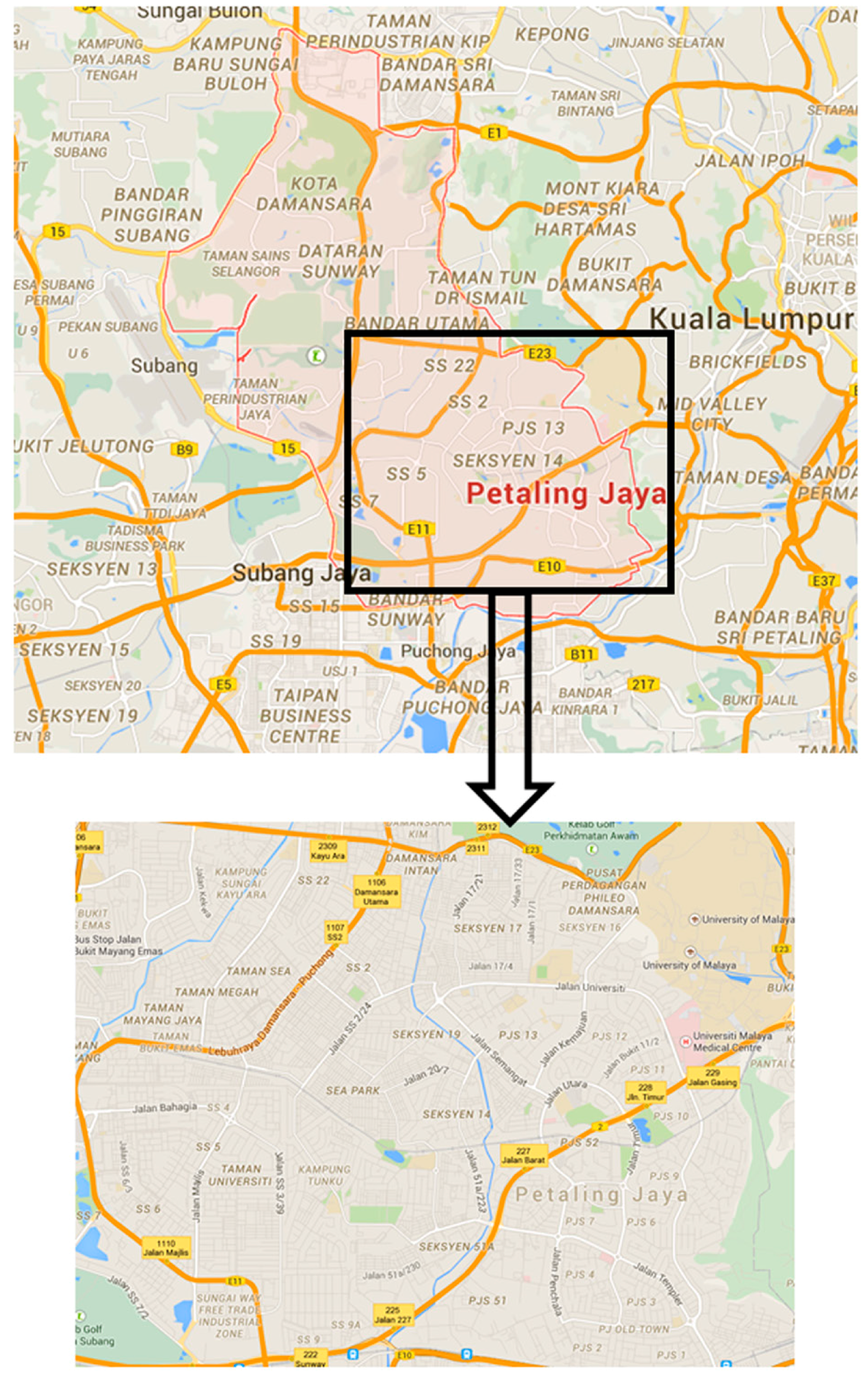
The presented model, explained in detail in Section 3, was applied to the transit services, including bus feeder services connecting the rail stations in the case study (i.e., PJ area). The locations of nodes (i.e., bus stops and rail stations) are given in Table 3 and Table 4. Furthermore, the demand of each bus stop is listed in

Table 6. Passenger demand at bus stops in the Petaling Jaya study area.

Bus Stop No.	Demand (Passenger/h)	Bus Stop No.	Demand (Passenger/h)
1	235	26	20
2	25	27	15
3	35	28	5
4	10	29	5
5	25	30	5
6	85	31	45
7	5	32	40
8	85	33	20
9	15	34	70
10	135	35	10
11	5	36	15
12	25	37	20
13	15	38	55
14	5	39	15
15	70	40	15
16	70	41	10
17	70	42	15
18	40	43	25
19	10	44	15
20	5	45	25
21	20	46	10
22	25	47	15
23	55	48	55
24	30	49	105
25	5	50	20

. The values for the model parameters (e.g., vehicle sizes, operating speed and costs) are specified in

Table 7. Selected values for the parameters used in the Petaling Jaya study area.

Parameter	Unit	Value
μa	RM/passenger-h	28
μw	RM/passenger-h	28
μI	RM/passenger-h	14
λf	RM/veh-h	50.30
λl	RM/veh-km	1.30
λI	RM/veh-h	40
λm	RM/veh-km	2.62
λp	RM/veh-h	35.70
λs	RM/veh-km	0.25
V	km/h	32
Skj	min	15
taF	min	7.5
taTj	min	4
tdT	min/passenger	0.03
tdf	min/passenger	0.096
VT	km/h	40
FT	veh/h	20
fmin	veh/h	2
fmax	veh/h	20
N	veh	100
LF	pass/seat	1
C	pass/veh	36
lmin	km	No constraint
lmax	km	5
λlt	RM /veh-h	630

.

The WCA and ICA techniques have demonstrated their viability as powerful optimization tools with great potential for solving optimization problems [31,32,33,34]. The proposed model and the corresponding optimization methods were coded and run in MATLAB programming software. The optimization procedure for the transit service model involved 50 independent runs, which were performed for each of the considered optimizers.

After performing sensitivity analyses for both optimizers with 50 independent runs, initial parameters for the WCA were a population size of 100, N_sr of eight and d_max of 1 × 10⁻⁵. Accordingly, for the ICA, the initial parameters consisted of a country population of 100, a number of imperialist country of eight and a revolution rate of 0.4.

The application of different optimization algorithms resulted in solutions with diverse precision values. In fact, the solutions state the accuracy of the applied methods and the method’s ability to determine the optimum results. There is a close relationship between the number of function evaluations (NFEs) and the best solutions obtained.

This means that the ideal situation contains the least number of NFEs and is a more accurate solution. With regard to the convergence trend of optimization algorithms and in order to draw a fair comparison between the optimizers, a maximum of 100,000 NFEs was considered the stopping condition for both optimizers.

The number of generated routes is also considered a design variable and varies in a generated population. In fact, the total number of design variables can be changed in this problem in each iteration. Having numerous and changeable design variables can be considered a special feature that can categorize this model as a dynamic optimization model.

The optimization results for the presented optimization algorithms are compared and discussed in this section.

Table 8. Comparison of the best solutions obtained for the transit service model using the reported methods. All cost values are based on Malaysian Ringgit (RM).

Method	CW	Cui	CfF	CmF	CpF	Cu	Co	Cs	CT	AF	TPK
ICA	5042.0	2333.6	688.6	1150.1	1420.3	16,761.3	6815	107.3	23,683.5	5.8	3179.6
WCA	4922.2	2384.7	634.2	1059.2	1497.6	16,692.6	6704	98.8	23,494.8	6.2	3062.4

shows the comparison of the best solutions attained for all cost terms using the applied optimization engines for the improved model. The obtained total cost (C_T) is highlighted in bold in Table 8 for the two reported algorithms.

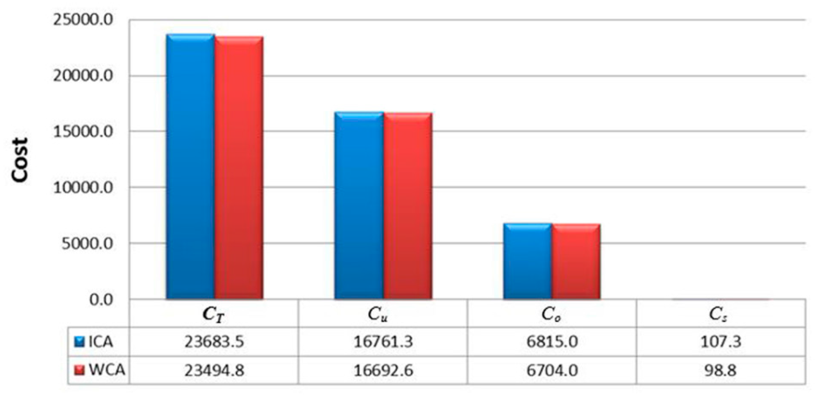
The best solution obtained in the PJ area is provided by the WCA, as shown in Table 8. Additionally, the main costs are illustrated graphically in Figure 4. A total cost of RM 23,494.8 per hour is achieved, with an average service frequency of 6.2 trips per hour (buses on average arriving at intervals of 9.67 min). Accordingly,

Table 9. Comparison of statistical results gained by the optimizers under consideration.

Optimizers	Best Solution	Average Solution	Worst Solution	SD
ICA	23,683.45	24,145.10	24,889.90	242.55
WCA	23,494.80	24,024.00	24,354.05	220.50

demonstrates the comparison of the statistical optimization results obtained for the two reported optimizers for the FNDSP.

Table 9 shows that the WCA obtained the best cost (minimum cost) for the FNDSP. The WCA performed better compared to the ICA, having better solution stability. The detailed statistical optimization results associated with each term in the modified cost function using the applied algorithms are presented in

Table 10. Statistical optimization results for each cost term. All cost values are in RM.

Parameter	Best Solution		Average Solution		Worst Solution		SD 1
	WCA	ICA	WCA	ICA	WCA	ICA	WCA	ICA
CT	23,494.8	23,683.5	24,024.0	24,145.1	24,354.1	24,889.9	220.5	242.6
Cu	16,692.6	16,761.2	16,917.3	17,027.9	17,174.5	17,503.2	123.9	160.7
Co	6703.6	6814.9	6993.4	7002.5	7208.6	7259.4	110.3	91.7
Cw	4922.1	5042.1	5217.8	5232.2	5385.5	5506.6	104.0	95.2
Cui	2168.3	2293.2	2313.9	2409.8	2494.5	2694.7	79.8	103.6
CfF	634.2	680.1	727.7	737.1	792.4	817.3	34.0	28.7
CmF	1059.1	1135.8	1215.6	1231.3	1323.4	1365.4	56.7	48.0
CpF	1412.6	1406.3	1463.0	1439.2	1557.5	1481.9	37.5	17.9
Cs	98.7	106.1	113.4	114.8	123.6	127.4	5.3	4.6
AF	5.1	4.9	5.6	5.4	6.3	5.9	0.3	0.2
TVK	403.49	432.7	463.07	469.1	504.15	520.1	21.65	18.22
TPK	3062.38	3140.62	3350.81	3386.80	3623.83	3867.35	137.96	186.42

¹ “SD” stands for standard deviation, and the values are in RM.

.

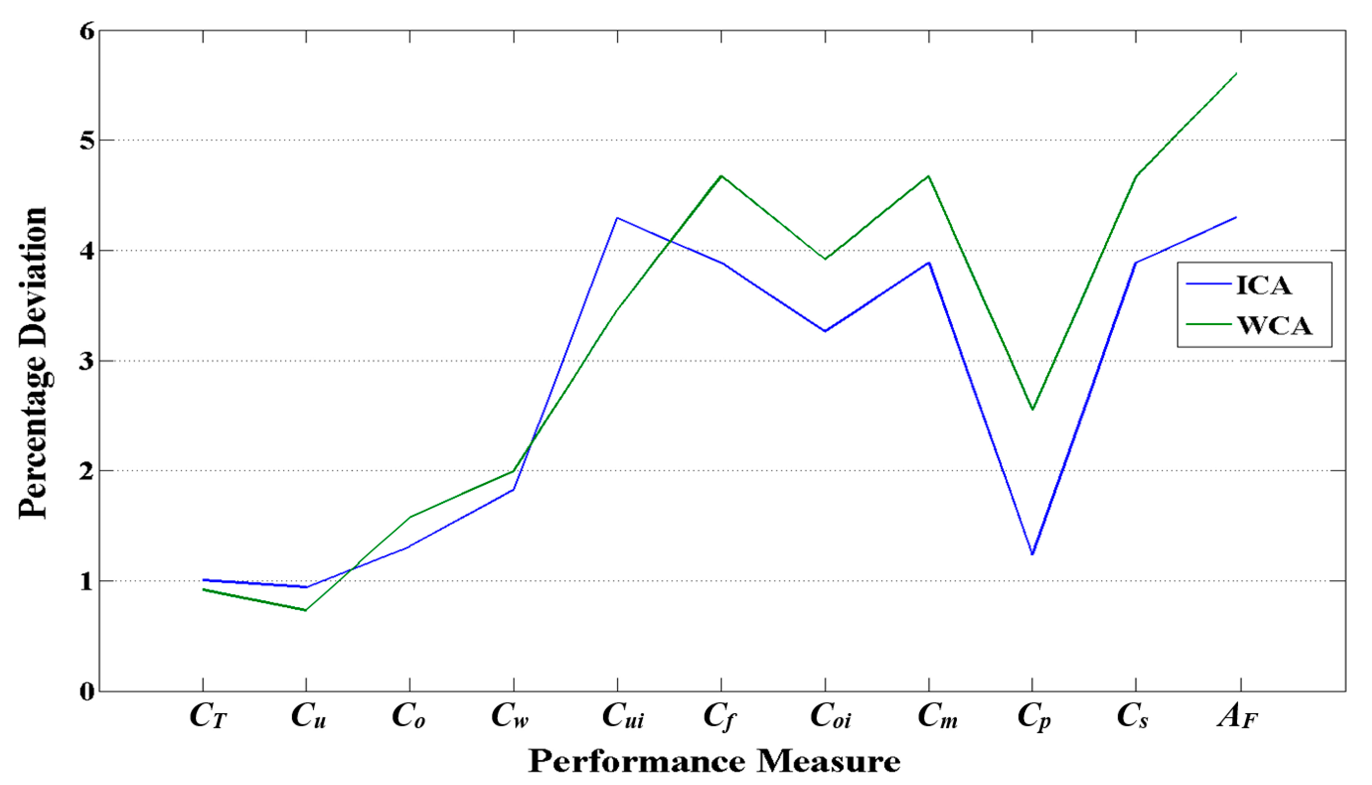
As shown in Table 10, it can be concluded that the WCA is superior over the ICA optimizer for finding all cost terms (except the C_P) with minimum statistical optimization results. Figure 5 shows the deviation percentage associated with the corresponding optimization algorithms for 50 independent runs. Acceptable stability can be seen in the results among different runs.

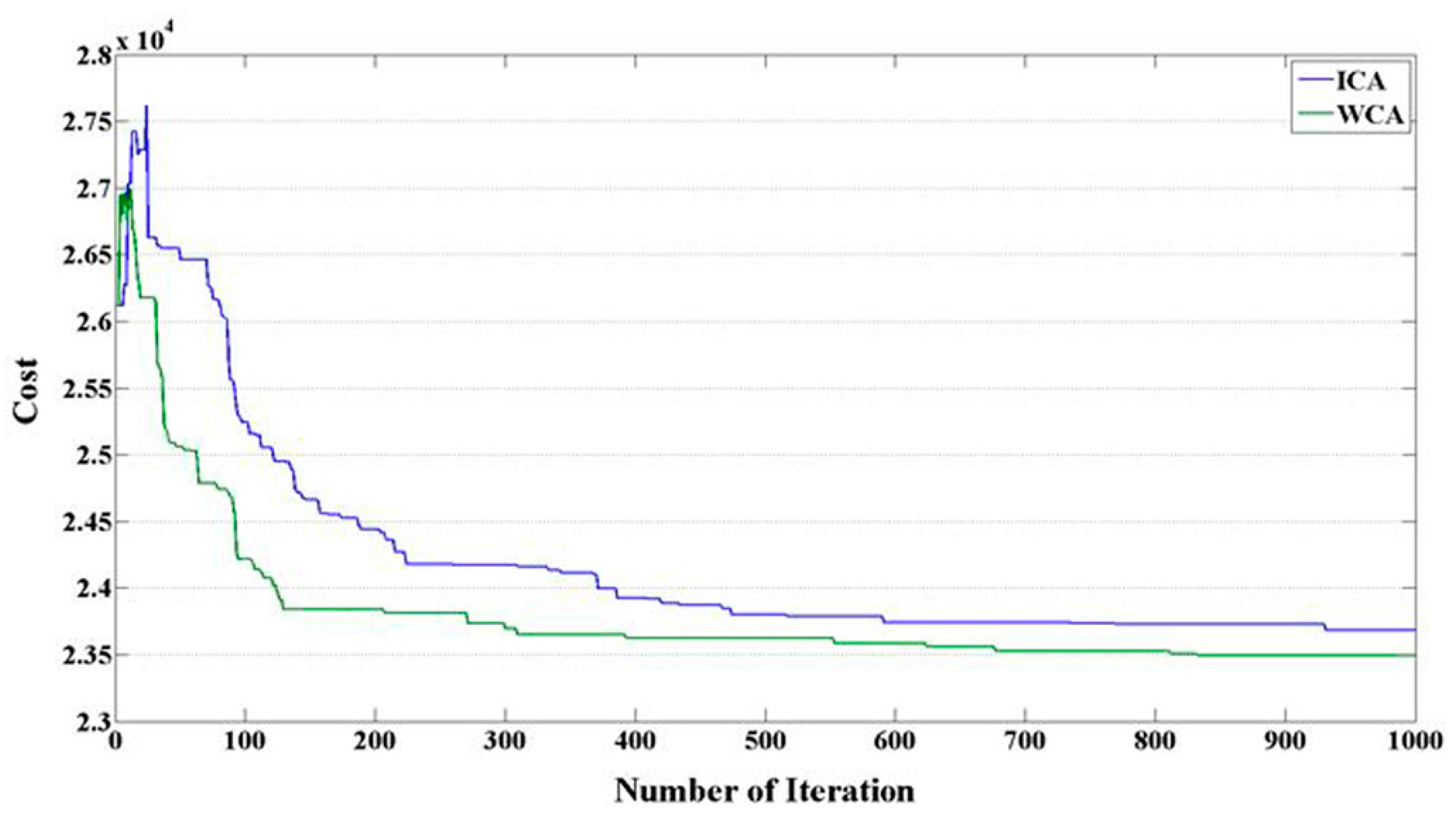
In fact, Figure 5 confirms the reliability of the presented optimization methods. The stochastic nature of the method applied to produce the initial values for each iteration makes it natural not to obtain the same results through different independent runs. However, the final results (C_T) are similar for various runs, with about 0.92% and 1% for the WCA and ICA, respectively. The ICA is only about 0.08% worse than the WCA. Both methods are comparable. The convergence rate and cost history (i.e., cost reduction) of the applied optimization algorithms have been compared and are illustrated in Figure 6.

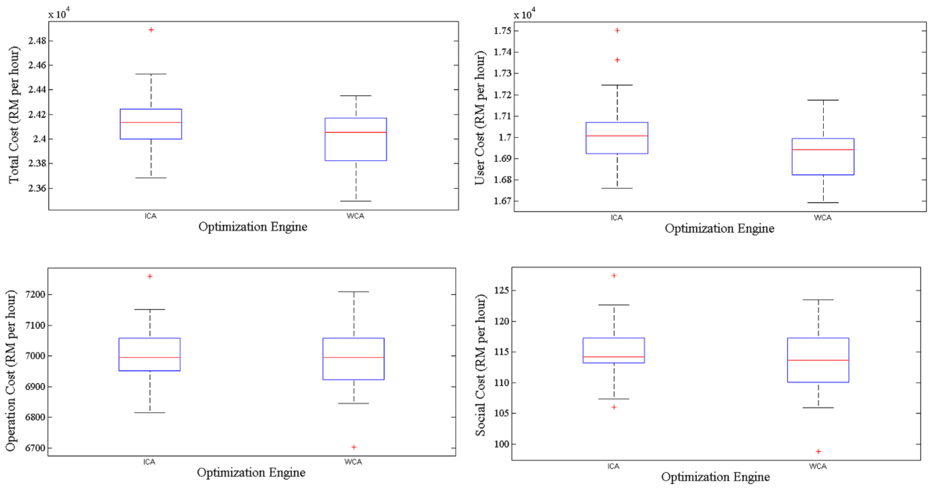
Considering the trend of convergence for each method, the WCA is capable of determining faster optimum solutions with a higher level of precision in comparison with the ICA, as can be seen in Figure 6. It can be observed that the convergence rate for the WCA is faster than the ICA at earlier iterations. Figure 7 illustrates the location and variation of the total cost (C_T) and its main components, namely C_u, C_o and C_s, or 50 independent runs of each optimization algorithm.

It can be observed that the lowest levels for the average cost terms are 24,023.97, 16,917.10, 6993.46 and 113.45, respectively, for C_T, C_u, C_o and C_s with the WCA. The differences between the cost terms of both algorithms for the average cost values are 121, 110.6, 8.9 and 1.5, respectively, for C_T, C_u, C_o and Cs.

It can be highlighted that the lowest level of the average cost in terms of both algorithms becomes nearly the same. However, the ICA shows minimal variation in levels between the first and third quartiles compared to the WCA. In terms of C_T for the ICA, the second and third quartile boxes are approximately the same size. The box plot for that dataset would look like one for a normal distribution, however, with a number of outliers beyond one whisker.

Table 11. Best solution obtained by the WCA. All cost values are in RM.

Route No.	Route Structure		Route Demand (Passenger/h)	Route Length (km)	Route Frequency (Trip/h)
1	51, 1, 2		260	3.50	13.85
2	51, 8, 10		220	1.80	9.59
3	51, 12, 7		30	1.97	3.43
4	51, 13, 11, 5, 4, 3		90	3.01	5.03
5	51, 18, 19, 24		80	2.71	4.95
6	52, 9, 6		100	1.69	6.62
7	52, 16, 17		140	1.14	8.96
8	52, 21, 22, 23, 20		105	3.17	5.31
9	53, 14, 15, 26, 25		100	2.44	5.77
10	53, 29, 28, 27		25	2.00	3.11
11	53, 32, 36, 35		65	2.17	4.87
12	53, 33, 34		90	1.40	6.71
13	54, 31, 30		50	1.33	5.08
14	54, 40, 39, 38, 37		105	2.56	5.80
15	54, 41, 42, 49, 50		150	2.30	7.23
16	54, 43, 45, 48		105	2.15	6.21
17	54, 44, 46, 47		40	2.46	3.63
CT = 23,494.8	Cu = 16,692.6	Co = 6703.4	Cs = 98.8	Cw = 4922.2	Cui = 2384.7
	CfF = 634.2	CmF = 1059.2	CpF = 1497.6	AF = 6.24	TPK = 3062.4

provides the best solution obtained by the WCA among all of the runs, which is illustrated in Figure 8, Figure 9 and Figure 10.

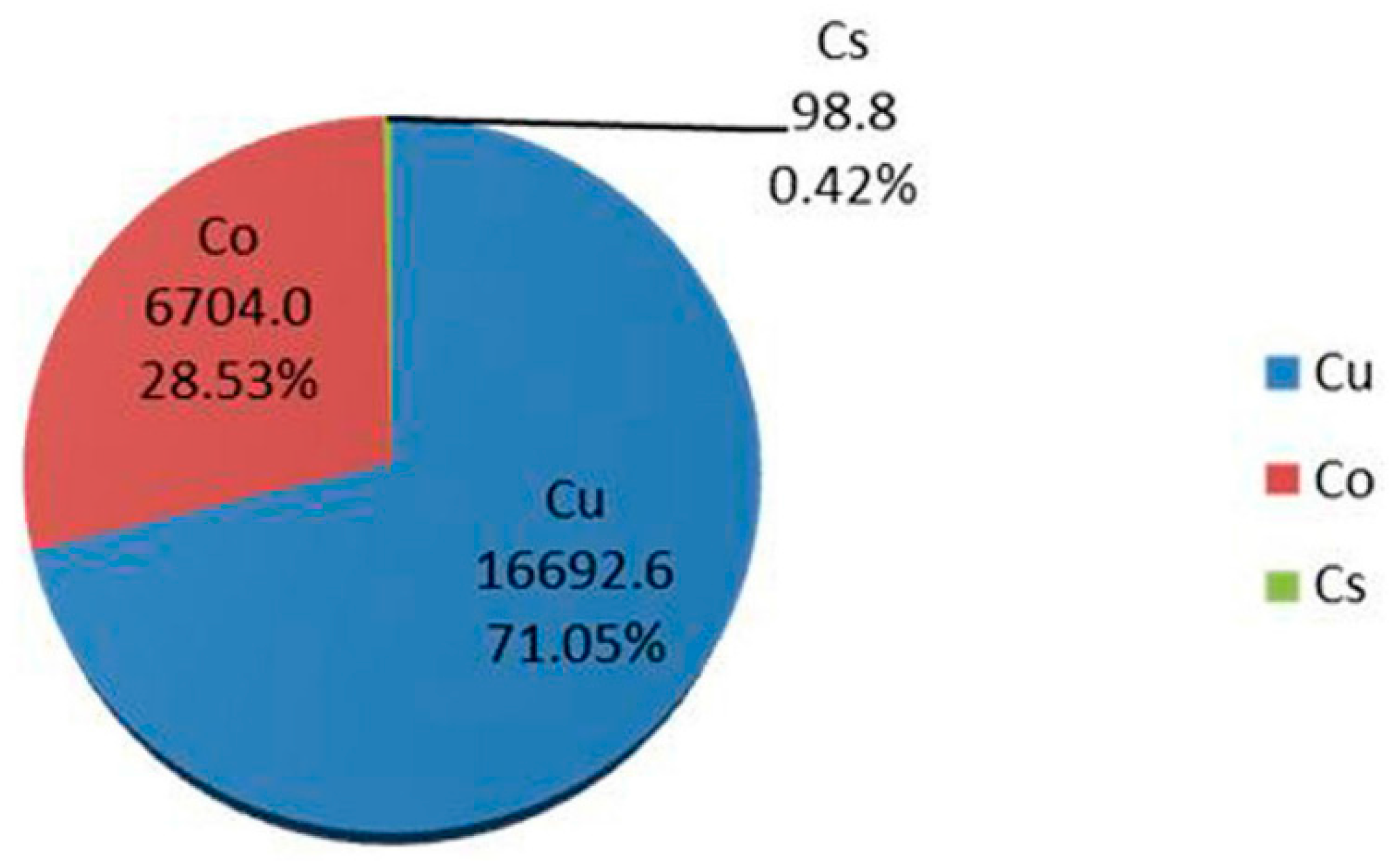
As shown in Table 11, the transit network consists of 17 feeder bus routes with an average service frequency of 6.24 trips per hour (the average headway is 9.61 min). The case solution includes 3062.4 passenger-km of travel. The provided total cost consists of 71.05% user, 28.53% operator and 0.42% social costs, which is illustrated graphically in Figure 8. It can be observed that the main costs are ranked as user, operator and social costs, respectively, from the maximum to minimum.

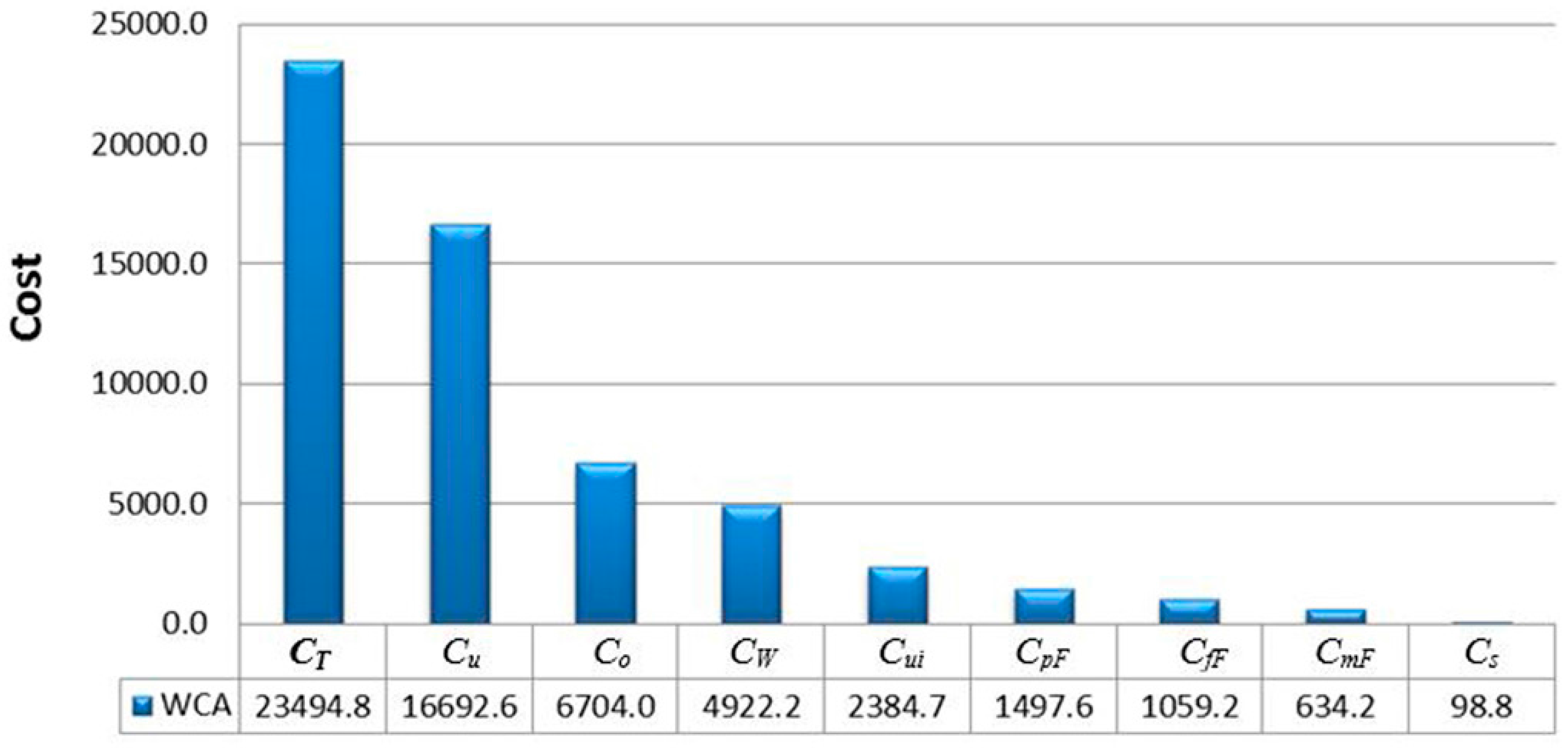
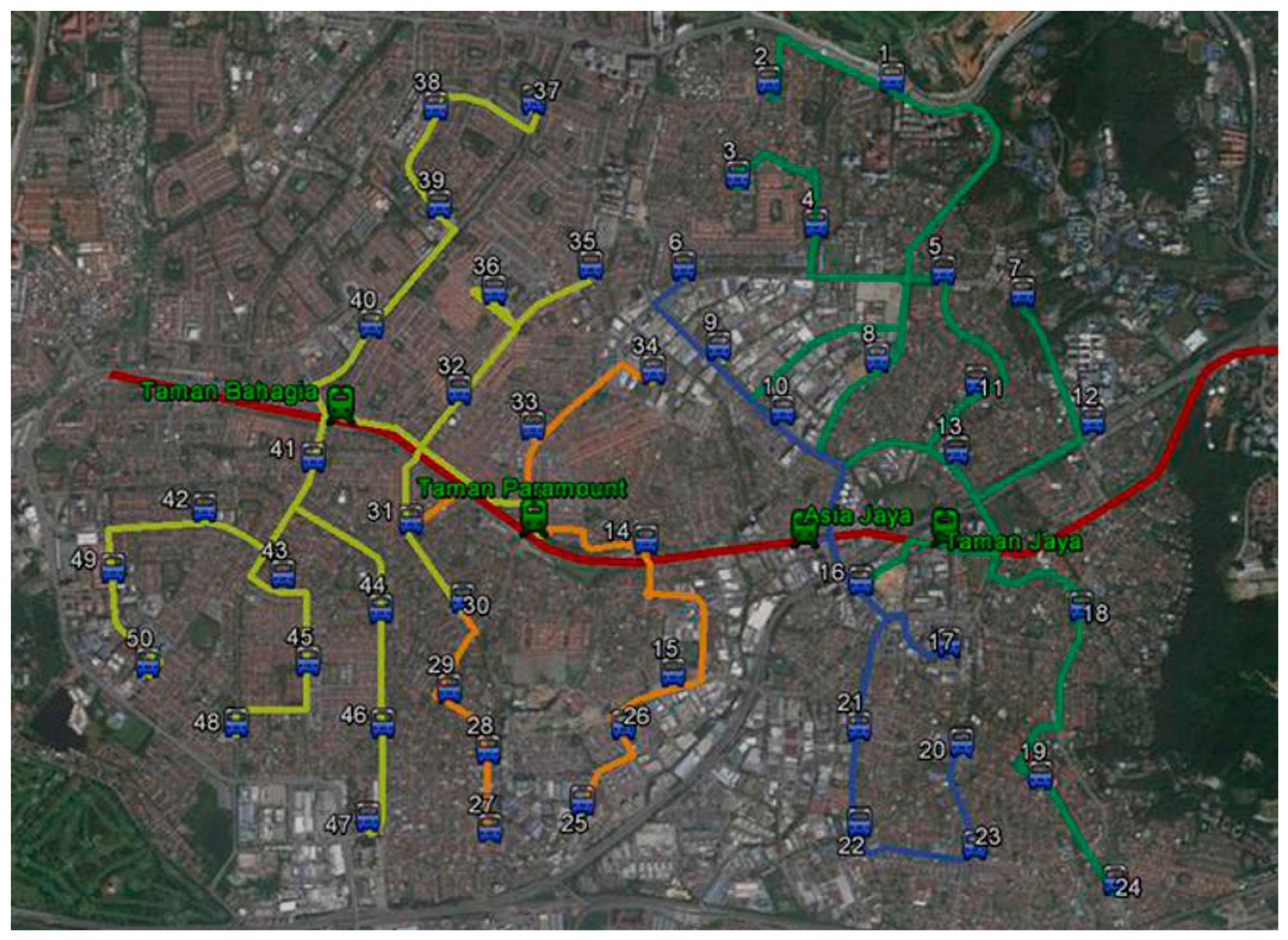
Furthermore, all costs based on RM for each of the cost terms are shown in Figure 9. It is obvious from Figure 9 that the maximum cost of RM 16,692.6 belongs to C_U, while C_s has the minimum cost of RM 98.8. Furthermore, the best transit network obtained by the WCA is given graphically in Figure 10.

The application and optimization of the proposed model to the PJ transit network provided more accurate and efficient solutions for various conditions in the transit systems by employing additional terms and constraints in the objective function. In other words, an effort was made to widen the scope of the research by considering all aspects of satisfaction (i.e., user cost satisfaction, operation cost satisfaction and social cost satisfaction).

Taking into consideration the proposed objective function and imposed constraints, which have already been explained in Section 3, deriving these levels of cost terms shows that the proposed model can be considered a potentially feasible model to overcome current difficulties in the public transit system. This model may lead to the creation of a more realistic model for simulating real-life problems by providing fresh empirical data for future works.

The results of the application and optimization of the transit network design problem in the study area provided more accurate and efficient solutions for various conditions in transit systems. The outputs of these solutions have demonstrated that the presented model has been verified, and the applied optimizers (i.e., WCA and ICA) are considered suitable for obtaining moderate quality solutions under certain computational cost. This confirms the reliability of the presented methodology. Therefore, this model could be considered an alternative model for real transit networks.

7. Conclusions

In this paper, an improved model was suggested for transit network problems, including rail system and feeder bus network designs, as well as frequency setting problems. The main purpose of this paper was to develop a real-life model (actualizing the cost function and adding additional constraints) for handling the feeder bus design and frequency setting problems.

The case study for the research was based on the actual transit network in the Petaling Jaya area, in Kuala Lumpur, Malaysia. Finding the optimum feasible routes in order to reduce the cost function is a vital and difficult task for solving the transit network design problem, which is classified as an NP-hard problem. For this reason, the importance of optimization techniques, particularly metaheuristics, is understood.

Therefore, two recent optimization algorithms, namely the water cycle algorithm (WCA) and the imperialist competitive algorithm (ICA), were considered. The analysis of the objectives shows that the obtained statistical optimization results acquired by the WCA were superior to those attained by the ICA. In terms of solution stability, the WCA also slightly outperformed the ICA.

The optimum number of routes obtained using the WCA was 17, with an average frequency of 6.2 feeder buses per hour in the network. Applying the optimum network resulted in the lowest level of total cost at RM 23,494.8 using the WCA, whereas the corresponding costs obtained by the ICA were about 0.8 percentage points greater than found by the WCA. This confirms the trustworthiness of the presented system. Therefore, the proposed improved model could be considered an alternative model for real transit networks.

Future research may extend the model to consider the stochasticity of the transit and road networks, such as demand uncertainty and variable network performance [3,16,35,36].