Four Sustainability Paradigms for Environmental Management: A Methodological Analysis and an Empirical Study Based on 30 Italian Industries

Abstract

This paper develops an empirical methodology to consistently compare alternative sustainability paradigms (weak sustainability (WS), strong sustainability (SS), a-growth (AG), and de-growth (DG)) and different assessment approaches (LCA, CBA, and MCA) within alternative relationship frameworks (economic general equilibrium (EGE) and ecosystem services (ESS)). The goal is to suggest different environmental interventions (e.g., projects vs. policies) for environmental management at national, regional, or local levels. The top-down methodology is then applied to 30 interdependent industries in Italy for three pollutants and four resources during two periods. The industries were prioritized in terms of interventions to be taken to diminish pollution damage and resource depletion, whereas sustainability paradigms were compared in terms of their likelihood (i.e., WS > AG = DG > SS), robustness (i.e., AG > SS > DG > WS), effectiveness (i.e., SS > AG > DG > WS), and feasibility (i.e., SS > DG > WS > AG). Proper assessment approaches for projects are finally identified for situations when policies are infeasible (e.g., LCA in WS and SS, MCA in DG and SS within ESS, CBA in WS, and AG within EGE), by suggesting MCA in WS within ESS once ecological services are linked to sustainability criteria.

1. Introduction

Environmental problems (from resource exploitation and biodiversity loss to air pollution and climate change) are generating growing concern each day, and have awoken public awareness about trade-offs between economic growth and environmental conservation [1,2]. In this regard, sustainability paradigms can play a crucial role in striking a balance between meeting current and future social needs and protecting the environment from resource overexploitation and pollution production [3].

Among the many alternative definitions of environmental conservation (e.g., maintain eco-system functioning, preserve natural resources, perpetuate eco-system services), the following empirical (i.e., it can be tested from observed data) definition will be used: a situation in which the future status of the environment (F_env) is equal to or better than a certain minimum status (F_env) that is required to preserve its functioning over time (i.e., F_env ≥ F_env). This can be evaluated by referring to both pollution production (i.e., future pollution flows (F_y) or pollution stocks below a given level (F_y), with or without global or local interdependencies) and to resource use (i.e., future renewable or non-renewable use flows (F_x) below a given level (F_x) that implies future renewable or non-renewable resource stocks above a given level, with or without interdependencies in access). In other words, we can achieve environmental conservation if we have low environmental pressure (F_y ≤ F_y and F_x ≤ F_x).

Note that this definition evokes the sustainability concept [4,5] and the ecosystem approach [6,7], together with the precautionary principle [8] and the vulnerability notion [9]. Moreover, the minimum status of the environment could be defined by a political decision that defines the allowed or required flows (e.g., a 40% reduction of greenhouse-effect gas (GHG) emissions below the 1990 level by the EU) or stocks (e.g., the EU authorization to harvest highly migratory species such as tuna, swordfish, and sharks). See the Journal for European Environmental and Planning Law for details on EU directives, decisions, and regulations. Finally, the minimum status could also be defined based on scientific thresholds for flows (e.g., the number of extinct species per million species per year) or stocks (e.g., the concentration of atmospheric CO₂). For an example, see [10].

Among the many alternative definitions of environmental management (e.g., top-down vs. bottom-up, statutory vs. participatory, stable vs. adaptive, centralized vs. collaborative), the following empirical (i.e., it can be tested from observed data) definition will be used: decisions such as policies (e.g., taxes, standards, permits, subsidies, regulations) or projects (e.g., an offshore wave energy platform, a rural forest-based firm) that can achieve environmental conservation. In other words, environmental management can be achieved if environmental decisions lead to decreased pollution production and resource use, thereby generating environmental conservation. Note that current environmental decisions affect the future environmental status both through their effects on stocks and flows of pollution or resources and through whether technical knowledge is incorporated in capital stocks.

Note that this definition neglects, on the environmental side [11], feedback effects [12], non-linearities [13], uncertainties [14], time delays [15], and changes in human behaviors [16] and institutional structures [17] as a consequence of policy interventions. Moreover, current environmental decisions affect the future environmental status both through their effects on stocks and flows of pollution or resources and through whether technical knowledge is incorporated in capital stocks [18,19]. Finally, this definition disregards, on the social side [20], social learning [21] together with information and communication issues [22,23], ethical and educational issues [24,25], social attitudes to uncertainty and ambiguity [26], multiple stakeholder and legal framework issues [27,28], and social participation [29,30] together with collaboration [31,32], coordination [33,34], vertical and horizontal integration [35], adaptation [36,37], and negotiation [38].

However, different environmental interventions (e.g., projects vs. policies), as dependent on alternative sustainability paradigms (e.g., weak sustainability (WS), strong sustainability (SS), a-growth (AG), de-growth (DG)), within alternative relationship frameworks (e.g., economic general equilibrium (EGE), ecosystem services (ESS)), by applying different assessment approaches (e.g., cost effectiveness (CE), threshold analysis (TA), life-cycle assessment (LCA), cost-benefit analysis (CBA), multi-criteria analysis (MCA)), have been suggested to guide the implementation of environmental management.

The purpose of this paper is to develop a methodology for environmental management at the national, regional, or local levels, with the goal of achieving environmental conservation. The top-down, statutory, stable, centralized methodology is applied at the level of individual industries by consistently comparing alternative paradigms, frameworks, and approaches. In particular, sustainability paradigms that are more theoretically likely to lead to environmental conservation are identified, where some policies are suggested in case of unsustainability according to the espoused paradigm, whereas assessment approaches that can be consistently adopted within each sustainability paradigm and relationship framework are discussed in the case of unfeasibility for the suggested policies. Moreover, an empirical application of this methodology to 30 interdependent industries in Italy during two periods (from 1990 to 2007 and from 1990 to 2012), in the context of the abovementioned paradigms operating within the abovementioned frameworks, will show (i) which industry achieves which kind of sustainability; and (ii) which policy can be theoretically and empirically implemented for each industry for three types of pollution (i.e., GHG, rain pollution, air pollution) and four resources (i.e., water, minerals, fossil fuels, biomass). The economically efficient levels of pollution production and resource use are expressed in terms of three crucial features (i.e., environmental concerns, technology, future concerns) in four crucial contexts (i.e., competitive, not competitive, static, dynamic) for two structural parameters (i.e., the natural pollution decay rate, the competitive market interest rate). Pollution production and resource use are normalized to current levels. In other words, my analysis will prioritize industries in terms of the interventions that should be taken to minimize pollution damage and resource depletion, and will compare sustainability paradigms in terms of their likelihood, robustness, effectiveness, and feasibility. Finally, I will discuss assessment approaches that can be consistently adopted within each sustainability paradigm and relationship framework.

Note that a specific kind of response option (i.e., top-down, statutory, stable, and centralized) is focused on. However, each type of response has a distinct set of characteristics, which suggests that they may be best suited to different contexts rather than presumed to be effective in all circumstances. Moreover, many papers evaluate single sustainability indexes based on a small number of indicators in single industries (recent examples: Gadanakis et al. [39] apply a Data Envelopment Analysis to agriculture; Oltean-Dumbrava et al. [40] use a Multi-Criteria Analysis in transport industry; Ali et al. [41] apply a Life Cycle Assessment to agriculture; Branger and Quintori [42] use a Log Mean Divisia Index method in the cement industry). However, there are no studies which measure alternative sustainability indexes based on a large number of indicators in many industries at the national, regional, or local level, and which provide an operational procedure to prioritize interdependent industries in terms of environmental interventions, as well as to identify feasible environmental policies to be implemented at the national, regional, or local level, as dependent on the adopted sustainability paradigm. Finally, a specific kind of response option (i.e., top-down, statutory, stable, and centralized) is referred to. However, a role for those responses can be identified, including regulation, spatial targeting, incentives, and partnership initiatives, in coordination with integrating assessment and planning, without the illusion that they alone can address local or global environmental problems.

2. Methodology

2.1. Paradigms for Environmental Conservation

The purpose of this section is to highlight whether, and under which assumptions, each sustainability paradigm is theoretically capable of achieving environmental conservation. To do so, I developed a series of mathematical formulas that synthesize the factors related to the paradigms and frameworks discussed in the previous section (see Appendix I for the list of abbreviations). I will adopt sustainability for guiding social action rather than considering sustainability as an inherently open principle that provides a framework for discussing the kind of society we wish to have [43].

In the EGE framework, a set of assumptions explains the behavior of supply, demand, and prices in an economy, with many interacting (competitive) markets and with environmental (resource and pollution) relationships. The goal is to seek the set of prices that lead to an overall equilibrium in the quantities of goods [44]. Alternatively, it would be possible to refer to the discounted social utility achieved from consumption of marketed and non-marketed goods, including environmental services and the discounted social utility of traded and non-traded capital stocks, including environmental stocks [45].

The main assumptions behind EGE [46] can be summarized as follows:

• Units of measurement = welfare or utility (U_t, for utility at time t)
• Equity = the same weight is applied to each individual in current and future generations
• Perfect substitution between future and current welfare, i.e., the Kaldor-Hicks criterion

EGE can be formulated as follows:

Arg Max·∫₀^∞ U_t(Z_ecot, Z_soct, Z_envt) e^−σ·tdt

s.t. ∂∂Z_ecot/∂X_t∂t ≤ 0 and ∂∂Z_ecot/∂Y_t∂ ≥ 0

where, Z_ecot, Z_soct, and Z_envt are the current and future economic, social, and environmental features (both stocks and flows and included) at time t, where Z_envt can be split into resources (X_t) and pollution (Y_t) at time t, σ is the social discount rate, and the constraints represent the II and III thermo-dynamic laws (i.e., the increase in entropy and the absence of total recycling, respectively) as a marginal increase in resource use and pollution production for a given level of goods and services. Note that the specification of U_t is uncertain, since future generations could attach a greater value to the environment (i.e., ∂∂U_t/∂Z_envt∂ ≥ 0) [47]. Moreover, inter-generational equity may compete with intra-generational equity unless U_t includes all current generations [48]. Finally, the specification of U_t is uncertain, since future generations could attach a smaller value to consumption (i.e., ∂∂U_t/∂Z_ecot∂t ≤ 0) and rely on more efficient technologies (i.e., ∂∂Z_ecot/∂Z_envt∂t ≤ 0) [49].

Let us assume that the previous dynamic problem with an infinite time horizon can be split into an infinite number of two-period problems, in which t refers to the current (C) period and t + 1 to the future (F) period. In this case, the solution to this problem is a subset of the solutions of the previous problem.

The main assumptions behind WS (i.e., a development that meets the needs of the present generation without compromising the ability of future generations to meet their own needs, where an unconditional substitution among natural, social, and physical capitals is allowed) can be summarized as follows:

• Units of measurement = needs in at least three (i.e., economic, social, and environmental) incommensurable categories
• Equity = possibly different weights for current and future generations
• Perfect substitution between current economic, social, and environmental capitals (Ceco, Csoc, Cenv) as well as between the corresponding future capitals (Feco, Fsoc, Fenv)

WS [50] can be formulated as follows:

Arg Max CU(C_eco, C_soc, C_env) or

Arg Max CU = CW_eco·C_eco + CW_soc·C_soc + CW_env·C_env

s.t. FW_eco·F_eco + FW_soc·F_soc + FW_env·F_env ≥ CW_eco·C_eco + CW_soc·C_soc + CW_env·C_env

and/or F_eco + F_soc + F_env ≥ C_eco + C_soc + C_env and F_eco/F_env < C_eco/C_env

where CW and FW represent the current and future weights of economic, social, and environmental features, with

CW_eco + CW_soc + CW_env = 1, FW_eco + FW_soc + FW_env = 1

CW_eco ≥ 0, CW_soc ≥ 0, CW_env ≥ 0, FW_eco ≥ 0, FW_soc ≥ 0, FW_env ≥ 0

The second objective function is a more specific version of the first one, in which the first and second constraints refer to flows (e.g., welfare) and stocks (e.g., capital), respectively, and the third constraint represents the III thermo-dynamic law. Note that the choice of C_env as the bench-mark is arbitrary. Moreover, the use of many forms of capital combined with the assumption of perfect substitution between types of capital increases the risk for future generations [51]. Finally, the social discount rate is implicitly set at 0 (i.e., σ = 0). Thus, environmental conservation is not pursued, unless C_env = F_env and CW_env = FW_env = 1. The main applications of WS are the following: environmentally adjusted GNP, genuine savings, and an index of sustainable economic welfare. For the relevant concepts, see [52]; for the related measurements, see [53].

A-growth (i.e., an ecological-economic strategy focused on indifference or neutrality about economic (GDP) level and growth as a non-robust and unreliable indicator of social welfare and progress, due to the many neglected non-market transactions (e.g., informal activities and relationships) and the many unpriced environmental effects) [54,55] can be represented as follows:

Arg Min C_env − F_env ≤ 0

s.t. F_soc ≥ C_soc and F_eco + F_soc + F_env ≥ C_eco + C_soc + C_env

Both constraints refer to flows (e.g., welfare) by allowing for substitution between forms of capital. Thus, environmental conservation is pursued, if C_env = F_env, with F_soc ≥ C_soc for social feasibility, and possibly F_eco ≤ C_eco for some sectors.

De-growth (i.e., an ecological-economic perspective based on a socially sustainable and equitable reduction (and eventually stabilization) of materials and energy that a society extracts, processes, transports, distributes, consumes, and returns back to the environment as waste) [56,57] can be represented as follows:

Arg Min F_eco − C_eco ≤ 0

s.t. FW_eco·F_eco + FW_soc·F_soc + FW_env·F_env ≥ CW_eco·C_eco + CW_soc·C_soc + CW_env·C_env

and F_eco + F_soc + F_env ≥ C_eco + C_soc + C_env

where the objective function is measured in production levels, by allowing for the substitution between types of capital. Note that C_eco and F_eco refer to de-growth of production or GDP more than decreased consumption or radical de-growth. Moreover, C_eco could be operationalized as green GDP per capita, which represents per capita GDP after accounting for environmental externalities such as overexploitation of resources and overproduction of pollution. Finally, FW_eco < CW_eco (i.e., decreased future weights attached to economic welfare) could be compensated for by an increase in future weights attached to social or environmental welfare (FW_soc > CW_soc and FW_env > CW_env) to achieve the same CU at smaller C_eco (i.e., decreased consumption or radical de-growth). Thus, apart from its political infeasibility, due to the small importance attached to economic growth (i.e., C_eco > F_eco and CW_eco > FW_eco), and apart from its environmental inefficacy, due to long-run detrimental effects arising from a lack of clean innovation and from a surplus of dirty investments (i.e., (F_env/F_eco) < (C_env/C_eco)), there is no reason to assume that a smaller C_eco will imply a larger F_env: environmental conservation is unlikely to be pursued unless F_soc < C_soc.

The main assumptions behind SS (i.e., a development that allows future generations to access to the same amount of natural resources and the same status of the environment as the current generation, where natural and physical or social capitals are complementary, but not interchangeable) can be summarized as follows:

• Units of measurement = requirements for at least three (i.e., economic, social, and environmental) incommensurable categories
• Equity = possibly different necessities for current and future generations
• No substitution between current forms of capital (C_eco, C_soc, C_env) or between future forms of capital (F_eco, F_soc, F_env)

SS [58] can be formulated as follows:

F_eco ≥ C_eco

F_soc ≥ C_soc

F_env ≥ C_env

In this formulation, alternative environmental indicators (F_env) can be applied, at least at a national or regional level, such as the extent of a forest or the population size of a species, the number of total species, or the (genetic) distribution of a species. Thus, environmental conservation is pursued if C_env = F_env. The main applications of SS are the following: ecological footprints, material-flow accounting, and hybrid indicators. For the relevant concepts, see [52]; for the related measurements, see [53].

In the ESS framework, I will rely on the definition by the Millennium Ecosystem Assessment [59], in which four main ecosystem service functions are identified: provisioning, regulating, cultural, and supporting. Although these choices have been widely criticized for mixing processes (means) and benefits (ends) (e.g., [60]), this classification nonetheless represents an intuitive and useful policy-support tool. For the sake of illustration, these four broad categories will be retained, despite their logical inconsistencies. Alternatively, it would be possible to refer to the ESS definition proposed by The Economics of Ecosystem and Biodiversity project [61]: core ecosystem service processes (production, decomposition, nutrient and water cycling, hydrological and evolutionary processes, ecological interactions), beneficial ecosystem service processes (e.g., R = waste assimilation, water cycling and purification, climate regulation, erosion and flood control, …; S = primary and secondary production, food web dynamics, species and genetic diversification, biogeochemical cycling, …; C = pleasant scenery), beneficial ESS (e.g., P = food, raw materials, energy, physical well-being, …; C = psychological and social well-being, knowledge).

Table 1. Comparison of the economic general equilibrium framework (boldfaced text) vs. the ecological system services framework (normal text) by the Millennium Ecosystem Services Assessment (MEA, 2005). Notes: # includes some insulated and independent supporting services (e.g., biodiversity conservation), if a (simulated) market exists; § includes some insulated and independent cultural services (e.g., pleasant scenery), if a (simulated) market exists.

Provisioning	Renewable #	→	Goods and Services
	Non-Renewable §	→
			↓
Regulating		≠	Pollution
Cultural
Supporting

summarizes the main features of the EGE and ESS frameworks.

The main assumptions behind ESS (e.g., [62]) can be summarized as follows:

• Units of measurement = resistance or resilience for each ecosystem
• Equity = each species or each role of a single species has the same weight
• No substitution between species or between roles of species

ESS can be formulated as follows [63]:

For each ε, η exists such that

|F_env(t₀) − F_env *| < η → for each t ≥ t₁, |F_env(t) − F_env *| < ε

and

∂F_envi(t)/∂t = F_envi(t)·[θ_i − ∑_jⁿ·ζ_ij·F_envj(t)]

where t₀ and t₁ represent the time (t) at the start of the study period and at the return of the systems’ equilibrium, respectively; ε represents the system’s amplitude (i.e., the basin of attraction); η depicts the system’s resistance to small changes, and it is assumed that a circular attractor basin and a deterministic model both exist (see [64] for an alternative basin shape and specification of stochastic models); θ_i depicts the intrinsic growth rate of species i; and ζ_ij represents the impact of species i on species j. In particular, if F_env(t) = (F_env1(t), … F_envi(t), …, F_envI(t)) and F_env * = (F_env1 *, … F_envi *, …, F_envI *) are the vectors for existing species sizes at time t and in equilibrium (*), respectively, there are three consequences: the resistance is measured (i.e., the system’s capacity of small changes in response to external pressures), no substitution between species is allowed, and changes are considered to be detrimental. Alternatively, if F_env(t) = (F_env1(t), … F_envi(t), …, F_envI(t)) and F_env * = (F_env1 *, … F_envi *, …, F_envI *) are the vectors of potential species at time t and in equilibrium (*) to preserve some given relationships between species, respectively, there are three consequences: the resilience is measured (i.e., the system’s ability to retain its functional and structural organizations after perturbations), substitution between species is allowed, and changes are considered to be neither detrimental nor beneficial. Note that the elasticity or recovery is the speed with which the system returns to equilibrium (i.e., the period t–t₀); and the inertia or persistence is the time period in which the system is within ε. For example, if species i could play a role in a desert ecosystem, but it is not present at time t₁, F_envi(t₁) = 0, although this species could replace another species j in this role at time t₂ or subsequently. Similarly, an invasive species could replace more than one current species by preserving the same functional and structural roles within the ecosystem. Of course, the replacement of one species by another implies that both the equilibrium F_env * and the ζ_ij parameters will change.

Table 1 summarizes the main features of the EGE and ESS frameworks.

Note that ecosystem services covers a wider range of consequences than those in an open economic system [65]: ecosystem services do not assume, a priori, that changes to the status quo are either good or bad, whereas open economic systems implicitly consider any change to be bad. Moreover, within the EGE framework, it does not make sense to preserve a non-renewable resource (e.g., oil) indefinitely when its use produces pollution. Finally, ecosystem services cover a narrower range of influences than open economic systems; this is because ecosystem services refer to the indirect benefits obtained from biodiversity through concepts such as resilience, whereas open economic systems stress the direct values obtained from biodiversity through concepts such as existence. In other words, ecosystem services can be used to justify biodiversity conservation for the sake of ecosystem resilience alone, although the modern ability to store genetic resources in a genetics bank may decrease the value of this function. In addition, ecosystem services could justify biodiversity conservation based only on a specified context. For example, biodiversity metrics will differ among spatial scales due to the effects of scale on factors such as the number of species, the genetic distance between species, and relationships among species.

2.2. Policies for Environmental Management

The previous section developed a series of mathematical formulas that, if empirically applied, enable to say which industries are sustainable under each of the paradigms (i.e., WS, AG, DG, SS). In the present section, I will identify policies that are theoretically implementable for environmental management in case of unsustainability by obtaining mathematical formulas for four efficient policies for reducing pollution production (i.e., taxes, subsidies, standards, and permits) and three efficient policies for reducing resource use (i.e., regulations, taxes, and subsidies). These policies are based on three crucial features (i.e., technological improvements, in the form of an increased production level per pollution unit, α ≥ 1; environmental concerns, as a larger perceived damages per pollution unit, γ ≥ 0; and future concerns, in the form of a decreased social discount rate, σ ≥ 0) given two structural parameters (i.e., the natural pollution decay rate, δ ≥ 0, and a competitive market interest rate r ≥ 0). The simplest formulas for optimal levels of pollution production and resource use within the EGE framework are presented in four different contexts (i.e., competitive, non-competitive, static, and dynamic) by assuming that open and closed access for resources can be depicted as competitive and monopoly production markets, respectively, whereas trans-boundary pollution production can be modelled as Nash or cooperative equilibria. The efficient policies are then theoretically compared with environmental management interventions within the ESS framework.

Table 2. Consistency of the four alternative environmental policies with the relationship frameworks and sustainability paradigms.

	EGE	WS	AG	DG	SS	ESS
Policy	Substitute welfare	Substitute types of capital	Substitute types of capital	Complement types of capital	Complement types of capital	Complement species
Permits	C	C *	M	R	I	I
Standards	C	C *	M *	M	M	R
Subsidies	C	C *	M	R	I	I
Taxes	C	C *	M	R	I	I

EGE = economic general equilibrium; WS = weak sustainability; G = a-growth; DG = de-growth; SS = strong sustainability; ESS = ecological system services; C = consistent; I = inconsistent; * = context-dependent; M = potential errors in evaluation metrics; R = potential errors in reference values.

highlights the environmental policies that are consistent with (and suitable for) each paradigm, and therefore indicates to what extent each policy enables managers to achieve the objective specified by each paradigm under the constraints and assumptions made for each paradigm. The prevalence of potential errors in reference values (R) and inconsistent results (I) for taxes, permits, and subsidies in the DG and SS paradigms suggests that it would be necessary to adopt physically based policies for these paradigms, whereas the prevalence of starred C and M for standards in the WS and AG paradigms suggests that it would be necessary to adopt market-based policies for these paradigms. Note that all economically efficient policies are equivalent under the assumptions of the EGE paradigm. Moreover, the ESS paradigm does not account for efficient levels of pollution production and resource use. Finally, perceived damages in the EGE paradigm are mainly based on the evaluations by stakeholders, whereas the ESS paradigm mainly relies on assessments by experts; the appraisals come from an unspecified mix of stakeholder evaluations and expert assessments, but with a lack of information for stakeholders (and in some cases for experts) and a precautionary attitude by experts (and in some cases for stakeholders) in the other paradigms.

In particular, since EGE aims at maximizing the discounted value of social welfare under the assumptions of complete and perfect information as well as competitive markets, economically efficient policies are suitable. In other words, both references and metrics are appropriate. Since WS aims to ensure that future welfare is at least as large as current welfare, economically efficient policies are suitable, provided the assumptions made by EGE hold and provided that the parametrizations required to move from EGE to WS are met. In other words, both references and metrics are contextually appropriate.

Since AG aims at reducing environmental pressure, subject to a non-decreasing social welfare, market-based economically efficient policies are suitable for changing signs (i.e., market demands react to prices), but these might be unsuitable for changing sizes (i.e., perceived damages could be too small to improve environmental status). In other words, references and metrics are suitable and unsuitable, respectively. An efficient standard might be environmentally unsuitable if it imposes too-small fines in terms of the perceived damages, and it might be socially unacceptable if it imposes too-large fines in terms of the perceived damages.

Since DG aims to reduce production levels in dirty industries, subject to a non-decreasing total capital, market-based economically efficient policies are unsuitable for changing signs (i.e., perceived damages could be biased in identifying dirty industries), but might be suitable for changing sizes (i.e., market demands react to prices). In other words, references and metrics are unsuitable and suitable, respectively. A standard is environmentally suitable, provided the fines are large enough, but it could be socially unacceptable.

Since SS aims at making the future environmental status at least as good as the current one, market-based economically efficient policies are unsuitable when market demands are missing (and consequently there are no price values) or when damage perceptions are biased or absent (due to lack of knowledge or information). In other words, both references and metrics are inappropriate. A standard is environmentally suitable, provided the fines are large enough, but it could be socially unacceptable if the fines are too high. Since ESS aims to preserve ecological resilience, market-based economically efficient policies are unsuitable whenever market demands are missing and damage perceptions are biased or absent. In other words, both references and metrics are inappropriate. A standard is unsuitable whenever direct or indirect uses are absent.

Note that I here refer to suitability of policies in terms of goals specified by each paradigm rather than in terms of environmental conservation: in Section 4.2, effectiveness will highlight if a paradigm properly tackles environmental issues by identifying which tool is consistent with which paradigm, and feasibility will highlight if these tools are feasible in terms of environmental conservation. Moreover, since a smaller spatial scale is likely to reduce the significance of incomplete or asymmetric information and of market competition, standards might be more appropriate at a local level. Similarly, the policies suitable for the ESS framework could require the introduction of some species or a change in physical conditions at a local level to improve the resilience of the local ecosystems. Finally, the optimal single policies in terms of EGE efficiency are obtained, although a shift from policies on resource use to policies on pollution production might be required if the use of a resource generates pollution (e.g., combustion of fossil fuels). Similarly, a shift from the EGE framework to an ESS framework might be required if the efficient use of a resource damages one or more ecological services (e.g., stream water).

Pollution production within the EGE framework can be represented as follows:

Max ∫₀^T·p·Q − FC − ½·β_Q·Q² − ½·β_E·(E–E₀)² − ½·(γ/α)·Q² + sub (Q₀ − Q) e^−σ·t·dt

s.t. ∂Y/∂t = Q + q − δ·Y with interaction, ∂Y/∂t = Q − δ·Y with no interaction

where

E = Q/α and β_Q + β_E = 1

where p is the price of a production unit; Q and Q₀ are the production levels at time t and 0, respectively; FC represents fixed costs, β_Q is the production cost per production unit, β_E is the abatement cost per pollution unit, E and E₀ are the effluent level at time t and 0, respectively; γ is the perceived damages per pollution unit, α is the production level per pollution unit, σ is the social discount rate, q is the level of production at time t outside the spatial scale under consideration (i.e., other countries, other industries), δ is the natural pollution decay rate, and sub is the magnitude of the subsidy when production levels are smaller than Q₀. Note that producer surpluses represent profits if FC = 0, and β_E = 0 (i.e., β_Q = 1) if reducing production is the only way to reduce pollution.

Table 3. Optimal flows and stocks of pollution production within the EGE framework (from Zagonari, 1998 [66], where α = A become p, β becomes γ/α, B becomes Γ/A).

	Static (Flows Are Relevant)		Dynamic (Stocks Are Relevant)
In	Nash YNashS = 2p/[1 + (Γ/A) + (γ/α)]	Coop YCoopS = 2p/[1 + (2Γ/A) + (2γ/α)]	Nash (if Σ = σ = Γ = 0) YNashD = 2p·δ/[(γ/α) + δ2] if δ2>γ/α with M = 0 and μ = −2(p·γ/α)/[(γ/α) + δ2]	Coop (if Σ = σ = 0) YCoopD = 2p·δ/{2[(γ/α) + (Γ/A)] + δ2} with μ = −2p([(γ/α) + (Γ/A)]/{2[(γ/α) + (Γ/A) + δ2]}
No	YNoS = p/[1 + (γ/α)] + p/[1 + (Γ/A)]		YNoD = p·δ/[(γ/α)+δ2] + p·δ/[(Γ/A)+δ2] if Σ = σ = 0 with M = −[p(Γ/A)]/[(Γ/A) + δ2] and μ = −[p(γ/α)]/[(γ/α) + δ2]

In = interaction; No = no interaction; Nash = Nash equilibrium conditions; Coop = cooperative conditions; S = static conditions; D = dynamic conditions; Y_NashS > Y_CoopS, Y_NoS > Y_CoopS, Y_NoS > Y_NashS if γ/α > Γ/A−1.

identifies the optimal flows and stocks of pollution production within the EGE framework in the cases with and without interactions.

Note that only linear strategies are considered in the present study: see [66] for a discussion of non-linear strategies. Next, if the social discount rate σ is assumed to be 0, optimal pollution production in a dynamic context equals that in a static context, whenever δ = 1.

Thus, the suggested policies in the static context for a single polluter without interactions are the following, where the socially optimal level of production Q* = p/[1 + (γ/α)] maximizes total net benefits (i.e., Max p·Q − FC − ½·β_Q·Q² − ½·γ/α·Q² if and only if the first-order condition is met p − Q − (γ/α)·Q = 0 and the second-order condition is met −1 − (γ/α)<0):

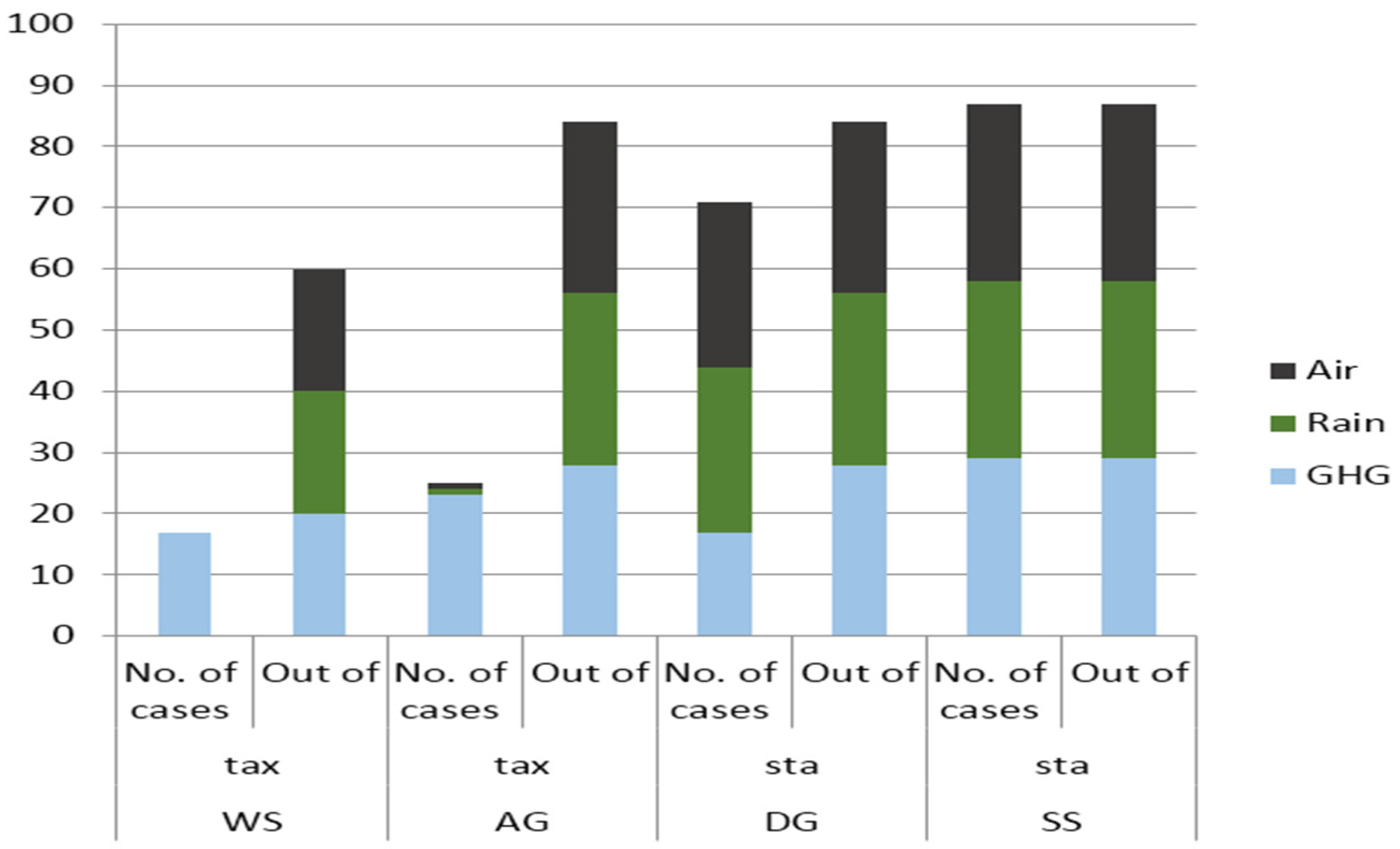
• A tax * = γ/(γ + α), which arises from p·(1 − tax) − Q* = 0 (i.e., the net marginal benefit is 0)
• A subsidy sub* = {−α + √[(2α + γ) (4α + γ)}/(2α + γ) with Q₀ = FC = 1 (i.e., sub is decreasing in α and increasing in γ, whenever γ is large enough), under the assumption of a linear and normalized demand (i.e., Q = 1 − p), by dividing by the maximum production level, and Arg min AvC = √(2(FC − sub Q₀)) ≤ √(2FC) (i.e., each firm produces less), p = min AvC = sub + √(2(FC − sub Q₀)) ≥ √(2FC) (i.e., the long-run equilibrium price with a subsidy must be larger than that without a subsidy) if and only if 0 ≤ sub ≤ 2(√(2FC) − Q₀), and Q = 1 − p = 1 − min AvC = Q* = p/(1 + (γ/α)) = min AvC/(1+ (γ/α)), where AvC is the average production cost)
• A standard sta* at Q *, coupled with the optimal fine (γ·p)/(γ + α) = p·tax*
• Permits issued in quantity E* = Q*/α and traded at price per* = (∏β_E/∑β_E)(∑E₀ − E*), which arises from marginal cost MgC = p = β_E·(E₀ − E) (i.e., the marginal abatement cost equals the permit price), E = E₀ – (per/β_E) (i.e., the demand for permits by each firm), E* = ∑E = ∑(E₀ – per*/β_E)

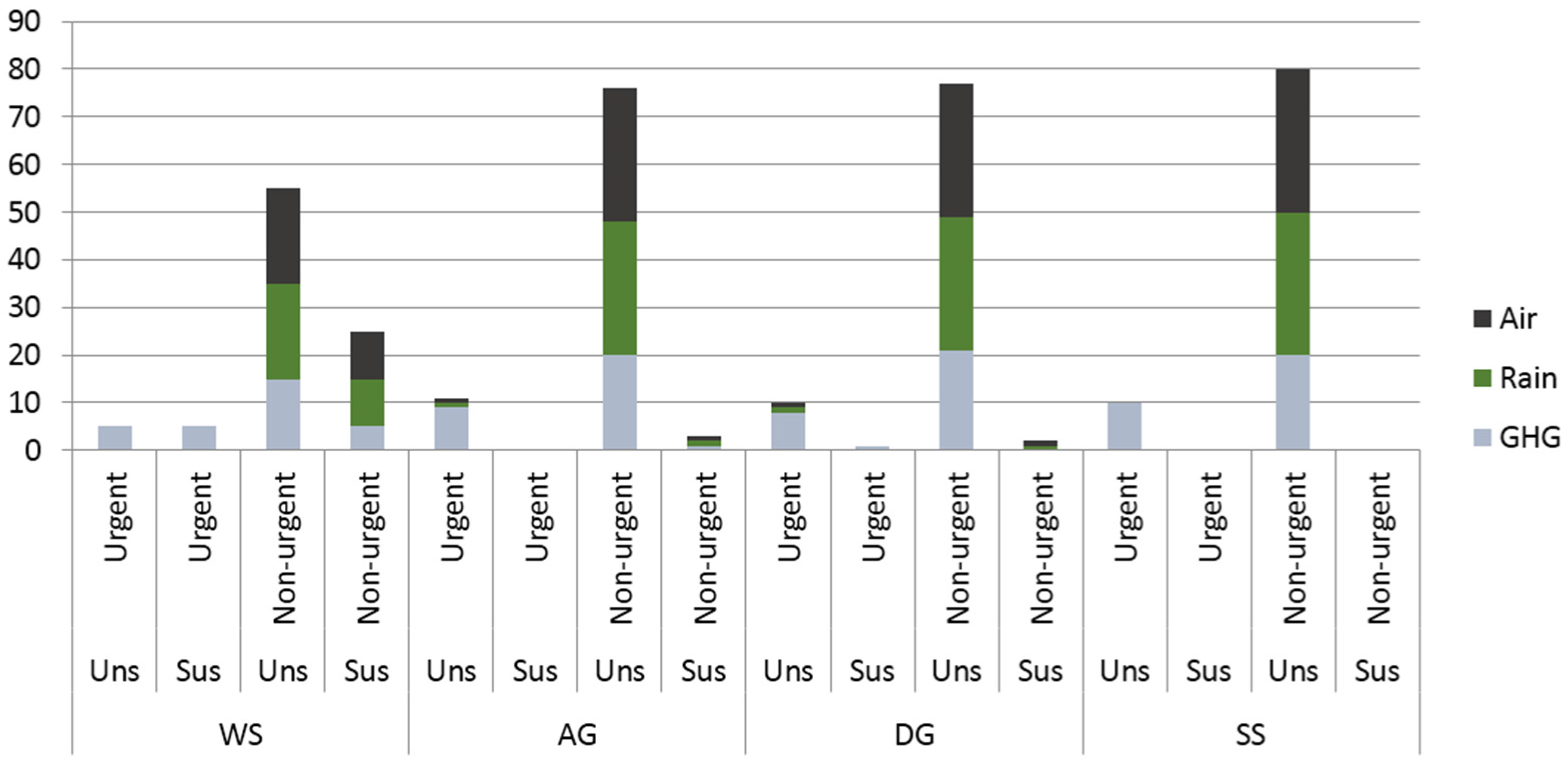
Similar results are obtained for the other three contexts (i.e., static with interaction, dynamic without interaction, dynamic with interaction). However, environmental conservation might not be achieved whenever γ is too small, since it represents perceived external effects (preferences) by current generations, or α is too small, since it represents external effects (technologies) produced by current generations (i.e., Q*/α = E* > Y).

Renewable resource use within the EGE framework can be represented as follows:

Max ∫₀^T·p·H – [(w·H²)/X]·e^−r·t·dt

s.t. ∂X/∂t = f(X) − H = a·X − b·X² − H

where T is the final time, p is the resource price, H is the harvest rate at time t, w is the wage rate, X is the resource stock, r is the competitive market interest rate (which is usually larger than the social discount rate σ), f(X) represents the natural growth (which is a function of the resource stock), a and b depict a quadratic formulation of the function f(X), and FC = 0 if H is normalized to 1, by dividing by the maximum harvest level. Note that the model presented above can be achieved by fixing Q = H whenever a resource use produces pollution (e.g., soil erosion from forest cutting). Next, w could include both perceived overexploitation costs, as depicted above by γ, and technological improvements, as depicted above by α (e.g., w = (w′ + γ)/α, with w′ representing the labor wage rate without these additional features). Here, α = 1 and γ = 0.

Table 4. Optimal flows and stocks of renewable resources within the EGE framework.

	Static (Flows Are Relevant)	Dynamic (Stocks Are Relevant)
In	XInS = w/p ≤ a/b	If p = (wH)/X (μ = 0), XInD = a/b − (1/b)(p/w) (medium); XInD = a/b (long)
No	XNoS = ½ [(a/b)+(w/p)] ≤ a/b	XNoD = (a − r)/(2b) − p/(b·w) + {√(4·p2 + (a·w + r·w)2)}/(2b·w) (medium and long) with μ = {√(4·p2 + (a·w + r·w)2)}/2 − [(a·w + r·w)/2]; If w = 0 (μ = p), XNoD = ½ (a − r)/b (medium and long)

In = interaction; No = no interaction; S = static conditions, D = dynamic conditions; X_NoS ≤ a/b if p ≥ w (b/a); X_NoS > X_InS since X_InS ≤ a/b, X_InD < X_InS, X_NoD < X_NoS; medium = long-run stable conditions for X only; long = long-run stable conditions for both X and μ.

identifies the optimal flows and stocks of renewable resources within the EGE framework.

Note that the equilibrium stock in the dynamic model with interaction becomes the equilibrium stock in the static model with interaction if p = 0 (i.e., no economic returns from resource use). Similarly, the equilibrium stock in the dynamic model with no interaction becomes the equilibrium stock in the static model with no interaction if r = 0 (i.e., no discount factors for future economic returns).

Thus, the suggested policies in the static context (e.g., fresh water) are the following:

• In DCs (i.e., a/b ≤ w/p), support market competition by favoring the use of licenses, and increase w (e.g., license prices), decrease p (e.g., implement a value-added tax [VAT]), or do both.
• In LDCs (i.e., a/b ≥ w/p), interfere with market competition by blocking use of licenses, and increase a (e.g., network efficiency), decrease b (e.g., network leakages), or do both.

Thus, the suggested policies in the dynamic context (e.g., harvest forests, catch fish) are the following:

• In the case of strong competition in the market, the industry will disappear: no intervention is required.
• In the case of weak competition in the market, in LDCs with a small real production cost (a small w), reduce the number and use of licenses, by increasing a (e.g., smaller proportion of harvested forest, larger fish net sizes), decreasing b (e.g., protected land, protected sea) at a given (large) return from capital markets (r). In DCs with a large real production cost (a large w), increasing w (e.g., taxes on input fuels), decreasing p (e.g., implementing a VAT), or both could also be effective, at a given (small) return from capital markets (r).

However, there might not be a set of a, b, w, and p at a given r such that X ≥ X = 0 (i.e., no extinction of resources), due to social sustainability considerations.

If the resource price depends on its stock p(X) and if H = 1, so that the focus is on the final time (T) and initial price (p₀) rather than the harvest rate (H), and if C(X) = 0 so that p becomes the marginal surplus, then the previous maximization problem for renewable resource use boils down to the following dynamic equations for non-renewable resource use within the EGE framework:

XT = X₀ − ∫₀^T·p_k − p₀·e^r·t·dt

p_T = p₀·e^r·T

where X₀ is the initial stock, p_k is the largest demand for a non-renewable resource, and r is the competitive market interest rate, which is usually larger than the social discount rate (σ). Note that technological improvements, as depicted above by α, imply an increase in p₀, the initial marginal surplus (i.e., p₀ = p₀’ × α, where p₀’ is the initial price without technological improvements); here, α = 1. Moreover, p_T could include the perceived external costs from pollution due to the use of a non-renewable resources, as depicted above by γ (i.e., p_T = p_T’ − γ, where p_T’ is the final price without external costs); here, γ = 0. Finally, technological improvements, as depicted above by α, imply an increase in the feasible stock of non-renewable resources (i.e., X₀ = X₀’ × α, where X₀’ is the initial stock without technological improvements); here, α = 1.

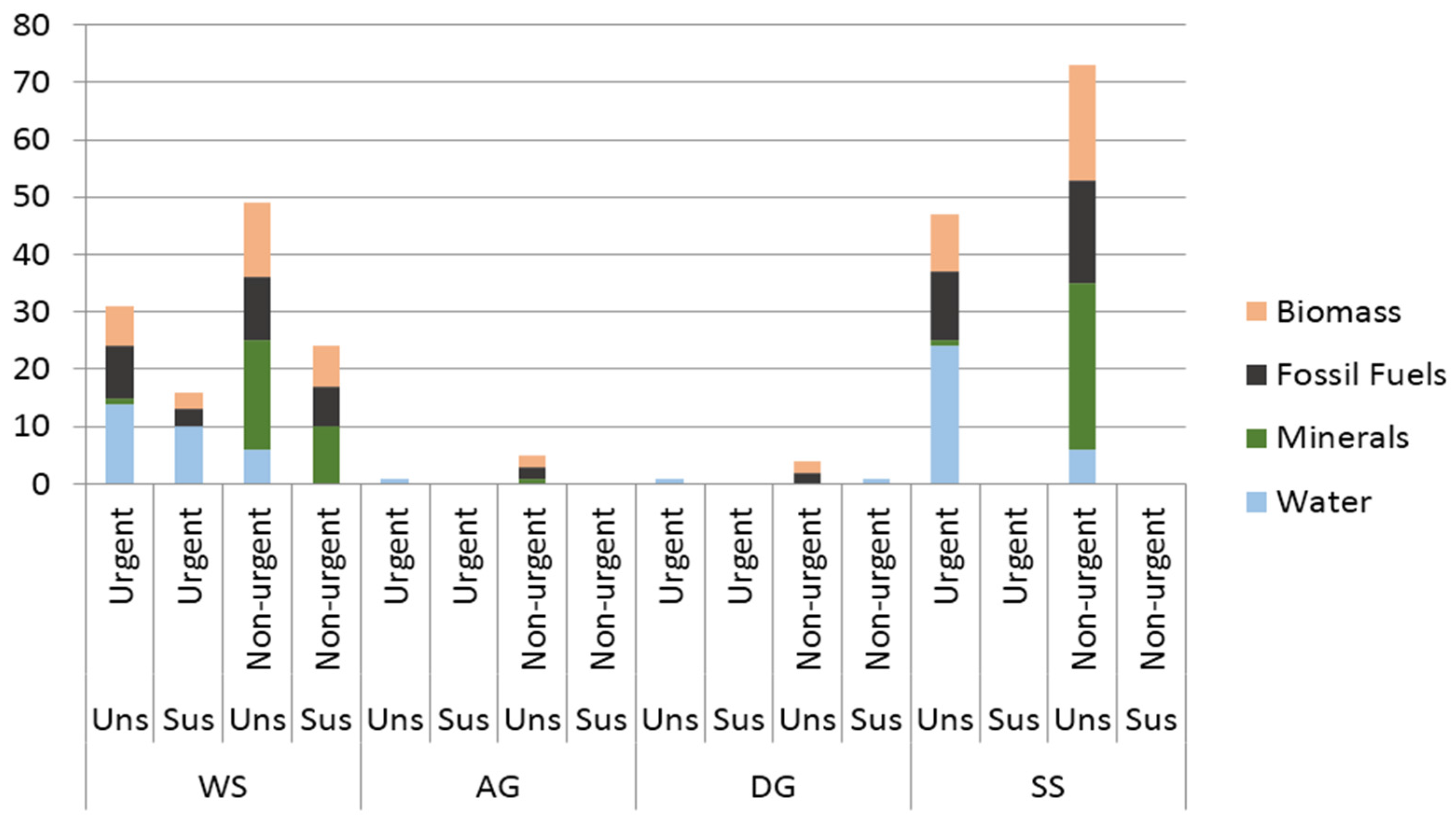
Instead of solving these equations with respect to T and p₀ in terms of X_T for a given X₀ and p_k, these equations are solved with respect to X_T by setting p_T = p_b, defined as the price of an alternative less-polluting resource b, by eliminating T, and by setting X_T = X_b, which is defined as the stock of a non-renewable resource that is left unused when it is replaced by an alternative less-polluting resource b; whenever a resource use produces air pollution (e.g., minerals) or GHG pollution (e.g., oil), a larger X_b means smaller resource flows for any given X₀.

Table 5. Optimal stocks of non-renewable resources within the EGE framework. In = interactions; No = no interactions.

	Dynamic (Stocks Are Relevant)
In	If pk = p0 so pb = p0, XIn = X0 − (p0/r) with XIn → X0 if p0 → 0
No	If pk > p0 and pb > p0 with pk > pb, XNo = X0 + ((pb − p0)/r) − (pk/r)·ln(pb/p0)

identifies the optimal stocks of non-renewable resources within the EGE framework.

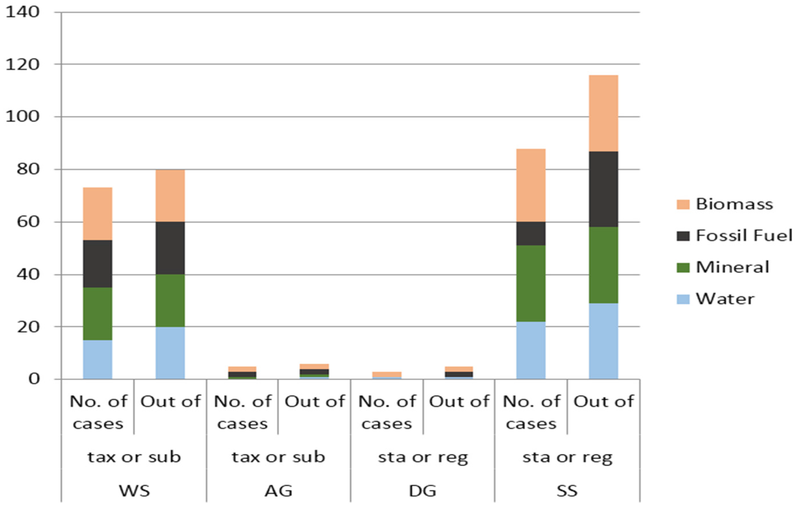
Thus, the suggested policies for non-renewable resources with impacts on air pollution (e.g., minerals in competitive markets) or GHG pollution (e.g., oil in non-competitive markets) are the following:

• In the case of strong competition in the market, decrease p₀ (i.e., ∂X_In/∂p₀ = −(1/r) < 0; e.g., indirect taxes on minerals), at a given r.
• In the case of weak competition in the market, at given r, increase p₀ (i.e., ∂X_No/∂p₀ = (1/r) ((p_k/p₀) − 1) > 0; e.g., indirect subsidies on oil), decrease p_k (i.e., ∂X_No/∂p_k = −(1/r)·ln(p_b/p₀) < 0; e.g., create an information campaign to replace oil with alternative fuels), and decrease p_b (i.e., ∂X_No/∂p_b = (p_b − p_k)(r p_b) < 0; e.g., subsidize substitutes for oil).

However, there might not be a set of p₀, p_b, p_k, and r such that X ≥ X (i.e., low levels of air and GHG pollution), due to social sustainability constraints.

2.3. Projects for Environmental Management

The previous section highlighted four efficient policies for reducing pollution production (i.e., taxes, subsidies, standards, and permits) and three efficient policies for reducing resource use (i.e., regulations, taxes, and subsidies) that are theoretically implementable for a given unsustainable industry. The purpose of this section is to identify which project assessment approach would be appropriate in each relationship framework and sustainability paradigm, if policies are empirically infeasible. In this context, plans can be considered to represent complex combinations of policies and projects.

Note that market-based policies are theoretically infeasible if there are no markets or if it is impossible to simulate markets (e.g., for some cultural or supporting services), whereas projects can always be implemented. Moreover, I will disregard situations where combinations of projects rather than a single project, characterized by different features (e.g., access rights or regulating services) in different contexts (e.g., incomplete or asymmetric information), must be compared with the no-project option. Finally, policies should be preferred to projects if the environmental conservation issues are similar for many industries and if a similar environmental management policy can be implemented.

Since cost effectiveness and threshold analysis can be depicted as special cases of CBA, I will only explicitly compare CBA (i.e., a systematic set of rules for comparing economic benefits and costs (expressed in monetary terms) of alternative potential interventions (projects, decisions, policies) to maximize social welfare), MCA (i.e., a systematic set of methodologies for structuring decision problems involving more than one criterion to find non-dominated alternative solutions, by incorporating preference information), and LCA (i.e., a systematic set of phases for comparing the full range of environmental effects (expressed in terms of water, energy, materials) associated with all stages of a product’s life to support business strategies and to improve product and process designs), if single issues are relevant, by disregarding combined issues (e.g., time and economic interdependencies, to be analyzed by game theory within CBA; time and uncertainty, to be tackled by stochastic dynamic programming within CBA or real options analysis potentially within CBA, MCA or LCA; and uncertainty and economic interdependencies, to be analyzed by game theory within CBA).

If time and space are relevant, the net present value is common to CBA and MCA, whereas the benefit–cost ratio and internal rate of return are peculiar to CBA, where the benefits and costs are assumed to be properly evaluated. Time is crucial in any LCA, whereas space is considered in versions of LCA that are based on donor-side (i.e., production) sources for energies (e.g., emergy in [67,68]), user-side (i.e., consumption) destinations for energies (e.g., exergy in [69,70]), and recycled content (i.e., production) for materials (e.g., [71,72]); in contrast, space is disregarded in versions of LCA based on end-of-life recycling (i.e., consumption) for materials (e.g., [73,74]).

In the case of uncertainty, the sensitivity analysis, Monte Carlo simulations, fuzzy analysis, the technique for order of preference by similarity to ideal solution (TOPSIS), and the expected-value approach are common to both CBA and MCA, whereas the expected-utility or mean-variance approaches are peculiar to CBA, with probabilities determined under the assumption that benefits and costs are properly evaluated. If the best outcome is 1 and the worst outcome is 0, and if losses = −gains, then linear TOPSIS is equivalent to the expected utility approach with risk neutrality. Under the assumption of a normal distribution or a quadratic utility function, expected-utility and mean-variance approaches are equivalent. A risk-averse approach [75] prevails in versions of LCA based on recycled content for materials (e.g., [76]), but risk-tolerant or risk-seeking approaches [75] prevail in versions of LCA based on end-of-life recycling for materials (e.g., [77]).

If inter-generation and intra-generation equity are relevant, CBA uses a social welfare function, whereas MCA introduces weights, although the max-min function (i.e., the goal is to maximize the minimum benefit) is common to CBA and MCA. Versions of LCA based on user-side destinations for energies and recycled content for materials (e.g., [78]) stress intra-generation equity, as does the integrated environmental and economic form of LCA (e.g., [79]), whereas versions of LCA based on donor-side sources for energies (e.g., [80]) and end-of-life recycling for materials focus on inter-generation equity.

Table 6. Suitability of CBA, MCA, and LCA for dealing with various issues.

	CBA	MCA	LCA
Time	S (dynamic programming)	S	S
Space	S	S	RC, Em, Ex
Uncertainty	S (stochastic programming)	S	RC, EoLR
Intra-generation equity	S (social welfare function)	S (weights)	RC, Ex
Inter-generation equity	S (social welfare function)	S (weights)	EoLR Em
Economic interdependencies (e.g., markets)	S (if modelled)	U	IEE
Social interdependencies (e.g., rights)	S (if modelled)	U	U
Ecological interdependencies in time and space	U	S	Em

S = suitable; U = unsuitable; EoLR = end-of-life recycling; RC = recycled content; Em = emergy-based LCA (donor-side); Ex = exergy-based LCA (user-side); IEE = integrated environmental and economic versions of LCA.

summarizes the suitability of CBA, MCA, and LCA for tackling these various issues.

In the case of ecological interdependencies, MCA should be preferred to CBA. Indeed, CBA assumes a perfect competitive set of markets with resources as inputs and pollution as outputs, where the marginal evaluation is external to the ecological processes and services, and it arises from prices being equal to marginal opportunity costs. Thus, CBA is consistent with an impact-based approach. In contrast, MCA can account for ecological interactions and equilibria, with some processes and services being beneficial to humans, and the assessment in percentages is internal to the ecological processes and services. Because it has nothing to do with prices, it is consistent with a change-based approach. Some donor-side versions of LCA (e.g., emergy in Sustainability Index by [81]) do not apply an impact approach.

If economic and social interdependencies are relevant, CBA should be preferred to MCA. Indeed, CBA assumes a perfectly competitive set of markets with complete or incomplete rights or contracts, and with the marginal evaluation internal to the economic and social interactions (e.g., Nash equilibria). This arises from prices being equal to marginal opportunity costs, with potential distortions (e.g., monopolistic power). In contrast, MCA can refer to the social and economic interactions and equilibria, but the assessment in percentages is external to the economic and social interactions, and has nothing to do with the prices as opportunity costs. Some integrated environmental and economic versions of LCA (e.g., [79]) account for market distortions.

If technological interdependencies exist, input–output tables can be applied to CBA and MCA if we bear in mind the fact that linear approximations could be more suitable if marginal changes are evaluated with respect to the status quo (and are assumed to be detrimental), as is the case in CBA in terms of changes in welfare through a determination of opportunity costs or the willingness to pay; whereas linear approximations are less suitable if non-marginal changes are evaluated (and are assumed to be neither detrimental nor beneficial), as is the case in MCA in terms of changes in percentages. Some versions of LCA based on both donor- and user-side perspectives (e.g., emergy combined with exergy in Sustainability Ratios by [82]) evaluate materials by referring to all previous processes that generated materials.

Note that it is impossible to model all ecological interdependencies for a policy in time and space, so a marginal approach should be assumed, by applying CBA to evaluate impacts. In contrast, it is possible to model all ecological interdependencies in time and space for a project, so a non-marginal approach should be assumed, by applying MCA to evaluate the changes. Moreover, ESS can be valued per se, with no reference to human considerations, if a species can be said to be important in preserving a given ecosystem or ecological process. Finally, social preferences expressed via communication and information exchange can be applied as monetary valuations in CBA and as relative weights in MCA.

By relying on the suitability of the assessment approaches for the main issues as summarized in Table 6 and the relevance of the main issues for each paradigm as discussed in Section 2.1,

Table 7. Consistency of alternative assessment approaches with the relationship frameworks and sustainability paradigms.

	EGE	WS	AG	DG	SS	ESS
Assessment approach	Substitute welfare	Substitute types of capital	Substitute types of capital	Complement types of capital	Complement types of capital	Complement species
CE	C	C	C	C	C	C
TA	C	C	M	R	I	I
CBA	C	C	M	R	I	I
LCA	I	EoLR	Em	Ex	RC	I
MCA	I	M	M	C	C	C

EGE = economic general equilibrium; WS = weak sustainability; AG = a-growth; DG = de-growth; SS = strong sustainability; ESS = ecological system services; CE = cost effectiveness; TA = threshold analysis; CBA = cost-benefit analysis; LCA = life-cycle assessment; MCA = multi-criteria analysis; C = consistent; I = inconsistent; M = potential errors in evaluation metrics; R = potential errors in reference values; EoLR = end-of-life recycling; RC = recycled content; Em = emergy-based LCA (donor-side); Ex = exergy-based LCA (user-side).

highlights the assessment approaches that are consistent with (and suitable for) each paradigm, and indicates to what extent each assessment methodology enables managers to achieve the objective specified by each paradigm, under the constraints and assumptions made by each paradigm. The prevalence of potential errors in reference values (R) and inconsistent results (I) for CBA in the DG and SS paradigms suggests the use of MCA and some versions of LCA (e.g., exergy for energies and recycled content for materials) for these paradigms, whereas the prevalence of consistent results (C) and potential errors in evaluation metrics (M) for CBA in the WS and AG paradigms suggests applying CBA and some versions of LCA (e.g., emergy for energies and end-of-life recycling for materials) for these paradigms.

In particular, since EGE aims at maximizing the discounted value of social welfare under the assumptions of complete and perfect information as well as competitive markets, CBA is suitable. LCA has nothing to do with individual welfare, and is therefore inconsistent, whereas MCA is redundant in the case of monetary values. Since WS aims to make future welfare at least as large as current welfare, CBA is suitable. LCA versions based on end-of-life recycling for materials (i.e., consumption) is suitable. MCA could have incorrect metrics in the case of non-monetary values, although reference values are adequate (e.g., the status quo).

Since AG aims at reducing environmental pressure, subject to a non-decreasing social welfare, CBA could show inadequate metrics for the goals, although these are correct for constraints, whereas reference to the status quo is adequate. LCA versions based on donor-side (i.e., production) sources for energies (e.g., emergy) would be suitable. MCA could have incorrect metrics for the constraints in the case of non-monetary values, although these may still be correct for goals, whereas references are adequate (e.g., the status quo).

Since DG aims to reduce production levels in dirty industries, subject to a non-decreasing total capital, CBA could incorrectly identify some references (i.e., cleaner industries), although metrics could be adequate. LCA versions based on user-side (i.e., consumption) destinations for energies (e.g., exergy) would be suitable. MCA would also be suitable.

Since SS aims at making the future environmental status at least as good as the current one, CBA could miss the urgency of the environmental issues to be tackled and the size of the environmental projects to be implemented. LCA versions based on recycled content for materials (i.e., production) would be suitable. MCA would also be suitable. Since ESS aims to preserve ecological resilience, CBA could miss the environmental features to be preserved and the size of the environmental projects to be implemented, and would therefore be inconsistent. LCA has nothing to do with ecosystem resilience and is also therefore inconsistent. MCA is suitable.

Note that LCA becomes MCA if the impacts on resource use and human health (in terms of raw material production, production processes, and end-of-life procedures) are measured in percentage changes. Moreover, MCA is unable to identify efficient levels of pollution production or resource use. Finally, LCA becomes CBA if externalities such as climate change due to CO₂ emissions can be monetized, as would be the case when a market exists (e.g., the EU Emission Trading System), or if it is possible to disregard externalities such as the emission of SO₂, NOx, and fine particles, for which there is no market.

In summary, if social and economic interdependencies are irrelevant, a linkage between ecological services and sustainability criteria can allow the application of MCA to ecological interdependencies in WS, by stressing changes within the ESS framework [83].

3. Data

In Section 2.1, I presented the mathematical formulas that depict the main sustainability paradigms, whereas, in Section 2.2, I obtained the mathematical formulas for four efficient policies for reducing pollution production (i.e., taxes, subsidies, standards, and permits) and three efficient policies for reducing resource use (i.e., regulations, taxes, and subsidies) that are implementable for a given unsustainable industry. In this section, I will present the dataset to assess which sustainability conditions are met by, and which environmental policies are feasible for, 30 interdependent industries in Italy (www.istat.it). In particular, I used the following indicators for two representative periods: from 1990 to 2007 and from 1990 to 2012. In choosing these periods, my goal was to depict trends without and with the 2008 crisis, respectively; 30 sectors was the largest available dataset with consistent data for all of the required variables, and no comparable data was available before 1990. In this analysis:

• The economic indicators were production, income or value added, and gross capital.
• The social indicator was employment.
• The environmental indicators were:

  • non-renewable resources: fossil fuels, minerals
  • renewable resources: endogenous steam (e.g., recovered heat from industrial processes), biomass
  • GHG pollution: CO2 (including combustion of biomass or related CO2 emission), N2O, CH4
  • rain pollution: NOx, SOx, NH3
  • air pollution: non-methane volatile organic compounds (NMVOCs), CO, particulate matter smaller than 10 μm (PM10), Pb

Note that resource uses are distinguished using four indicators, which represent non-renewable stocks without interactions (i.e., fossil fuels), non-renewable stocks with interactions (i.e., minerals), renewable stocks with interactions (i.e., biomass), and renewable flows with interactions (i.e., endogenous steam). Moreover, Ang et al. [84] and O’Neill [85] suggested similar indicators. Finally, physical coefficients are introduced for pollutants to obtain three pollution indicators, which represent stocks with interactions (i.e., CO₂, N₂O, and CH₄ were given weights of 1/332, 310/332, and 21/332, respectively, based on their strength as GHGs), flows with interactions (i.e., NOx, SOx, and NH₃ were given weights of 1/32, 1/46, and 1/17, respectively, based on their impact on rain pollution), and flows without interactions (i.e., NMVOCs and PM₁₀ were both given weights of ½, whereas CO and Pb were excluded due to incomplete data).

4. Results

4.1. Sustainability under Alternative Paradigms

In Section 2.1, I presented the mathematical formulas that depict the main sustainability paradigms. In this section, these formulas will be applied to the dataset presented in Section 3 for the WS, AG, DG, and SS paradigms to assess which sustainability conditions are met by 30 interdependent industries in Italy, where interdependency means that outputs from one industry may become inputs for another industry. Arndt et al. [86] provide a computable general equilibrium model to assess sustainability in Mozambique within the EGE framework, and Ottermanns et al. [87] provide a non-linear analysis of chaotic dynamics to test for resilience of Daphnia populations within the ESS framework. Note that for the purposes of this analysis, I will consider that an interaction in resource use exists whenever open access or a competitive market prevails. Moreover, results will depend on past and current environmental interventions. Finally, I will consider an interaction to exist in pollution production whenever trans-boundary pollution exists, in both static and dynamic frameworks.

Thus, each industry can be said to be sustainable according to the WS, AG, DG, and SS paradigms if the following conditions are met, in which input–output tables are applied for WS and SS to depict the direct and indirect impacts on indicators, and FW are assumed to equal CW due to lack of data on past generations’ preferences:

WS

CW_eco·Δ_eco (income or value added) + CW_soc·Δ_soc + CW_env·Δ_env ≥ 0

Δ_eco (capital) +Δ_soc + Δ_env ≥ 0

CW_env = 1 − CW_eco − CW_soc and 1 ≥ CW_env ≥ 0

AG

Δ_env≥0 for each resource use and pollution production

CW_eco·Δ_eco + CW_soc·Δ_soc + CW_env·Δ_env ≥ 0

CW_env = 1 − CW_eco − CW_soc and 1 ≥ CW_env ≥ 0

DG

Δ_eco ≤ 0

Δ_eco (capital) + Δ_soc + Δ_env ≥ 0

CW_env = 1 − CW_eco − CW_soc and 1 ≥ CW_env ≥ 0

SS

Δ_eco ≥ 0 (income or value added)

Δ_soc ≥ 0

Δ_env ≥ 0 for each resource use and pollution production

where Δ_eco, Δ_soc, and Δ_env represent changes in economic, social, and environmental features, respectively.

Table 8. Sustainability without interdependencies. Y = Sustainable. Deflation factors of 1.83 and 2.01 were applied for the periods from 1990 to 2007 and from 1990 to 2012, respectively.

	1990–2007						1990–2012
CWeco	0.75	0.5	0.75	0.5			0.75	0.5	0.75	0.5
	WS	WS	AG	AG	DG	SS	WS	WS	AG	AG	DG	SS
Agriculture, forestry											Y
Fishing
Energy mining					Y						Y
Non-energy mining
Food, drink & tobacco manufacturing								Y		Y
Fabric & clothing manufacturing
Leather manufacturing		Y		Y
Wood manufacturing				Y
Paper manufacturing											Y
Oil manufacturing
Chemical manufacturing		Y		Y
Plastic & rubber manufacturing	Y	Y						Y
Non-metal manufacturing
Metal manufacturing						Y				Y
Mechanical tools												Y
Electrical & optical tools	Y	Y									Y
Transportation tools										Y
Other manufacturing	Y	Y									Y
Electricity, gas, water supply		Y
Construction
Wholesale & retail trade	Y	Y	Y	Y							Y
Accommodation, cafes, restaurants
Transportation & storage
Finance & insurance						Y						Y
Property & business services						Y						Y
Government, administration, defence
Education							Y	Y	Y	Y	Y
Health & community services						Y						Y
Cultural & recreational services		Y						Y		Y	Y
Personal & other services						Y						Y

and

Table 9. Sustainability with interdependencies. Y = Sustainable. Deflation factors of 1.83 and 2.01 were applied for the periods from 1990 to 2007 and from 1990 to 2012, respectively.

	1990–2007						1990–2012
CWeco	0.75	0.5	0.75	0.5			0.75	0.5	0.75	0.5
	WS	WS	AG	AG	DG	SS	WS	WS	AG	AG	DG	SS
Agriculture, forestry
Fishing
Energy mining
Non-energy mining
Food, drink & tobacco manufacturing	Y	Y						Y
Fabric & clothing manufacturing				Y
Leather manufacturing
Wood manufacturing
Paper manufacturing	Y	Y						Y			Y
Oil manufacturing								Y
Chemical manufacturing
Plastic & rubber manufacturing	Y	Y
Non-metal manufacturing	Y	Y
Metal manufacturing
Mechanical tools		Y
Electrical & optical tools	Y	Y									Y
Transportation tools
Other manufacturing	Y	Y									Y
Electricity, gas, water supply		Y						Y
Construction		Y					Y	Y
Wholesale & retail trade	Y	Y									Y
Accommodation, cafes, restaurants		Y						Y
Transportation & storage		Y
Finance & insurance		Y					Y	Y
Property & business services								Y
Government, administration, defence	Y	Y						Y
Education	Y	Y						Y			Y
Health & community services
Cultural & recreational services	Y	Y						Y			Y
Personal & other services												Y

present the sustainability (without and with interdependencies, respectively) of the 30 Italian industries in each of the four sustainability paradigms.

Note that, for the sake of simplicity, I adopted a multi-attribute utility theory from the group of MCA methods by using input–output tables to depict interdependencies. See [88] for potential alternative MCA methods that could be used in conducting such a sustainability assessment. Moreover, I assumed that changes in biomass did not represent potential biodiversity loss, although the loss of a single species could be considered at each ecosystem level if estimations were performed at a local level. Similarly, I identified feasible ranges of CW_env values that depended on CW_eco, by stressing that both CW_soc and CW_env are in [0, 1] so that 0 ≤ CW_env ≤ 1 − 0.75 − 0 = 0.25 if CW_eco = 0.75 and CW_soc = 0, whereas 0 ≤ CW_env ≤ 1 − 0.5 − 0 = 0.5 if CW_eco = 0.5 and CW_soc = 0. However, single values of relative weights could be obtained if estimations were performed at a local level. Finally, without loss of generality, I adopted an additive aggregation rule with equal weights for the different types of capital in the WS and AG paradigms, with no aggregation or weights assigned for the DG and SS paradigms. See [89] for the impacts of alternative aggregation rules and weights on sustainability rankings at a country level.

Comparing totals by row in Table 8 and Table 9 suggests that fishing and non-energy mining must be prioritized, as they are unsustainable in any paradigm, for any relative weight, and in both periods. Note that, as expected from the theoretical literature [90,91], different sustainability paradigms can lead to different sustainability assessments. Moreover, Fujii and Managi (2013) [92] examined nine industries in OECD countries, and found that the environmental Kuznets curve turning points and the relationship between GDP per capita and sectoral CO₂ emissions differ among industries. Finally, as expected from the empirical literature [93,94,95], different sustainability paradigms can lead to different sustainability assessments.

Comparing the totals by column for the period from 1990 to 2007 in Table 8 (without interdependencies) for AG (with CW_eco at 0.75) and for DG and in Table 9 (with interdependencies) for WS (with CW_eco at 0.75) and for SS, suggests that the sustainability paradigms can be ordered in terms of likelihood as follows: WS > AG = DG > SS. Note that reducing the relative importance attached to economic features (e.g., from CW_eco = 0.75 to CW_eco = 0.5) could increase sustainability: from 10 to 16 cases for WS in Table 8, and from 1 to 4 cases for AG in Table 9.

Comparing the two periods in Table 9 (with interdependencies) suggests that the crisis reduced the number of cases of WS (from 10 to 2 industries), but increased the number of cases of SS (from 0 to 1 industry), whereas comparing the two periods in Table 8 (without interdependencies) suggests that the crisis did not affect AG sustainability (1 sustainable industry in both periods), but increased DG sustainability (from 1 to 8 industries). Thus, sustainability paradigms can be ordered in terms of robustness as follows: AG > SS > DG > WS. Note that spatial particularization could enable a focus on different ecosystem services and economic and social impacts in different regions, although concern for future generations in a region could amount to a lack of concern for current generations outside the region. In contrast, spatial generalization could provide a summary of current and future sustainability conditions, although concern for future generations could, on average, amount to a lack of concern for current generations in a region where environmental issues are urgent.

4.2. Feasibility of Alternative Policies

In Section 2.2, I presented mathematical formulas for efficient policies for reducing pollution production (e.g., taxes, subsidies, standards, permits) and efficient policies for improving resource use (e.g., regulations, taxes, subsidies). These formulas can be applied to the dataset presented in Section 3 in the case of a lack of sustainability, dependent on technology (α), environmental concerns (γ), and future concerns (σ), for a given natural pollution decay rate (δ), and a competitive market interest rate (r). In this section, I will assess whether (i) the paradigms are effective (i.e., they address urgent environmental conservation problems and disregard non-urgent ones); and (ii) the paradigms are feasible (i.e., whenever they identify an unsustainable industry, they suggest plausible policies to achieve the target pollution production and resource use based on political decisions or scientific thresholds). In particular, the following assumptions will be made:

• Current sustainability depends on (rational) decisions by firms and the government both inside and outside the spatial scale under consideration. In my analysis, I will normalize (see Appendix II) with respect to the current environmental status (i.e., pollution production and resource use) by looking for additional policies.
• Future sustainability depends on (rational) decisions by firms and the government outside the spatial scale under consideration. I will take these decisions as given.
• An urgent environmental conservation problem is defined as a 1% increase per year in resource use or pollution production, whereas a plausible policy is defined as a tax within the interval [0%, 50%] for current prices and a standard value within the interval [50%, 100%] for current emissions, including a maximum industrial downscaling of 25%.
• For pollution production, political decisions are set at 80% of the 1990 emission level, whereas for resource use, scientific thresholds are set at the negative of the % increase observed from 1990 to 2007, where this period is considered to avoid biases from the 2008 crisis.
• Paradigms will be ordered in terms of their effectiveness based on two incommensurable errors, firstly the number of cases when the paradigm defines an industry as sustainable despite urgent problems, and secondly the number of cases when the paradigm defines an industry as unsustainable, despite non-urgent problems. Here, the total number of cases for each resource and pollution is 30, i.e., the number of industries.
• Paradigms will be ordered in terms of their feasibility based on the overall percentages of plausible policies (i.e., the proportion of the total number of cases) when they define an industry as unsustainable. Here, the maximum number of cases for each resource and pollution is the number of unsustainable industries as defined by each paradigm.

Note that tradable permits will be disregarded, since these are intrinsically non-industrial policies. Moreover, I will focus on Italy (i.e., a DC) from 1990 to 2007, with W_eco = 0.75, by remembering that the WS and AG paradigms support taxes or subsidies, whereas the DG and SS paradigms support standards or regulations, WS and SS rely on industrial interdependencies, and AG and DG focus on independent industries. Finally, the category of “other manufacturing” has been excluded in assessing feasibility, although it is included in the Tables, since it is impossible to specify the relevant context and consequently the appropriate mathematical formulas for determining the most efficient policy to be applied.

Figure 1 summarizes both the number of cases where an industry was defined as sustainable despite urgent problems and the number of cases where an industry was defined as unsustainable despite non-urgent problems. In summary, the paradigms can be ranked in terms of their effectiveness for resource use as follows: SS > DG > AG > WS.

Next, by applying the appropriate formulas from Section 2.2 to the industries in

Table 10. Changes in resource use observed from 1990 to 2007 (%) in scenarios with and without interdependencies.

	1990–2007 without Interdependencies					1990–2007 with Interdependencies
	Sus	Water	Mineral	Fossil fuel	Biomass	Sus	Water	Mineral	Fossil fuel	Biomass
Agriculture, forestry					−15		6	−59	−25	−16
Fishing					−18		26	−43	−4	−17
Energy mining	DG		−31				63	−30	58	33
Non-energy mining				2			3	−28	2	11
Food, drink & tobacco manufacturing						WS	22	−42	−9	−11
Fabric & clothing manufacturing							13	−49	−11	−12
Leather manufacturing							21	−48	−11	−7
Wood manufacturing							40	−35	−2	13
Paper manufacturing						WS	27	−51	−4	−4
Oil manufacturing							−32	8	40	14
Chemical manufacturing							45	9	20	13
Plastic & rubber manufacturing						WS	23	−45	−12	−7
Non-metal manufacturing						WS	47	−22	20	13
Metal manufacturing							79	−5	25	35
Mechanical tools						WS	56	−14	−5	16
Electrical & optical tools						WS	42	−45	8	6
Transportation tools							78	−25	28	44
Other manufacturing						WS	90	−19	27	39
Electricity, gas, water supply		30				WS	32	44	30	26
Construction				6		WS	31	−11	15	26
Wholesale & retail trade						WS	32	−30	8	2
Accommodation, cafes, restaurants						WS	35	−41	−2	−1
Transportation & storage						WS	45	−39	22	22
Finance & insurance						WS	52	−36	25	10
Property & business services							49	−50	19	21
Government, administration, defence						WS	95	−52	−12	140
Education						WS	83	−38	21	28
Health & community services							−79	−92	−83	−80
Cultural & recreational services						WS	32	−48	−1	5
Personal & other services							0	0	0	0

Sustainability level for WS and AG: italic text, sustainable at Weco = 0.5; bold text, sustainable at Weco = 0.50 and Weco = 0.75; Sus = paradigm in which the industry is sustainable. Underlined = identified as sustainable despite urgent problems.

that were unsustainable without interdependencies, we can infer that:

• For water, DG is feasible (i.e., in general, a = b (1 − 2Δ); in particular, a = 0.4 b), whereas AG is infeasible (i.e., in general, p = 1/(1 − 2Δ); in particular, p = 2.5).
• For fossil fuels, AG is feasible (i.e., in general, p_b = −ProductLog(−e(−Δ − p)·p); in particular, p_b = 0.69 and p_b = 0.81 to compensate for increases of 6 and 2%, respectively, in use of fossil fuels), whereas DG is infeasible (i.e., in general, p_k = (p_b − 1 − Δ)/log[p_b]; in particular, p_k > 1).

Similarly, by applying the same formulas to industries in Table 10 that were unsustainable with interdependencies, we can infer that:

• For water, SS is infeasible in 7 cases, when changes are larger than 50% (i.e., in general, a = b (1 − 2Δ)), whereas WS is infeasible in 5 cases, when changes are larger than 50% (i.e., in general, p = 1/(1 − 2Δ)).
• For minerals, WS is feasible in all cases (i.e., in general, p = X + Δ − 1; in particular, p ≥ 0.44, where the largest change is observed in electricity, gas, water supply), and SS is feasible in all cases (i.e., in general, X = p + 1 − Δ; in particular, X = 0.56, where the largest change is observed in electricity, gas, water supply).
• For fossil fuels, WS is infeasible in 2 cases, when changes are larger than 30% (i.e., in general, p_b = −ProductLog(−e(−Δ − p) p); in particular, p_b = 0.26 and p_b = 0.34 to compensate for increases of 58 and 40% in use of fossil fuels, respectively), whereas SS is infeasible in 9 cases (i.e., in general, p_k = (p_b − 1 − Δ)/log(p_b)).
• For biomass, WS is feasible in all cases, since changes are smaller than 50% (i.e., in general, p = 1 + Δ), whereas DG is infeasible in 1 case, since one change is larger than 100% (i.e., in general, a = 1 – b Δ).

In summary, the market-based interventions suggested by WS and AG are more feasible than the physical-based interventions suggested by DG and SS, and in terms of their feasibility, the paradigms for resource use can be ordered as follows: WS > AG > SS > DG (Figure 2).

Note that there is not a sustainability issue in using water (i.e., the use of its flow is only constrained by its availability), unless its use damages some ESS. Moreover, biomass use could increase, provided its stock enables a natural growth large enough to sustain the desired exploitation rate. Finally, there is no sustainability issue in using fossil fuels and minerals (i.e., the uses of their stocks are driven by economic reasons), unless these uses affect human health and environmental status.

In terms of pollution production, focusing on sustainable industries with urgent problems,

Table 11. Changes in pollution production observed from 1990 to 2007 (%) in scenarios with and without interdependencies.

	1990–2007 without Interdependencies				1990–2007 with Interdependencies
	Sus	GHG	Rain	Air	Sus	GHG	Rain	Air
Agriculture, forestry		−8	−6	−29		−8	−9	−35
Fishing		5	−10	−46		4	−15	−48
Energy mining	DG	41	−46	−68		38	−65	−34
Non-energy mining		4	−68	−56		6	−48	−35
Food, drink & tobacco manufacturing		77	−63	−8	WS	20	−29	−34
Fabric & clothing manufacturing		−32	−87	−70		−31	−82	−60
Leather manufacturing	AG	−17	−85	−47		−17	−70	−48
Wood manufacturing	AG	−10	−80	−28		0	−61	−31
Paper manufacturing		39	−51	−6	WS	8	−54	−40
Oil manufacturing		13	−68	−43		11	−61	−39
Chemical manufacturing	AG	−40	−86	−34		−20	−68	−29
Plastic & rubber manufacturing		24	−81	126	WS	−4	−62	1
Non-metal manufacturing		17	−15	−22	WS	18	−22	−22
Metal manufacturing		−8	−40	−41		14	−40	−32
Mechanical tools		82	−43	−27	WS	31	−53	−35
Electrical & optical tools		58	−46	−42	WS	12	−55	−49
Transportation tools		7	−60	−58		24	−25	−52
Other manufacturing		16	−70	−18	WS	23	−50	−24
Electricity, gas, water supply		12	−86	−52	WS	15	−80	−41
Construction		15	−52	12	WS	20	−52	−6
Wholesale & retail trade	AG	−27	−61	−87	WS	−7	−51	−71
Accommodation, cafes, restaurants		33	−29	−92	WS	8	−47	−71
Transportation & storage		31	5	−70	WS	24	−14	−58
Finance & insurance		−24	−57	−95	WS	12	−41	−57
Property & business services		0	−41	−93		16	−43	−58
Government administration, defence		−18	−27	−69	WS	−14	−26	−68
Education		6	−35	−92	WS	18	−38	−71
Health & community services		−11	−61	−96		−23	−70	−96
Cultural & recreational services		47	21	−18	WS	30	−33	−34
Personal & other services		0	0	0		0	0	0

Sustainability level for WS and AG: italic text, sustainable at Weco = 0.5; bold text, sustainable at Weco = 0.50 and Weco = 0.75; Sus, paradigm in which the industry is sustainable. Underlined = identified as sustainable despite urgent problems.

shows that SS (with interdependencies) and AG (without interdependencies) never define an industry with urgent problems as sustainable, whereas DG (without interdependencies) does so in 1 case for GHG (energy mining) and WS (with interdependencies) does so in 5 cases for GHG (i.e., food, drink & tobacco manufacturing; non-metal manufacturing; other manufacturing; education; cultural and recreational services).

Figure 3 summarizes the number of cases in which an industry is defined as sustainable despite urgent problems and the number of cases in which an industry is defined as unsustainable despite having non-urgent problems. In summary, the paradigms can be ranked in terms of effectiveness for reducing pollution production as follows: SS > AG > DG > WS.

Next,

Table 12. Feasible pollution policies without interdependencies, with all targets set at 80% of the 1990 levels.

		Standard (% of 2007 Emission)			Tax (% of 2007 Price)
	Sus	GHG	Rain	Air	GHG	Rain	Air
Agriculture, forestry		87	85		13
Fishing		76	89		24
Energy mining	DG	57			43
Non-energy mining		77			23
Food, drink & tobacco manufacturing				87	55
Fabric & clothing manufacturing
Leather manufacturing	AG	97			3
Wood manufacturing	AG	88			12
Paper manufacturing		58		85	42
Oil manufacturing		71			29
Chemical manufacturing	AG
Plastic & rubber manufacturing		64			36		29
Non-metal manufacturing		69	94		31
Metal manufacturing		87			13
Mechanical tools					56
Electrical & optical tools		51			49
Transportation tools		75			25
Other manufacturing		69		98	31
Electricity, gas, water supply		71			29
Construction		69		72	31
Wholesale & retail trade	AG
Accommodation, cafes, restaurants		60			40
Transportation & storage		61	76		39
Finance & insurance
Property & business services		80			20
Government administration, defence		97			3
Education		75			25
Health & community services		90			10
Cultural & recreational services		54	66	97	46	1
Personal & other services		80	80	80	20

Sus = sustainability type, based on the sustainability conditions for the period from 1990 to 2007. Sustainability level for AG: italic text, sustainable at Weco = 0.5; bold text, sustainable at Weco = 0.50 and Weco = 0.75. Standards and taxes are only presented for the interval [0, 100]. Underlined = infeasible.

summarizes the feasibility of pollution reduction policies for DG and AG in unsustainable industries. The results suggest that:

• For GHG, DG is infeasible in 11 cases, whereas AG is infeasible in 5 cases.
• For rain pollution, AG is infeasible in 27 cases, whereas DG is infeasible in 1 case.
• For air pollution, DG is infeasible in 1 case, whereas AG is infeasible in 27 cases.

Table 13. Feasible pollution policies with interdependencies, with all targets set at 80% of the 1990 levels.

		Standard (% of 2007 Emission)			Tax (% of 2007 Price)
	Sus	GHG	Rain	Air	GHG	Rain	Air
Agriculture, forestry		87	88		13
Fishing		77	94		23
Energy mining		58			42
Non-energy mining		75			25
Food, drink & tobacco manufacturing	WS	67			33
Fabric & clothing manufacturing
Leather manufacturing		96			4
Wood manufacturing		80			20
Paper manufacturing	WS	74			26
Oil manufacturing		72			28
Chemical manufacturing		100
Plastic & rubber manufacturing	WS	83		79	17
Non-metal manufacturing	WS	68			32
Metal manufacturing		70			30
Mechanical tools	WS	61			39
Electrical & optical tools	WS	71			29
Transportation tools		65			35
Other manufacturing	WS	65			35
Electricity, gas, water supply	WS	69			31
Construction	WS	67		85	33
Wholesale & retail trade	WS	86			14
Accommodation, cafes, restaurants	WS	74			26
Transportation & storage	WS	64	93		36
Finance & insurance	WS	72			28
Property & business services		69			31
Government administration, defence	WS	93			7
Education	WS	68			32
Health & community services
Cultural & recreational services	WS	61			39
Personal & other services		80	80	80	20

Sus = sustainability type, based on the sustainability conditions for the period from 1990 to 2007. Sustainability level for WS: italic text, sustainable at Weco = 0.5; bold text, sustainable at Weco = 0.50 and Weco = 0.75. Standards and taxes are only presented for the interval [0, 100]. Underlined = infeasible.

summarizes the feasibility of pollution reduction policies for WS and SS in unsustainable industries. The results suggest that:

• For GHG, WS is infeasible in 3 cases, whereas SS is feasible in all cases.
• For rain pollution, SS is feasible in all cases, whereas WS is infeasible in 20 cases.
• For air pollution, WS is infeasible in 20 cases, whereas SS is feasible in all cases.

In summary, the physical-based interventions suggested by SS and DG are more feasible than the market-based interventions suggested by WS and AG, and in terms of feasibility for reducing pollution production, the paradigms can be ordered as follows: SS > DG > AG > WS (Figure 4).

Combining Figure 1 for resource use with Figure 3 for pollution production, we can conclude based on both the number of cases and the percentages, that the four sustainability paradigms can be ordered as follows in terms of their effectiveness: SS > AG > DG > WS.

Combining Figure 2 for resource use with Figure 4 for pollution production, we can conclude based on both the number of cases and the percentages, that the four sustainability paradigms can be ordered as follows in terms of their feasibility: SS > DG > WS > AG.

5. Discussion

The main insights obtained from the methodology developed in this study can be summarized as follows. Different paradigms lead to different statements about industrial sustainability in terms of both pollution production and resource use. This, in turn, leads to different feasible policies to deal with industrial unsustainability, and to the recommendation of different assessment approaches for projects to cope with the possibility of an infeasible industrial policy.

In particular, sustainability paradigms focused on growth (i.e., DG and AG) are more appropriate than the other paradigms (i.e., WS and SS) whenever industrial interdependencies are negligible (e.g., at regional or local levels). Moreover, market-oriented policies (e.g., taxes, subsidies) are more likely to be recommended within the EGE framework, although these policies make it difficult to achieve the optimum solution because the assumptions are often unrealistic. In contrast, command-and-control policies (e.g., standards, regulations) are more likely to be endorsed within the ESE framework, although these policies often depend on thresholds suggested by politicians who are seeking to be elected or scientists who are seeking to deal with uncertainty. Finally, assessment approaches based on impacts (e.g., CBA) are more appropriate than other approaches (e.g., MCA) whenever economic and social interdependencies are crucial.

The main strengths of the methodology developed in this paper are that:

• The same methodology could be applied at a local level, to check for the sustainability of individual cities (e.g., [96]), at a regional level (e.g., [97,98]), or at an industrial level (e.g., [99,100]).
• The suggested methodology is simple and easy to communicate.
• Insights depend on intuitive parameters such as the technology level and concern for the future or the environment (e.g., [75]).
• The same methodology can be applied by decision-makers who believe in a given paradigm: they will choose interventions consistently; by decision-makers who are skeptical about all of the paradigms: they could mix interventions judiciously; and by decision-makers who are willing to adopt any paradigm, by adopting a paradigm that is well suited to the related interventions.
• The methodology is consistent within many framings, such as reductionism or holism (e.g., [93]).
• Industries can be prioritized in terms of environmental conservation and environmental management, with the goals based on scientific or political thresholds.

The main weaknesses of the methodology include:

• The optimality of current policies is based on specified contexts, simplifying assumptions, and parameter values, and different conclusions may be reached if these criteria change. However, sensitivity analysis could be implemented to examine the effects of alternative contexts (e.g., incomplete information, market imperfections, asymmetric information), alternative assumptions (e.g., system complexity, resilience, lock-in, bounded rationality), and alternative values (e.g., σ > 1, δ > 1).
• Sustainability conditions are obtained in terms of flows, without identifying the period required to achieve these flows. However, physical dynamics modeling could be applied to explore the potential periods.
• Employment level is not necessarily the optimal measure of social and human capital. However, data on these forms of capital at an industrial level are difficult to identify theoretically or find empirically, so employment may be a necessary proxy at this stage in our theoretical understanding of this issue.

Note that Kuhlman and Farrington [101] suggested that a sustainability paradigm intermediate between WS and SS should be developed, based on an intermediate degree of sustainability for natural and human capital, by stressing complementarity between WS and SS rather than opposition.

6. Conclusions

In this paper, an empirical methodology is developed and applied to consistently choose relationship frameworks, sustainability paradigms, and assessment approaches for environmental management that lead towards environmental conservation. This methodology meets all the requirements for a sustainability assessment [88]: it integrates different spheres of sustainability and considers their interdependencies; it includes both intra-generational and inter-generational considerations; it supports constructive interactions among stakeholders; it accounts for uncertainty and adopts the precautionary principle; and it contributes to monitoring and communication of the results. In particular, the methodology suggests that the requirement and feasibility of policies or projects depend on preferences about sustainability paradigms [102]. However, policies and projects can be properly and consistently implemented only if their planners can understand these relationships. The present methodology can support that understanding.

The present analysis is performed at a country level by using input–output tables to depict interdependencies. A smaller spatial scale could have produced more consistent results in terms of air pollution, although the required input–output tables are often unavailable at a local level. In other words, the spatial scale may be determined by data availability rather than by planning needs.

GHG reduction is suggested for most industries, so policies to achieve this goal seem to be an appropriate choice; these can be based on either taxes or regulatory standards. However, other indicators of pollution production and resource use produced different results for different industries, so interventions at a local level or based on industry-specific projects seem to be a good choice. In other words, although projects can be implemented for any industry, feasible taxes or standards may have a larger impact.

The present analysis was based on the assumption that the chosen study period represented a generation-scale time span. A longer time scale might have produced more consistent results in terms of resource use, although the data required to support such an analysis are often unavailable. In other words, the time scale may be determined by data availability rather than by research, planning, or theoretical needs.

Several potential future developments of the framework are possible. The same methodology could be expanded to consider smaller observation units, such as families, to assess the potential of environmental policies for affecting the demand side, and smaller spatial scales, such as cities, to support local or regional planning. Moreover, the methodology could be updated to more explicitly account for the objectives of EU environmental policy (e.g., by distinguishing goals for different pollutants). Finally, the same methodology could promote discussion about the interchangeability between natural and human capital within the WS and SS paradigms, as well as discussion about exchangeability between features affecting current generations (e.g., social justice) and future generations (e.g., species survival) within the EGE and ESS frameworks.

References

1. Dittar, M. Development towards sustainability: How to judge past and proposed policies? Sci. Total Environ. 2014, 472, 282–288. [Google Scholar] [CrossRef] [PubMed]
2. Chang, C.T. The disappearing sustainability triangle: Community level considerations. Sustain. Sci. 2013, 8, 227–240. [Google Scholar] [CrossRef]
3. Hajer, M.; Nilsson, M.; Raworth, K.; Bakker, P.; Berkhout, F.; de Boer, Y.; Rockström, J.; Ludwig, K.; Kok, M. Beyond cockpit-ism: Four insights to enhance the transformative potential of the sustainable development goals. Sustainability 2015, 7, 1651–1660. [Google Scholar] [CrossRef]
4. Barnard, S.; Elliot, M. The 10-tenets of adaptive management and sustainability: An holist framework for understanding and managing the socio-ecological system. Environ. Sci. Policy 2015, 51, 181–191. [Google Scholar] [CrossRef]
5. Peter, C.; Swilling, M. Linking complexity and sustainability theories: Implications for modelling sustainability transitions. Sustainability 2014, 6, 1594–1622. [Google Scholar] [CrossRef] [Green Version]
6. Brown, I.; Berry, P.; Everard, M.; Firbank, L.; Harrison, P.; Lundy, L.; Quine, C.; Rowan, J.; Wade, R.; Watts, K. Identifying robust response options to manage environmental change using an ecosystem approach: A stress-testing case study for the UK. Environ. Sci. Policy 2015, 52, 74–88. [Google Scholar] [CrossRef]
7. Hattam, C.; Böhnke-Henrichsb, A.; Börgera, T.; Burdonc, D.; Hadjimichaeld, M.; Delaneyd, A.; Atkinse, J.P.; Garrarda, S.; Austena, M.C. Integrating methods for ecosystem service assessment and valuation: Mixed methods or mixed messages. Ecol. Econ. 2015, 120, 126–138. [Google Scholar] [CrossRef]
8. Manning, R.E. Social norms and reference points: Integrating sociology and ecology. Environ. Conserv. 2013, 40, 310–317. [Google Scholar] [CrossRef]
9. Sahoo, S.; Dhar, A.; Kar, A. Environmental vulnerability assessment using Grey Analytic Hierarchy Process based model. Environ. Impact Assess. Rev. 2016, 56, 145–154. [Google Scholar] [CrossRef]
10. Rockström, J. A safe operating system for humanity. Nature 2009, 461, 472–475. [Google Scholar] [CrossRef] [PubMed]
11. Brown, I.; Everard, M. A working typology of response options to manage environmental change and their scope for complementarity using an Ecosystem Approach. Environ. Sci. Policy 2015, 52, 61–73. [Google Scholar] [CrossRef]
12. Wohl, E.; Gerlak, A.K.; Poff, N.L.; Chin, A. Common core themes in geomorphic, ecological, and social systems. Environ. Manag. 2014, 53, 14–27. [Google Scholar] [CrossRef] [PubMed]
13. Scarlett, L. Collaborative adaptive management: Challenges and opportunities. Ecol. Soc. 2013, 18, 521–530. [Google Scholar] [CrossRef]
14. Krueger, T.; Page, T.; Hubacek, K.; Smith, L.; Hiscock, K. The role of expert opinion in environmental modelling. Environ. Model. Softw. 2012, 36, 4–18. [Google Scholar] [CrossRef]
15. Biddle, J.C.; Koontz, T.M. Goal specificity: A proxy measure for improvements in environmental outcomes in collaborative governance. J. Environ. Manag. 2014, 145, 268–276. [Google Scholar] [CrossRef] [PubMed]
16. Tang, Z.; Zhao, N.; Zhang, L. Can planners take the leadership in local environmental management? J. Environ. Assess. Policy Manag. 2012, 14, 1250009. [Google Scholar] [CrossRef]
17. Emerson, K.; Gerlak, A.K. Adaptation in collaborative governance regimes. Environ. Manag. 2014, 54, 768–781. [Google Scholar] [CrossRef] [PubMed]
18. Duit, A. The four faces of the environmental state: Environmental governance regimes in 28 countries. Environ. Politics 2016, 25, 69–91. [Google Scholar]
19. Fazey, I.; Evely, A.C.; Reed, M.S.; Stringer, L.C.; Kruijsen, J.; White, P.C.L.; Newsham, A.; Jin, L.; Cortazzi, M.; Phillipson, J.; et al. Knowledge exchange: A review and research agenda for environmental management. Environ. Conserv. 2013, 40, 19–36. [Google Scholar] [CrossRef]
20. Hamilton, S.H.; Guillaume, J.; ElSawah, S.; Jakeman, A.J.; Pierce, S.A. Integrated assessment and modelling: Overview and synthesis of salient dimensions. Environ. Model. Softw. 2015, 64, 215–229. [Google Scholar] [CrossRef]
21. Arnold, T.R. Procedural knowledge for integrated modelling: Towards the modelling playground. Environ. Model. Softw. 2013, 39, 135–148. [Google Scholar] [CrossRef]
22. Reed, M.G.; Godmaire, H.; Abernethy, P.; Guertin, M.A. Building a community of practice for sustainability: Strengthening learning and collective action of Canadian biosphere reserves through a national partnership. J. Environ. Manag. 2014, 145, 220–239. [Google Scholar] [CrossRef] [PubMed]
23. Kelly, R.A.; Jakeman, A.J.; Barreteau, O.; Borsuk, M.E.; ElSawah, S.; Hamilton, S.H.; Henriksen, H.J.; Kuikka, S.; Maier, H.R.; Rizzoli, A.E.; et al. Selecting among five common modelling approaches for integrated environmental assessment and management. Environ. Model. Softw. 2013, 47, 159–181. [Google Scholar]
24. Frostell, B.M.; Sinha, R.; Assefa, G.; Olsson, L.E. Modelling both direct and indirect environmental load of purchase decisions: A web-based tool addressing household metabolism. Environ. Model. Softw. 2015, 71, 138–147. [Google Scholar] [CrossRef]
25. Roe, M.; Mell, I. Negotiating values and priorities: Evaluating the demands of green infrastructure development. J. Environ. Plan. Manag. 2013, 56, 650–673. [Google Scholar] [CrossRef]
26. Brugnach, M.; Ingram, H. Ambiguity: The challenge of knowing and deciding together. Environ. Sci. Policy 2012, 15, 60–71. [Google Scholar] [CrossRef]
27. Butler, J.R.A.; Young, J.C.; McMyn, I.A.G.; Leyshon, B.; Graham, I.M.; Walker, I.; Baxter, J.M.; Dodd, J.; Warburton, C. Evaluating adaptive co-management as conservation conflict resolution: Learning from seals and salmon. J. Environ. Manag. 2015, 160, 212–225. [Google Scholar] [CrossRef] [PubMed]
28. Mazzega, P.; Therond, O.; Debril, T.; March, H.; Sibertin-Blanc, C.; Lardy, R.; Sant’ana, D. Critical multi-level governance issues of integrated modelling: An example of low-water management in the Adour-Garonne basin (France). J. Hydrology 2014, 519, 2515–2526. [Google Scholar] [CrossRef] [Green Version]
29. Vacik, H.; Kurttila, M.; Hujala, T.; Khadka, C.; Haara, A.; Pykäläinen, J.; Honkakoski, P.; Wolfslehner, B.; Tikkanen, J. Evaluating collaborative planning methods supporting programme-based planning in natural resource management. J. Environ. Manag. 2014, 144, 304–315. [Google Scholar] [CrossRef] [PubMed]
30. Dyer, J.; Stringer, L.C.; Dougill, A.J.; Leventon, J.; Nshimbi, M.; Chama, F.; Kafwifwi, A.; Muledi, J.I.; Kaumbu, J.M.K.; Falcao, M.; et al. Assessing participatory practices in community based natural resource management: Experiences in community engagement from southern Africa. J. Environ. Manag. 2014, 137, 137–145. [Google Scholar] [CrossRef] [PubMed]
31. Li, T.; Wang, H.; Deng, B.; Ren, W.; Xu, H. Strategic environmental assessment performance factors and their interaction: An empirical study in China. Environ. Impact Assess. Rev. 2016, 59, 55–60. [Google Scholar] [CrossRef]
32. Benson, D.; Jordan, A. Smith, L. Is environmental management really more collaborative? A comparative analysis of putative ‘paradigm shifts’ in Europe, Australia, and the United States. Environ. Plan. A 2013, 45, 1695–1712. [Google Scholar] [CrossRef]
33. Yeung, D.W.K. Dynamically consistent collaborative environmental management with production technique choices. Ann. Oper. Res. 2014, 220, 181–204. [Google Scholar] [CrossRef]
34. Cheng, A.S.; Sturtevant, V.E. A framework for assessing collaborative capacity in community-based public forest management. Environ. Manag. 2012, 49, 675–689. [Google Scholar] [CrossRef] [PubMed]
35. Koontz, T.M.; Newig, J. From planning to implementation: Top-down and bottom-up approaches for collaborative watershed management. Policy Stud. J. 2014, 42, 416–442. [Google Scholar] [CrossRef]
36. Chaffin, B.C.; Gunderson, L.H. Emergence, institutionalisation and renewal: Rhythms of adaptive governance in complex social-ecological systems. J. Environ. Manag. 2016, 165, 81–87. [Google Scholar] [CrossRef] [PubMed]
37. Pahl-Wostl, C.; Lebel, L.; Knieper, C.; Nikitina, E. From applying panaceas to mastering complexity: Toward adaptive water governance in river basins. Environ. Sci. Policy 2012, 23, 24–34. [Google Scholar] [CrossRef]
38. Eshragh, F.; Pooyandeh, M.; Marceau, J.D. Automated negotiation in environmental resource management: Review and assessment. J. Environ. Manag. 2015, 162, 148–157. [Google Scholar] [CrossRef] [PubMed]
39. Gadanakis, Y.; Bennett, R.; Park, J.; Areal, F.J. Evaluating the sustainability intensification of arable farms. J. Environ. Manag. 2015, 150, 288–298. [Google Scholar] [CrossRef] [PubMed]
40. Oltean-Dumbrava, C.; Watts, G.; Miah, A. Towards a more sustainable surface transport infrastructure: A case study of applying multi criteria analysis techniques to assess the sustainability of transport noise reducing devices. J. Clean. Prod. 2016, 112, 2922–2934. [Google Scholar] [CrossRef]
41. Ali, S.A.; Tedone, L.; De Mastro, G. Optimization of the environmental performance of rainfed durum wheat by adjusting the management practices. J. Clean. Prod. 2015, 87, 105–118. [Google Scholar]
42. Branger, F.; Quirion, P. Reaping the carbon rent: Abatement and overallocation profits in the European cement industry, insights from an LMDI decomposition analysis. Energy Econ. 2015, 47, 189–205. [Google Scholar] [CrossRef] [Green Version]
43. Arias-Maldonado, M. Rethinking sustainability in the Anthropocene. Environ. Politics 2013, 22, 428–446. [Google Scholar] [CrossRef]
44. She, B.; Ming, Y. Environmental and Economic General Equilibrium Analysis—Models. Methods and Applications; Economic Science Press: Beijng, China, 2000. [Google Scholar]
45. Cairns, R.D. Accounting for sustainability: A dissenting opinion. Sustainability 2011, 3, 1341–1356. [Google Scholar] [CrossRef]
46. Boos, A.; Holm-Müller, K. A theoretical overview of the relationship between the resource curse and genuine savings as an indicator for “weak” sustainability. Nat. Resour. Forum 2012, 36, 145–159. [Google Scholar] [CrossRef]
47. Krysiak, F.C.; Krysiak, D. Sustainability with uncertain future preferences. Environ. Resour. Econ. 2006, 33, 511–531. [Google Scholar] [CrossRef]
48. Cairns, R.D.; Van Long, N. Maximin: A direct approach to sustainability. Environ. Dev. Econ. 2006, 11, 275–300. [Google Scholar] [CrossRef]
49. Zagonari, F. Technology improvements and value changes for sustainable happiness: A cross-development analytical model. Sustain. Sci. 2015, 10, 687–698. [Google Scholar] [CrossRef]
50. Schlör, H.; Fischer, W.; Hake, J.F. The system boundaries of sustainability. J. Clean. Prod. 2015, 88, 52–60. [Google Scholar] [CrossRef]
51. Figge, F. Capital substitutability and weak sustainability revisited: The conditions for capital substitution in the presence of risk. Environ. Values 2005, 14, 185–201. [Google Scholar] [CrossRef]
52. Bartelmus, P. The future we want: Green growth or sustainable development? Environ. Dev. 2013, 7, 165–170. [Google Scholar] [CrossRef]
53. Dietz, S.; Neumayer, E. Weak and strong sustainability in the SEEA: Concepts and measurement. Ecol. Econ. 2007, 61, 617–626. [Google Scholar] [CrossRef]
54. Van den Bergh, J.C.J.M. Externality or sustainability economics? Ecol. Econ. 2010, 69, 2047–2052. [Google Scholar] [CrossRef]
55. Van den Bergh, J.C.J.M. Environment versus growth—A criticism of “de-growth” and a plea for “a-growth”. Ecol. Econ. 2011, 70, 881–890. [Google Scholar] [CrossRef]
56. Kallis, G. In defence of de-growth. Ecol. Econ. 2011, 70, 873–880. [Google Scholar] [CrossRef]
57. Kallis, G.; Kerschner, C.; Martinez-Alier, J. The economics of de-growth. Ecol. Econ. 2012, 84, 172–180. [Google Scholar] [CrossRef]
58. Jain, P.; Jain, P. Sustainability assessment index: A strong sustainability approach to measure sustainable human development. Int. J. Sustain. Dev. World Ecol. 2013, 20, 116–122. [Google Scholar] [CrossRef]
59. Millennium Ecosystem Assessment (MEA). Ecosystems and Human Well-Being: A Synthesis; Millennium Ecosystem Assessment and Island Press: Washington, DC, USA, 2005. [Google Scholar]
60. Boyd, J.; Banzhaf, S. What are ecosystem services? The need for standardised environmental accounting units. Ecol. Econ. 2007, 63, 616–626. [Google Scholar] [CrossRef]
61. The Economics of Ecosystem and Biodiversity (TEEB). The Economics of Ecosystem Services and Biodiversity: Scoping the Science; European Commission, University of Cambridge: Cambridge, UK, 2009. [Google Scholar]
62. De Jonge, V.; Pinto, R.; Turner, R.K. Integrating ecological, economic and social aspects to generate useful management information under the EU Directives “ecosystem approach”. Ocean Coast. Manag. 2012, 68, 169–188. [Google Scholar] [CrossRef]
63. Justus, J. Ecological and Lyapunov stability. Philos. Sci. 2008, 75, 421–436. [Google Scholar] [CrossRef]
64. Peterson, T.J.; Western, A.W.; Argent, R.M. Analytical methods for ecosystem resilience: A hydrological investigation. Water Resour. Res. 2012, 48, 1–16. [Google Scholar] [CrossRef]
65. Krysiak, F.C. Entropy, limits to growth, and the prospects for weak sustainability. Ecol. Econ. 2006, 58, 182–191. [Google Scholar] [CrossRef]
66. Zagonari, F. International pollution problems: Unilateral initiatives by environmental groups in one country. J. Environ. Econ. Manag. 1998, 3, 315–326. [Google Scholar] [CrossRef]
67. Gala, A.B.; Raugei, M.; Ripa, M.; Ulgiati, S. Dealing with waste products and flows in life cycle assessment and emergy accounting: Methodological overview and synergies. Ecol. Model. 2015, 315, 69–76. [Google Scholar] [CrossRef]
68. Raugei, M.; Rugani, B.; Benetto, E.; Ingwersen, W. Integrating emergy into LCA: Potential added value and lingering obstacles. Ecol. Model. 2014, 271, 4–9. [Google Scholar] [CrossRef]
69. Hamut, H.S.; Dincer, I.; Naterer, G.F. Exergoenvironmental analysis of hybrid electric vehicle thermal management systems. J. Clean. Prod. 2014, 67, 187–196. [Google Scholar] [CrossRef]
70. Koroneos, C.; Stylos, N. Exergetic life cycle assessment of a grid-connected, polycrystalline silicon photovoltaic system. Int. J. Life Cycle Assess. 2014, 19, 1716–1732. [Google Scholar] [CrossRef]
71. Ardente, F.; Mathieux, F. Identification and assessment of product’s measures to improve resource efficiency: The case-study of an energy using product. J. Clean. Prod. 2014, 83, 126–141. [Google Scholar] [CrossRef]
72. Johnson, J.X.; McMillan, C.A.; Keoleian, G.A. Evaluation of life cycle assessment recycling allocation methods: The case study of aluminum. J. Ind. Ecol. 2013, 17, 700–711. [Google Scholar] [CrossRef]
73. Silvestre, J.D.; de Brito, J.; Pinheiro, M.D. Environmental impacts and benefits of the end-of-life of building materials—Calculation rules, results and contribution to a “cradle to cradle” life cycle. J. Clean. Prod. 2014, 66, 37–45. [Google Scholar] [CrossRef]
74. Cobut, A.; Beauregard, R.; Blanchet, P. Reducing the environmental footprint of interior wood doors in non-residential buildings. J. Clean. Prod. 2015. [Google Scholar] [CrossRef]
75. Frischknecht, R. LCI modelling approaches applied on recycling of materials in view of environmental sustainability, risk perception and eco-efficiency. Int. J. Life Cycle Assess. 2010, 15, 666–671. [Google Scholar] [CrossRef]
76. Mattila, T.; Leskinen, P.; Soimakallio, S.; Sironen, S. Uncertainty in environmentally conscious decision making: Beer or wine? Int. J. Life Cycle Assess. 2012, 17, 696–705. [Google Scholar] [CrossRef]
77. Menna, C.; Asprone, D.; Jalayer, F.; Prota, A.; Manfredi, G. Assessment of ecological sustainability of a building subjected to potential seismic events during its lifetime. Int. J. Life Cycle Assess. 2013, 18, 504–515. [Google Scholar] [CrossRef]
78. Musaazi, M.K.; Mechtenberg, A.R.; Nakibuule, J.; Sensenig, R.; Miyingo, E.; Makanda, J.V.; Hakimian, A.; Eckelman, M.J. Quantification of social equity in life cycle assessment for increased sustainable production of sanitary products in Uganda. J. Clean. Prod. 2015, 96, 570–579. [Google Scholar] [CrossRef]
79. Simões, C.; Costa Pinto, L.; Simões, R.; Bernardo, C. Integrating environmental and economic life cycle analysis in product development: A material selection case. Int. J. Life Cycle Assess. 2013, 18, 1734–1746. [Google Scholar] [CrossRef]
80. Reza, B.; Sadiq, R.; Hewage, K. Emergy based life cycle assessment (Em-LCA) for sustainability appraisal of infrastructure systems: A case study on paved roads. Clean Technol. Environ. Policy 2014, 16, 251–266. [Google Scholar] [CrossRef]
81. Arbault, D.; Rugani, B.; Tiruta-Barna, L.; Benetto, E. A semantic study of the Emergy Sustainability Index in the hybrid lifecycle-emergy framework. Ecol. Indic. 2014, 43, 252–261. [Google Scholar] [CrossRef]
82. Jamali-Zghal, N.; Lacarrière, B.; Le Corre, O. Metallurgical recycling processes: Sustainability ratios and environmental performance assessment. Resour. Conserv. Recycl. 2015, 97, 68–75. [Google Scholar] [CrossRef]
83. Zagonari, F. Using ecosystem services in decision-making to support sustainable development: Critiques, model development, a case study, and perspectives. Sci. Total Environ. 2016, 548, 25–32. [Google Scholar] [CrossRef] [PubMed]
84. Ang, F.; Van Passel, S.; Mathijs, E. An aggregate resource efficiency perspective on sustainability: A sustainable value application to the EU-15 countries. Ecol. Econ. 2011, 71, 99–110. [Google Scholar] [CrossRef]
85. O’Neill, D.W. Measuring progress in the de-growth transition to a steady state economy. Ecol. Econ. 2012, 84, 221–231. [Google Scholar] [CrossRef]
86. Arndt, C.; Strzepeck, K.; Tarp, F.; Thurlow, J.; Fant, C.; Wright, L. Adapting to climate change: An integrated biophysical and economic assessment for Mozambique. Sustain. Sci. 2011, 6, 7–20. [Google Scholar] [CrossRef]
87. Ottermanns, R.; Szonn, K.; Preuß, T.G.; Roß-Nickoll, M. Non-linear analysis indicates chaotic dynamics and reduced resilience in model-based Daphnia populations exposed to environmental stress. PLoS ONE 2014, 9, 1–13. [Google Scholar] [CrossRef] [PubMed]
88. Cinelli, M.; Coles, S.R.; Kirwan, K. Analysis of the potential of multi-criteria decision analysis methods to conduct sustainability assessment. Ecol. Indic. 2014, 46, 138–148. [Google Scholar] [CrossRef]
89. Sironen, S.; Seppälä, J.; Leskinen, P. Towards more non-compensatory sustainable society index. Environ. Dev. Sustain. 2014, 17, 587–621. [Google Scholar] [CrossRef]
90. Traeger, C.P. Sustainability, limited substitutability, and non-constant social discount rates. J. Environ. Econ. Manag. 2011, 62, 215–228. [Google Scholar] [CrossRef]
91. Kratena, K.; Streicher, G. Spatial welfare economics versus ecological footprint: A sensitivity analysis introducing strong sustainability. Environ. Resour. Econ. 2012, 51, 617–622. [Google Scholar] [CrossRef]
92. Fujii, H.; Managi, S. Which industry is greener? An empirical study of nine industries in OECD countries. Energy Policy 2013, 57, 381–388. [Google Scholar] [CrossRef] [Green Version]
93. Bond, A.J.; Morrison-Saunders, A. Re-evaluating sustainability assessment: Aligning the vision and the practice. Environ. Impact Assess. Rev. 2011, 31, 1–7. [Google Scholar] [CrossRef]
94. Cabello, J.M.; Navarro, E.; Prieto, F.; Rodríguez, B.; Ruiz, F. Multi-criteria development of synthetic indicators of the environmental profile of the Spanish regions. Ecol. Indic. 2014, 39, 1–23. [Google Scholar] [CrossRef]
95. Rosén, L.; Back, P.E.; Söderqvist, T.; Norrman, J.; Brinkhoff, P.; Norberg, T.; Volchko, Y.; Norin, M.; Bergknut, M.; Döberl, G. SCORE: A novel multi-criteria decision analysis approach to assessing the sustainability of contaminated land remediation. Sci. Total Environ. 2015, 511, 621–638. [Google Scholar] [CrossRef] [PubMed]
96. Mori, K.; Christodoulou, A. Review of sustainability indices and indicators: Towards a new city sustainability index (CSI). Environ. Impact Assess. Rev. 2012, 32, 94–106. [Google Scholar] [CrossRef]
97. Rodrigues-Filho, S.; Lindoso, D.P.; Bursztyn, M.; Brouwer, F.; Debortoli, N.; de Castro, V.M. Regional sustainability in Brazil as indicated by the compass of sustainability—CompasSus. Environ. Sci. Policy 2013, 32, 58–67. [Google Scholar] [CrossRef]
98. Van Zeijl-Rozema, A. Comparing region-specific sustainability assessments through indicator systems: Feasible or not? Ecol. Econ. 2011, 70, 475–486. [Google Scholar] [CrossRef]
99. Garmendia, E.; Prellezo, R.; Murillas, A.; Escapa, M.; Gallastegui, M. Weak and strong sustainability assessment in fisheries. Ecol. Econ. 2010, 70, 96–106. [Google Scholar] [CrossRef]
100. Zarsky, L.; Stanley, L. Can extractive industries promote sustainable development? A net benefits framework and a case study of the Marlin Mine in Guatemala. J. Environ. Dev. 2013, 22, 131–154. [Google Scholar] [CrossRef]
101. Kuhlman, T.; Farrington, J. What is sustainability? Sustainability 2010, 2, 3436–3448. [Google Scholar] [CrossRef]
102. Janeiro, L.; Patel, M.K. Choosing sustainable technologies. Implications of the underlying sustainability paradigm in the decision-making process. J. Clean. Prod. 2015, 105, 438–446. [Google Scholar] [CrossRef]
Figure 1. Effectiveness of the four sustainability paradigms for reducing resource use. Values represent the number of cases, where the total number of cases for each resource is 30 for WS and SS (with interdependencies) (e.g., for water, 14 + 6 + 10 + 0 = 30), whereas for AG and DG (without interdependencies) it is 1 for water and mineral and 2 for fossil fuel and biomass. Uns = unsustainable; Sus = sustainable. Underlined = identified as sustainable despite urgent problems; italic = identified as unsustainable despite non-urgent problems.
Sustainability 08 00504 g001
Figure 2. Feasibility of the four sustainability paradigms for reducing resource use.
Sustainability 08 00504 g002
Figure 3. Effectiveness of the four sustainability paradigms for reducing pollution production. Values represent the number of cases, where the total number of cases for each resource is 30 (e.g., for GHG, 5 + 5 + 15 + 5 = 30). Uns = unsustainable; Sus = sustainable. Underlined = identified as sustainable despite urgent problems; italic = identified as unsustainable despite non-urgent problems.
Sustainability 08 00504 g003
Figure 4. Feasibility of the four sustainability paradigms for reducing pollution production.
Sustainability 08 00504 g004