Natural Gas Consumption of Emerging Economies in the Industrialization Process

Abstract

Natural gas has become more and more important in the world energy market with the change of energy consumption structure and consumption subjects. This paper applies the panel smooth transition regression (PSTR) model to study the nonlinear relationship between natural gas consumption and economic variables of emerging economies, and the empirical results show that: (1) There is a non-linear relationship among natural gas consumption, GDP per capita, industrialization and urbanization rate; (2) The optimal PSTR model is a two-regime model by using the lagged industrialization as a transition variable, and the impact of GDP per capita and of industrialization on natural gas consumption shows incomplete symmetry in low and high regime, respectively; (3) The result of time-varying elasticity analysis indicates that natural gas consumption is inelastic to GDP per capita, but elastic to both industrialization and urbanization. The elasticity of GDP per capita generally decrease with fluctuation, the elasticity of industrialization tends to rise, and the elasticity of urbanization is linear at high level; (4) Regional difference shows that there are 10 emerging economies are in first regime (below industrialization of 43.2%), and the remaining 6 are in second regime. This provides reference for countries in different transformation periods to make economic policies adapting to energy saving, energy structure optimization and other sustainable development strategies.

1. Introduction

Since the beginning of the 21st Century, the structure of the world energy market appeared to have obvious change trends, mainly reflected in the consumption structure change and consumption center transfer. After oil and coal dominated the world energy consumption market, the oil crisis, soaring prices and environmental pollution appeared. Some nations and politicians emphasized the necessity of diversified energy consumption and clean energies, and the proportion of oil and coal in primary energy consumption are falling relatively. Moreover, nuclear energy development will still be constrained to some extent, and natural gas and renewable energy will play an important role in the future energy market. Natural gas with low-pollution and high heat value tends to grow continuously due to the breakthrough of nonconventional natural gas, and natural gas is promising to gradually substitute oil, coal and other energy resources and become the main energy product in the future—the global gas consumption has increased nearly 50% in 2015, and is becoming the fastest growing product in the fossil fuel sector. In recent years in developing countries, especially emerging markets, the energy industry and energy demand have been expanding rapidly, International Energy Agency (IEA) forecasts that India and China will become major energy consumers by 2040, and two countries may account for 50% of the increase in world energy demand. Ten developing countries such as Brazil, Mexico account for 30% (IEA, 2015). As the government support of emerging economies increases and energy consumption of developed economies is relatively weak, the influence of emerging economies on the future world energy consumption gradually intensifies. The emerging economies at the stage of industrialization and urbanization grow rapidly, and their energy demand increases rigidly; however, they are also constrained by resources and environment, so natural gas as a cleaner fossil energy is very suitable for a low-carbon energy system and likely to be transferred to emerging economies and make them become the main consuming subjects of natural gas.

As a clean energy, natural gas is widely studied in academics, and most analysis and forecasts tend to focus on studying the influential factors. The most common studies research the causal relationship between gas consumption and economic growth. For example, Kum et al. [1] examined the relationship between natural gas consumption and economic growth of the G7 countries using a bootstrap-corrected causality test. Apergis et al. [2] found the existence of bidirectional causality between natural gas consumption and economic growth in the long run using a panel vector error correction model. However, we also find that the results of the relationship between the two variables exist considerable differences. While there is a positive relationship between two variables, the policy of protecting natural gas would hinder the economy [3], but the result found in Işik [4] is that natural gas consumption and economic growth are negatively correlated in the long term. The urbanization process leads to a downward trend for energy consumption [5], although many studies demonstrate that there was positive causality running from urbanization to energy consumption, and higher urbanization rate might lead to higher energy use [6,7,8], a strongly negative correlation between urbanization and energy consumption also exists in many studies [9,10]. Industrialization as an influencing factor is also examined by a number of studies. Zamani [11] investigated a long-term bidirectional relationship between natural gas consumption and industrial added value using the parsimonious vector error-correction (PVEC) model. Jiang et al. [12] estimated the relationships between energy consumption, industrialization and urbanization by comparing China with America and Japan, and the results indicated that the shorter transition industrialization phase is, the faster energy demand grows. According to the above research results, we obtain that economic growth, urbanization and industrialization as determinants of energy and natural gas consumption have been widely studied, and in fact, natural gas consumption of China and other emerging economies is growing rapidly in the stimulation of economic growth, urbanization and industrialization [13]. Therefore, this paper specified GDP per capita, industrialization and urbanization to further examine the relationships between natural gas consumption and those economic variables.

All the above-mentioned studies investigated natural gas consumption based on the linear regression model, however, since the relationship between variables follows an asymmetric and nonlinear model in economic phenomenon, the estimated results obtained from a linear model may not reliable, and it is most likely that natural gas consumption follows a certain nonlinear model [14]. As shown in a study conducted in Aslan [15], natural gas consumption in approximately over 60% of 50 states follows a nonlinear behavior. In fact, research in energy consumption’s nonlinearity involves a mechanism transition model’s application with representativeness and universality, including Markov regime switching (MRS) model, threshold regression (TR) model and smooth transition regression (STR) model. In a study obtained in Fallahi [16], the result showed that the causality between GDP and energy consumption differs in different regimes, by adopting a Markov-switching vector autoregressive (MS-VAR) model. However, Moral-Carcedo et al. [17] concluded that the STR model is superior to the other two models when examining Spain’s electricity consumption using STR model, TR model and RS model respectively. Likewise, Zhao et al. [18] also adopted nonlinear STR model and found that the effect of China’s economic growth in energy consumption has nonlinear, asymmetric and periodic characteristics. Kani et al. [14] applied the same STR model and obtained a result that there exist nonlinear relationships between natural gas demand and GDP, and natural gas price and temperature, by taking the actual natural gas price as transition variable. Following the STR model, which applies to time series, the PSTR application on panel data has also been widely used in the field of energy. He et al. [19] studied the nonlinear relationship between China’s energy consumption and economic growth using PSTR model. Lee et al. [20] also used the PSTR model to study the nonlinear relationships between electricity consumption and actual income, electricity price and temperature by using 24 OECD countries data, and Bessec et al. [21] analyzed European electricity consumption using the same method.

Through the analysis of existing literature, we find that, in terms of the research methods, the relationship analyses among variables mostly adopt co-integration tests and causality tests, which are for linear relationships. Even where some papers found nonlinear characteristics, less practical models are established. And regarding the research object, most of the existing published studies of nonlinear behaviour have focused on the electricity consumption and total energy consumption; nonlinear researches of natural gas consumption are relatively few. In addition, regarding the selected data, the most used data in the existing research is the time series, and the established model based on this cannot analyze regional differences. For the studies using the panel data, most use a linear model or selected single country or OECD as panel. In recent years, the rapid development of emerging economies has caused scholars to give more attention to the emerging markets’ energy consumption. For example, Sadorsky [22,23] studied the relationship among energy consumption, income and financial development in emerging economies. Asif et al. [24] made a comparative study on developed economies and emerging economies about energy supply, energy consumption and energy security. But most of these studies are based on linear models and take the total energy consumption as the research object. As is known, as the pattern of energy consumption center transfers and consumption structure transformation is gradually formed, the study of natural gas consumption of emerging economies plays a particularly important role in grasping the development trend of the world’s energy. Thus, this paper chose emerging economies as panel, including those countries with rapid economic growth, since their industrialization and urbanization continue to make progress and have great potential in the future. We select three variables—GDP per capita, industrialization and urbanization rate—as explanatory variables to study the nonlinear relationships between natural gas consumption and three economic variables by employing a nonlinear PSTR model, and utilize this to learn about the trend of natural gas consumption of emerging economies and recognize the optimization potential of energy consumption structure. Moreover, this paper provides a reference for these emerging countries to make optimization policies about industrial structure and population structure during economic development in consideration of energy saving, energy consumption structure optimization and other sustainable development strategies.

The remainder of this study is organized as follows: Section 2 introduces the variables, data and model specification in this paper, including variables’ definitions, data sources and data processing, and PSTR model introduction; Section 3 is empirical results, including stability test of variables, nonlinear test of model and estimation of PSTR model; Section 4 concludes the discussion.

2. Variables, Data and Model Specification

2.1. Definition of Variables and Data

According to the existing research, we choose per capital GDP, industrialization and urbanization as the transition variables.

Per capital GDP: The rapid development of economy tends to be accompanied by strong energy demand [2], and Kani et al. [14] in the study pointed out that there exists a nonlinear relationship between gas demand and GDP. Many other studies also examined the nonlinear relationship by investigating whether a “Kuznets curve” for energy use exists [25,26,27]. Therefore, as one of the decisive factors, the relationship between economic growth and natural gas consumption may show nonlinear and complicated characteristics and is taken into the research scope of this paper by specifying per capital GDP as transition variable.

Industrialization: Industrial development could increase energy consumption and the cost of energy [11,12], and in regard to the gas consumption structure of industry, the industrial consumption proportion of natural gas is about 60%–85% in most emerging markets. This means that there may be a great stimulus impact of industrialization on natural gas consumption in emerging markets. On the other hand, industrial development also can promote the progress of various technologies; technological progress can improve energy utilization rate in turn, thereby saving energy. This uncertain effect of the industrial level on energy consumption may be due to the nonlinear relationship among them in different stages of industrialization and requires that we use it as transition variable in this article to further analysis.

Urbanization: Jones [28] estimated the energy consumption of urban residents generally was about 3.5–4 times that of rural residents and was given priority to the high quality energy such as natural gas, electricity. Therefore, with the movement of rural residents to towns, the demand of natural gas will rise. Moreover, in terms of urbanization development law, Northa [29] pointed out that the process of urbanization has a periodic trend, and its whole process of development can be depicted by an “inverted S” curve. Whether gas consumption also shows this kind of nonlinearity because of urbanization’s development law should not be ignored in our study.

Since first proposed in 1979, the definition of emerging economies is continuously enriched along with the progress of economic globalization and the improvement of marketization reform in developing countries. English weekly magazine, The Economist, advanced the “BRICS” (i.e., the five major emerging economies including Brazil, Russia, India, China and South Africa) and the “Next-11” (i.e., the next 11 emerging economies including Bangladesh, Egypt, Indonesia, Iran, South Korea, Mexico, Nigeria, Pakistan, the Philippines, Turkey and Vietnam) in 2006, and classified emerging economies into two gradients. The International Monetary Fund (IMF), in its 2009 World Economic Outlook, listed 26 emerging economies. Boao Forum for Asia 2010 defined 11 developing countries in G20 as “E11” emerging economies. In combination with the definitions of emerging economies above, this paper selects 16 major natural gas consuming countries in emerging economies as research objects in respect that the proportion of natural gas consumption in global natural gas consumption exceeded one percent in 2014, and the panel data is annual and its period is from 1995 to 2014, the related database sources including World Bank Database and 2015 BP Statistical Reviews of World Energy. Variables in this paper include an explained variable: natural gas consumption (counted as billion cubic meters); and explanatory variables: GDP per capita (counted as USD), industrialization (weight of industrial value added in GDP, %) and urbanization rate (weight of urban population in gross population, %).

2.2. Model Specifications

This paper studies the nonlinear relationships among natural gas consumption, GDP per capita, industrialization and urbanization rates of emerging economies by the panel smooth transition regression (PSTR) model followed by González et al. [30] and Fouquau et al. [31]. The two-regime PSTR model is defined as follows:

$$\begin{array}{ll}L\mathrm{g}a{s}_{it}& =a_i+b_{1}LGD{P}_{it}+c_{1}Lin{d}_{it}+d_{1}Lur{b}_{it}\\ & +(b_{2}LGD{P}_{it}+c_{2}Lin{d}_{it}+d_{3}Lur{b}_{it})g(q_{it};\gamma ,\theta )+{\epsilon }_{it}\\ q_{it}& =[LGD{P}_{it-1},Lin{d}_{it-1},Lur{b}_{it-1}]\end{array}$$

(1)

Here, $L\mathrm{g}as$, $LGDP$, $Lind$ and $Lurb$ represent the log-transformed natural gas consumption, log-transformed GDP per capita, log-transformed industrialization and urbanization rate, respectively; ${\epsilon }_{it}$ is the error term; $t=1,...,T$, $i=1,...,N$, $T$ and $N$ denote the time dimension and cross-section of the panel, respectively; Coefficient $a_i$ represents the fixed individual effect. Normally, the transition variable $q_{it-1}$ may be an exogenous variable or a combination of the lagged endogenous one, as noted by Dijk et al. [32]. In this study we employ lagged endogenous variables as transition variables, including $LGD{P}_{it-1}$, $Lin{d}_{it-1}$ and $Lur{b}_{it-1}$, and select which one is the optimal variable.

The transition function $g(q_{it};\gamma ,\theta )$ is a continuous function of the observable transition variable $q_{it}$ and is normalized to be bounded between 0 and 1. More generally, the value of $q_{it}$ determines the value of the transition function $g(q_{it};\gamma ,\theta )$, so the effective regression coefficient of individual $i$ at time $t$ is $b_1+b_{2}g(q_{it-1};\gamma ,\theta )$, $c_1+c_{2}g(q_{it-1};\gamma ,\theta )$ and $d_1+d_{2}g(q_{it-1};\gamma ,\theta )$. We follow Granger and Teräsvirta [33,34] by using the logistic transition function specification:

$$g(q_{it-1};\gamma ,\theta )=(1+\exp (-\gamma {\displaystyle \prod _{j=1}^m(q_{it-1}}-{\theta }_j)){)}^{-1},\gamma >0,{\theta }_1\le ...\le {\theta }_m$$

(2)

where $\theta =({\theta }_1,...,{\theta }_m)\prime$ is a m-dimensional vector of location parameters, and the smooth parameter $\gamma$ determines the smoothness of the transition. In the empirical study, it is usually sufficient to consider $m=1$ or $m=2$, as these values allow for commonly encountered types of variation in the parameters [32]. For $m=1$, note that a logistic PSTR model with two regimes are associated with low and high value of $q_{it}$, and effective coefficient changes around ${\theta }_1$ monotonously, e.g., from $b_1$ to $b_1+b_2$. When $\gamma \to \infty$, the transition function $g(q_{it-1};\gamma ,\theta )$ becomes an indicator function, $g(q_{it-1};\gamma ,\theta )=1$ if $q_{it}>{\theta }_1$, and $g(q_{it-1};\gamma ,\theta )=0$ if $q_{it}\le {\theta }_1$. In this case, the PSTR model is reduce to the two-regime panel threshold model followed by Hansen [35]. For $m=2$, transition function falls to its minimum at $({\theta }_1+{\theta }_2)/2$, and attains the value 1 both at low and high value of transition variable $q_{it}$, when $\gamma \to \infty$, the model is a three-regime threshold model whose low regime and high regime are identical and different from the middle regime. Normally, when $m>1$ and $\gamma \to \infty$, the model still is obviously two regimes, and the value of transition function between 0 and 1. For any value of $m$ the transition function $g(q_{it-1};\gamma ,\theta )$ becomes constant when $\gamma \to 0$, in this case, the model collapses into a homogeneous or linear panel regression model with fixed effects.

To improve the potential endogeneity bias, we follow Fouquau et al. [31] and Lee et al. [20] and adopt the instrumental variable (IV) estimators in this context. The estimation of the parameters is carried out in two steps. Firstly, the individual effects $a_i$ are eliminated by removing individual-specific means. The individual means in Equation (1) are as follows:

$$\begin{array}{ll}\overline{L\mathrm{g}a{s}_i}& =a_i+b_1\overline{LGD{P}_i}+c_1\overline{Lin{d}_i}+d_1\overline{Lur{b}_i}\\ & +b_2\overline{w_i}(\gamma ,\theta )+c_2\overline{h_i}(\gamma ,\theta )+d_2\overline{k_i}(\gamma ,\theta )+\overline{{\epsilon }_i}\end{array}$$

(3)

Here, $\overline{L\mathrm{g}a{s}_i}$, $\overline{LGD{P}_i}$, $\overline{Lin{d}_i}$, $\overline{Lur{b}_i}$, $\overline{w_i}(\gamma ,\theta )$, $\overline{h_i}(\gamma ,\theta )$, $\overline{k_i}(\gamma ,\theta )$ and $\overline{{\epsilon }_i}$ are individual means. Subtracting Equation (3) from Equation (1) yields:

$$\begin{array}{l}L\tilde{\mathrm{g}}a{s}_{it}=L\mathrm{g}a{s}_{it}-\overline{L\mathrm{g}a{s}_i}\\ L\tilde{\mathrm{g}}a{s}_{it}=b\prime L\tilde{G}D{P}_{it}(\gamma ,\theta )+c\prime L\tilde{i}n{d}_{it}(\gamma ,\theta )+d\prime L\tilde{u}r{b}_{it}(\gamma ,\theta )+{\tilde{\epsilon }}_{it}\\ L\tilde{G}D{P}_{it}(\gamma ,\theta )=(LGD{P}_{it}-\overline{LGD{P}_i},LGD{P}_{it}g(q_{it-1};\gamma ,\theta )-\overline{w_i}(\gamma ,\theta ))\\ L\tilde{i}n{d}_{it}(\gamma ,\theta )=(Lin{d}_{it}-\overline{Lin{d}_i},Lin{d}_{it}g(q_{it-1};\gamma ,\theta )-\overline{h_i}(\gamma ,\theta ))\\ L\tilde{u}r{b}_{it}(\gamma ,\theta )=(Lur{b}_{it}-\overline{Lur{b}_i},Lur{b}_{it}g(q_{it-1};\gamma ,\theta )-\overline{k_i}(\gamma ,\theta )\\ b=(b_1,b_2)\prime ,c=(c_1,c_2)\prime ,d=(d_1,d_2)\prime \mathrm{and}{\tilde{\epsilon }}_{it}={\epsilon }_{it}-\overline{{\epsilon }_i}\end{array}$$

(4)

Let $\beta =(b\prime ,c\prime ,d\prime )\prime$ and ${\tilde{x}}_{it}(\gamma ,\theta )=(L\tilde{G}D{P}_{it}(\gamma ,\theta ),L\tilde{i}n{d}_{it}(\gamma ,\theta ),L\tilde{u}r{b}_{it}(\gamma ,\theta ))$, Equation (4) can be written as:

$$L\tilde{\mathrm{g}}a{s}_{it}=\beta \prime {\tilde{x}}_{it}(\gamma ,\theta )+{\tilde{\epsilon }}_{it}$$

(5)

The matrix of the instrumental variables is $Z_{it}=(LGD{P}_{it-1},...,LGD{P}_{it-j},Lin{d}_{it-1},...,Lin{d}_{it-j},$ $Lur{b}_{it-1},...,Lur{b}_{it-j})$. Let ${\tilde{Z}}_{it}(\gamma ,\theta )=(Z_{it}-\overline{Z_i},Z_{it}g(q_{it-1};\gamma ,\theta )-\overline{{\zeta }_i}(\gamma ,\theta )$, where $\overline{Z_i}=$$T^{-1}{\displaystyle {\sum }_{t=1}^T{Z}_{it}}$, $\overline{{\zeta }_i}(\gamma ,\theta )=T^{-1}{\displaystyle {\sum }_{t=1}^T{Z}_{it}}g(q_{it-1};\gamma ,\theta )$.

The matrix of transformed explanatory variables ${\tilde{x}}_{it}(\gamma ,\theta )$ and the matrix of instrumental variables ${\tilde{Z}}_{it}(\gamma ,\theta )$ depend on the parameters of the transition function. Thus we need a recalculation at each iteration, and, given a couple $(\gamma ,\theta )$, the estimate can be yielded by using the instrumental variables as follows:

$$\begin{array}{ll}{\widehat{\beta }}_{IV}(\gamma ,\theta )& ={\left[{\displaystyle \sum _{i=1}^N{\displaystyle \sum _{t=1}^T{\tilde{x}}_{it}\prime (\gamma ,\theta )}{\tilde{Z}}_{it}(\gamma ,\theta ){({\tilde{Z}}_{it}\prime (\gamma ,\theta ){\tilde{Z}}_{it}(\gamma ,\theta ))}^{-1}}{\tilde{Z}}_{it}\prime (\gamma ,\theta ){\tilde{x}}_{it}(\gamma ,\theta )\right]}^{-1}\\ & \times \left[{\displaystyle \sum _{i=1}^N{\displaystyle \sum _{t=1}^T{\tilde{x}}_{it}\prime (\gamma ,\theta )}{\tilde{Z}}_{it}(\gamma ,\theta ){({\tilde{Z}}_{it}\prime (\gamma ,\theta ){\tilde{Z}}_{it}(\gamma ,\theta ))}^{-1}}{\tilde{Z}}_{it}\prime (\gamma ,\theta )L\tilde{\mathrm{g}}a{s}_{it}\right]\end{array}$$

(6)

3. Empirical Study

3.1. Stationarity Test of Variables

To avoid the spurious regression problem in nonlinear regression, it is necessary to conduct a stationarity test for time series before estimating the PSTR model. This study utilizes the LLC test, ADF test and PP test to examine whether all variables are stationary. The null hypothesis of the LLC test is the common unit root and applicable to homogeneous panel data, the null hypothesis of both ADF test and PP test are individual unit roots and applicable to heterogeneous panels, and the unit root test results are shown in

Table 1. Unit root test result.

Variable	Lgas	LGDP	Lind	Lurb
LLC test	−6.66798 *** (0.0000)	−3.36148 *** (0.0009)	−1.72662 ** (0.0421)	−3.10495 *** (0.0010)
ADF test	45.8772 * (0.0533)	36.5499 (0.2655)	27.3674 (0.7003)	29.4602 (0.5957)
PP test	94.4073 *** (0.0000)	24.4845 (0.8264)	74.1107 *** (0.0000)	581.903 *** (0.0000)

Note: ***, ** and * indicate significance levels at 1%, 5% and 10%, respectively. p-Values are in parentheses.

.

The results of the unit root test show that, all the time series pass the LLC test, but the time series of GDP per capita, industrialization and urbanization cannot pass the ADF test, and LGDP is non-stationary in the PP test, that is, LGDP, Lind and Lurb cannot pass the stationarity test of a heterogeneous panel. According to Gao [36], panel cointegration tests need to be conducted when the variable is not stationary, and variables with cointegration relationships can still establish models and make further analysis although those variables may be nonstationary. We therefore make a cointegration test in

Table 2. The result of panel cointegration test.

	Statistics	Value of Statistic and p
Pedroni Test	Group PP-Statistic	−6.119810 *** (0.0000)
	Group ADF-Statistic	−3.717354 *** (0.0001)
Kao Test	ADF	−1.479403 * (0.0695)

Note: *** and * indicate significance levels at 1% and 10%, respectively. p-Values are in parentheses.

. Here, the Group PP test and Group ADF test mainly examine cointegration of the heterogeneous panel, and results show that both tests reject the null hypothesis at the significance level of 1%. At the same time, the Kao test also rejects the null hypothesis at the significance level of 10%. Thus, results of the tests indicate that there exists cointegration among all variables in this panel data, that is, there is a long-term relationship among natural gas consumption, GDP, industrialization and urbanization, which enables further study.

3.2. Nonlinear Test of Model

Before establishing the PSTR model, some statistic tests needed to be conducted, using panel data for the following purposes: (1) Test whether there exists the target nonlinear relationship between variables that we intend to study; (2) Determine the number of transition functions of the PSTR model on the premise of nonlinear relationship; and (3) Find the optimal model through a nonlinear relationship test. For each specification, we could obtain the LM, LM_F and LR statistics for linearity tests and for the tests on remaining nonlinearity. Dijk and Teräsvirta [32] pointed out that the F-version of the test has better size properties in small sample than the asymptotic ${\chi }^2$, while the LM and LR statistics have asymptotic ${\chi }^2$ distribution, so this paper only reports the LM_F statistic and adopts its probability to conduct the following related statistical tests, shown in

Table 3. Test for linearity and remaining non-linearity of the PSTR model.

Model	Model 1		Model 2		Model 3
Transition Variables	LGDPt−1		Lindt−1		Lurbt−1
The Number of Location Parameter	(m = 1)	(m = 2)	(m = 1)	(m = 2)	(m = 1)	(m = 2)
$H_0:r=0\mathrm{vs}.H_1:r=1$	56.112 *** (0.000)	34.346 *** (0.000)	74.022 *** (0.000)	39.049 *** (0.000)	45.060 *** (0.000)	25.964 *** (0.000)
$H_0:r=1\mathrm{vs}.H_1:r=2$	1.544 (0.203)	2.154 (0.047)	2.172 *** (0.091)	0.421 (0.865)	1.495 (0.216)	7.858 *** (0.000)
$H_0:r=2\mathrm{vs}.H_1:r=3$	-	-	-	-	-	2.085 (0.055)
RSS	15.897	15.801	14.192	13.459	17.368	14.111
AIC	−2.924	−2.920	−3.037	−3.081	−2.835	−2.976
BIC	−2.829	−2.814	−2.943	−2.975	−2.741	−2.800

Notes: For each model, the testing procedure works as follows. First, test for linearity of model. Second, test for remaining nonlinearity of the PSTR model and determine the number of transition functions. If the null hypothesis H₀ succeeds, the corresponding LM_F statistic has an asymptotic $F(mK,TN-N-m(K+1))$ distribution, where $r$ denotes number of transition functions, $m$ is number of location parameters, and $K$ is the number of explanatory variables, i.e., $K=3$ in our specifications. The corresponding p-value of the LM_F statistic are reported in parentheses, *** denotes the 1% significance level.

.

According to Table 3, the null hypothesis of linearity ($r=0$) is clearly rejected whether $m=1$ or $m=2$, when $LGD{P}_{t-1}$, $Lin{d}_{t-1}$ and $Lur{b}_{t-1}$ are specified as transition variable, respectively. These results show evidence of a nonlinear relationship among natural gas consumption, GDP per capita, industrialization and urbanization. Furthermore, the specification test of no remaining nonlinearity leads to the identification of an optimal number of transition functions (or regimes). The results of Table 3 point out that both Model 1 and Model 2 have one transition function (two-regime model), whereas the number of transition functions of Model 3 should be further judged according to the number of location parameters $m$($r=1$ if $m=1$; $r=2$ if $m=2$). Moreover, the strongest rejection of null hypothesis of linearity is obtained from Model 2. Indeed, as suggested by González et al. [30] and Colletaz et al. [37], the optimal transition corresponds to the variable, which leads to the strongest rejection of the linearity hypothesis. Thus, the optimal PSTR model of this paper is Model 2, which is the two-regime model using the lagged one of industrialization as the transition variable. This means that a structural change of relationship among natural gas consumption, GDP per capital, industrialization, and urbanization, which due to change of industrialization is most significant, implies the Model 2, which uses industrialization as transition variable to further analyze elasticity and regional difference.

The number of transition functions determined as above, we next needed to determine the number of location parameters ${\theta }_j$ in the transition function $g(q_{it-1};\gamma ,\theta )$, i.e., the value of $m$ As suggested by Colletaz [37], for each assumed value of $m$, there is the corresponding optimal number of transition functions deduced from $L{M}_F$ tests of remaining nonlinearity, and for each potential specification $(r*,m)$, we can obtain the residual sum of squares (RSS) and two standard information criteria (AIC and BIC), so the value of $m$ can be determined by using three statistics. As Table 3 shows, the value of $m$ is 1 in Model 1, i.e., the couples $(r,m)*$ of number of transition functions and location parameters $(r,m)*$ is (1, 1) (here, * means the $(r,m)$ couple corresponds to the optimal model), the value of $m$ is 2 in Model 2, i.e., $(r,m)=(1,2)$, and the value of $m$ is 2 in Model 3. In this case, the model has two transition functions, i.e., $(r,m)=(2,2)$. The range of the estimated location parameter should not exceed the trimming of the observed value of the variable when determining the initial values of the location parameter and smoothing the parameter by using a grid search method, while the location parameter is outside the trimming in the case of $m=2$, so this paper still adopts $m=1$ to estimate Model 3 in view of the actuality, i.e., $(r,m)=(1,1)$.

3.3. Estimation Result of Model

The final estimation of the above three PSTR by nonlinear least square (NLS) method, and

Table 4. Estimated results for the PSTR model.

	Model		Model 1	Model 2	Model 3
	(r, m)		(1, 1)	(1, 2)	(1, 1)
The linear part of the model	LGDP1	b1	0.8703 ** (5.4462)	−0.9192 ** (−7.3274)	0.3865 ** (3.6978)
	Lind1	c1	3.8595 ** (11.4863)	5.3156 ** (9.0002)	5.5526 ** (12.7454)
	Lurb1	d1	2.6672 ** (10.6247)	1.8781 ** (3.7367)	7.7977 ** (10.4595)
The nonlinear part of the model	LGDP2	b2	0.4111 ** (3.3983)	1.8727 ** (9.3229)	−0.3137 * (−2.6414)
	Lind2	c2	−4.7901 ** (−11.8526)	−5.8142 ** (−8.2181)	−5.8740 ** (−12.9351)
	Lurb2	d2	2.3982 ** (5.0060)	1.0901 (1.2916)	4.7845 ** (9.0758)
	Location parameter		8.2999	3.7662, 3.7662	3.8083
	Smooth parameter		1.0424	6.2180	6.2180

Note: All variables are expressed in natural logarithm. t-Values are in parentheses, * and ** indicate significance levels at 1% and 5%, respectively.

shows the estimated results of the PSTR.

3.3.1. Nonlinear Characteristics Analysis

The estimation results of Table 4 show that the smooth parameter in Model 1 is smaller, implying that there is a continuum of the economic condition between two regimes—that is, the transition from one regime to another is smooth, and the smooth parameters in both Model 2 and Model 3 are relatively large, that is the transition is relatively quick.

As shown in Model 1 of Table 4, there is a nonlinear relationship between natural gas consumption and GDP per capita, and this change of GDP per capita can have an impact on the relationship among gas consumption, industrialization and urbanization. This is because a country with a lower level of GDP would improve its economy to ensure international competitiveness and shrink the gap between the world’s average level of GDP, which is bound to consume enormous amounts of natural gas. Moreover, considering the rule of inverted U-shaped relationship between economic growth and energy consumption, after a certain extent of economic growth, accompanied by the emergence of problems such as air pollution and shortage of energy supply, energy consumption growth will be lower than economic growth. Emerging economies’ overall level of GDP are relatively lower, although those countries have higher economic growth rates [38], so the transition function caused by GDP per capital has not yet reached the top turning point of inverted-U curve and are in the rise stage of inverted-U curve (Figure 1a). Also, the law of complex interactions between economic systems could change the influence mechanism of other factors on natural gas consumption, where the specific impacts are as follows: there is a significant positive relationship between natural gas consumption and GDP per capita, and the estimated coefficient of LGDP are significantly positive (0.8703 and 1.2841) in the two regimes, implying that as GDP per capita rises, natural gas consumption increases slightly in the early stages of economic development and then rapidly increases after GDP per capita exceeds US $4,023.8 (e^8.2999 = 4023.8, 8.2999 is the location parameter). This means that economic growth at the expense of huge energy consumption is also reflected in natural gas consumption. Meanwhile, it can be seen from results that natural gas consumption with low GDP per capita will increases when industrialization improves, and for emerging economies with high GDP per capita, the higher industrialization will shrink natural gas consumption. Therefore, the transformation and upgrading of industry does not only promote the economic development but also plays a role in saving energy. The positive influence of urbanization on natural gas consumption exists regardless of the country and its stage of economic development.

According to Table 4, Model 2 is a quadratic Logistic PSTR model with two equivalent location parameters (i.e., transition function is shown in Figure 1). The turning point of industrialization being 43.2% (e^3.7662 = 43.2), nonlinearity turns from strong to weak when $ind<43.2\%$, and gradually intensifies after industrialization exceeds 43.2%, and $g(Lin{d}_{t-1})=0.5$ in the lowest point ($Lin{d}_{t-1}=\theta =3.7662$), so industrialization shows very significant incomplete symmetry and nonlinear characteristics regardless of whether industrialization is below or above 43.2%. The estimation results of Model 2 show that the coefficient of the linear part of LGDP is significantly negative, and of the nonlinear part is significantly positive, suggesting that the value of $g(Lin{d}_{t-1})$ will decreases with the speedup of industrialization in the early stages of industrialization, and the effective elasticity coefficient of LGDP ($b_1+b_{2}g(Lin{d}_{t-1})$) falls from 0.9535 (−0.9192 + 1.8727) to 0.0172 (−0.9192 + 1.8727 × 0.5), and bounces back after the industrialization exceeds 43.2%, but fails to reach 0.9535 again. The impact of industrialization on natural gas consumption turns from negative inhibition (−0.4986) to significantly positive promotion (2.4085) in the early stages of industrial development and then starts to fall after industrialization exceed 43.2% but still keep positive in the second regime. The influence of the urbanization rate on natural gas consumption is significant only in the linear part of model, and its elasticity coefficient is 2.6672, implying that the increase of the urbanization rate can enlarge natural gas consumption, but its influence on natural gas consumption does not change obviously with the change of industrialization.

As can be seen from Figure 1c, a nonlinear transition function presents a relatively steep S shape when using urbanization as threshold variable. This is the result of urbanization’s essential development of “S” shape and the rigidity of urbanization to natural gas consumption, this kind of nonlinearity making the impacts of economic factors on gas consumption different in the two stages of urbanization. In Model 3, the estimated results of Lurb is significantly positive in two regimes, it may be due to the fact that total energy consumption of urban residents is greater than the rural residents, and the rise of urbanization rate also leads to the increase of gas consumption. On the other hand, the perfection of the oil and gas pipelines and other infrastructure in cities makes the urban residents have more conditions to choose natural gas consumption as an alternative to the other fossil fuels such as coal, and in turn, it will further increase natural gas consumption relatively. In the urban development stage, GDP per capita significantly promotes natural gas consumption ($b_1>0,b_1+b_2>0$), but the promotional effect gradually weakens with the progress of urbanization ($b_2<0$). The industrialization elasticity of natural gas consumption decreases with the increase of the transition variable, and the industrialization promotes natural gas consumption at low urbanization rates, but significantly inhibits natural gas consumption at higher stages.

3.3.2. Time-Varying Elasticity Analysis

For emerging countries, there is a need to accelerate industrialized process to achieve rapid economic growth, and this process tends to be at the expense of energy consumption. The general trend of energy consumption caused by different stages of industrial process is that the energy demand growth rate is more than the economic growth in the stage of industrialization from early to middle, and dependence of economic growth on energy consumption declines in the late stage of development [39]. Sun et al. also drew the conclusion that industrialization could adopt the shape of “inverted U” between economic growth and energy consumption [40]. In fact, this rule is also the result of economic structural change: in the early and middle stages of development in emerging economies, change of economic structure will increase energy consumption. Moreover, for a country whose energy consumption is too concentrated in the industrial sector, the small change in the industry will make the influence of the economic structure on energy consumption greatly increase [39]. For the natural gas consumption of most emerging economies, the industrial consumption ratio is higher compared with other industries. For example, China’s gas energy consumption in the industrial sector accounted for 66.2% of total natural gas consumption in 2014, and in terminal natural gas consumption, countries such as Mexico, Indonesia, Saudi Arabia, Venezuela and so on, the proportion of industrial gas consumption is more than 70%. The natural gas consumption in emerging economies is mostly concentrated in the industrial sector, so changes of industrialization will change the relationship between gas consumption and economic structure, such as GDP per capital and urbanization. Thus, this study next uses optimal Model 2 to analyze the time dynamics of the elasticity of GDP per capita, industrialization and urbanization, and this model, with the strongest rejection of the null hypothesis linearity by taking the lagged of industrialization Lind_t−1 as transition variable.

The elasticities, regardless of regional difference, are obtained by calculating the arithmetic mean of the panel data (Figure 2). The results of Figure 2 show that the natural gas consumption’s elasticity with respect to GDP per capita is positive and inelastic, implying that natural gas is a normal and necessity good, and this positive elasticity tends to fall when industrialization is below 43.2%, and gradually increases after exceeding the threshold, but in general, natural gas consumption increases by 0.26% to 0.38% upon an increase of GDP per capita by per 1%.

The industrialization elasticity of natural gas consumption is positive and elastic, although this elasticity is negative in certain periods according to nonlinear characteristics. This is because there exists heterogeneity among the individuals in the panel. When the panel is viewed as a whole, regardless of regional difference, the effect of industrialization on natural gas consumption is positive, and this positive elasticity gradually increases when the industrialization is below 43.2%, and will decreases after the level of industrialization exceeds 43.2%. This elasticity therefore tends to gradually diminish with slightly fluctuant over time in the 16 emerging economies.

The urbanization elasticity of natural gas consumption is relatively large, but its changing trend is not clear because the nonlinear coefficient of Lurb is non-significant statistically in Model 2, so this elasticity does not show any periodical change within the different regimes of industrialization. This implies that natural gas consumption will grow in the long term, driven by urbanization for emerging economies. Industrialization may be neglected in the process of balancing the population structure policy with natural gas consumption reduction policy.

3.3.3. Regional Difference Analysis

With the transformation of world patterns, the industry of developed countries, especially the manufacturing and industrial, also shift to emerging economies. The emerging counties undertake the industry shift of western developed countries, at the same time, the difference of resources advantage in emerging economies also cause an internal imbalance phenomenon among countries [41], and furthermore make a large difference among regions. Thus it is relatively reasonable that we use industrialization as transition variable of empirical results to understand the whole influential system while investigating regional differentiation. The estimation results of optimal Model 2 show that regime transition of industrialization occurs at point 43.2%, and the influence of GDP per capita and industrialization on natural gas consumption show nonlinear characteristics in the two regimes. This paper divides the 16 emerging economies into two parts to study according to the location parameter of transition function.

As shown in

Table 5. Regional difference.

Threshold Level	$\mathit{\theta }$ < 3.7662	$\mathit{\theta }$ > 3.7662
Countries	Mexico, Argentina, Brazil, Russia, Turkey, Korea, Egypt, India, Pakistan, Ukraine	Iran, Saudi Arabia, China, Indonesia, Thailand, Venezuela

, there are 10 countries on the left of the threshold (in the regime of industrialization below 43.2%) among the 16 emerging gas consumption economies. These countries’ GDP per capita means that the positive elasticity of natural gas consumption will decreases in this stage (Figure 3a), the growth rate of natural gas consumption is increasingly less than of GDP per capita, and economic growth does not cost much natural gas waste. Figure 2 shows that, industrialization is second to the urbanization rate and has a major influence on natural gas consumption, and the influence gradually turns from negative to positive in this regime in the process of industrialization (Figure 3b). Countries in the left regime, where the industrialization presents negative elasticity of natural gas consumption, include South Korea, India and Pakistan, and as the level of industrialization rises, countries’ natural gas consumption decreases to some extent. This is because those three countries’ leading industry of economic development is the service industry, and for Pakistan, its biggest industrial sector is cotton textile, so the negative effects of industrialization on gas consumption may stem from these industries’ “crowding-out effect”. For the countries surpassing the left negative area and entering the positive area, the positive industrialization elasticity of natural gas consumption gradually increases, suggesting that industrial development may also cost much natural gas while the energy consumption structure is optimized in the process of industrialization. For the countries in this stage, the policy-maker may make a decision on optimizing industrial structure or speeding up industrialization to enter the second regime to reduce natural gas consumption.

Six countries are in the right zone, the positive influence of GDP per capita on natural gas consumption gradually intensifies (Figure 3a). China is just in the second stage and at the initial location of this regime, and the influence of its GDP per capita on natural gas consumption has approached a “climb” stage. The impact of industrialization on natural gas consumption starts to weaken (Figure 3b), which may be due to the fact that industrial structure upgrade is paid more attention after industrial development reaches a certain level, and industry turns to the tertiary industry with low energy consumption but high output value. In the meantime, because the rise of industrialization is accompanied by technological advancement, and it tends to improve energy efficiency, this is also the reason for the decrease of elasticity.

4. Conclusions and Policy Implications

With the speeding up of economic growth and the advancement of industrialization and urbanization, energy demand also increases quickly. Compared to the developed economies, energy consumption is rising the fastest in emerging economies. Upon the dual stimulation of low-carbon development strategies and energy consumption structure optimization, natural gas as a kind of clean energy plays an important role in reducing the greenhouse effect and diversified energy products. Thus, it is important to accurately examine the influence factors and characteristics of natural gas consumption, for understanding expectations of supply and demand and formulating appropriate development policy. After the overview of many references about nonlinear studies on energy consumption, this paper attempts to study natural gas consumption using the PSTR model and data from 16 emerging economies, and draws the following conclusions.

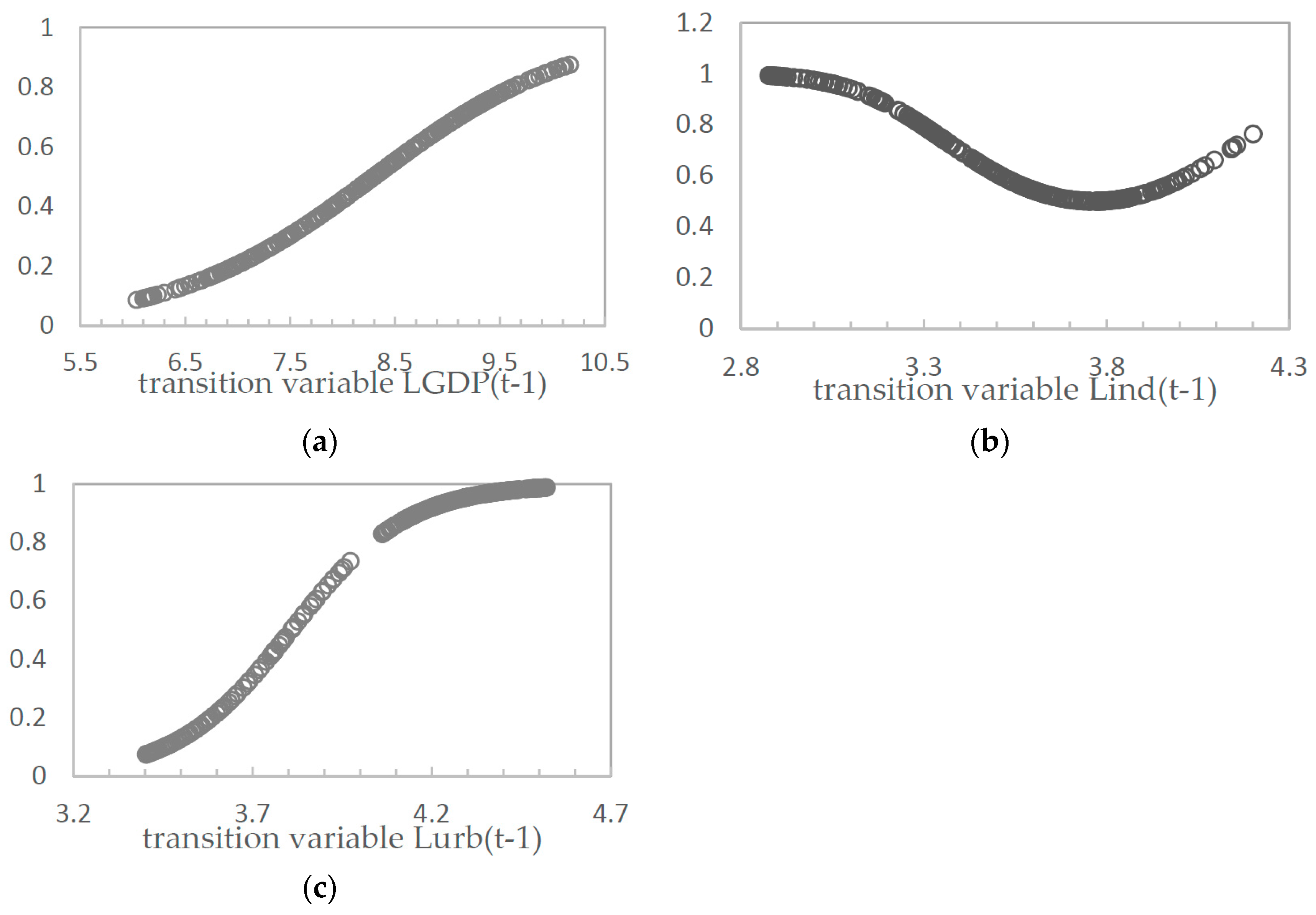
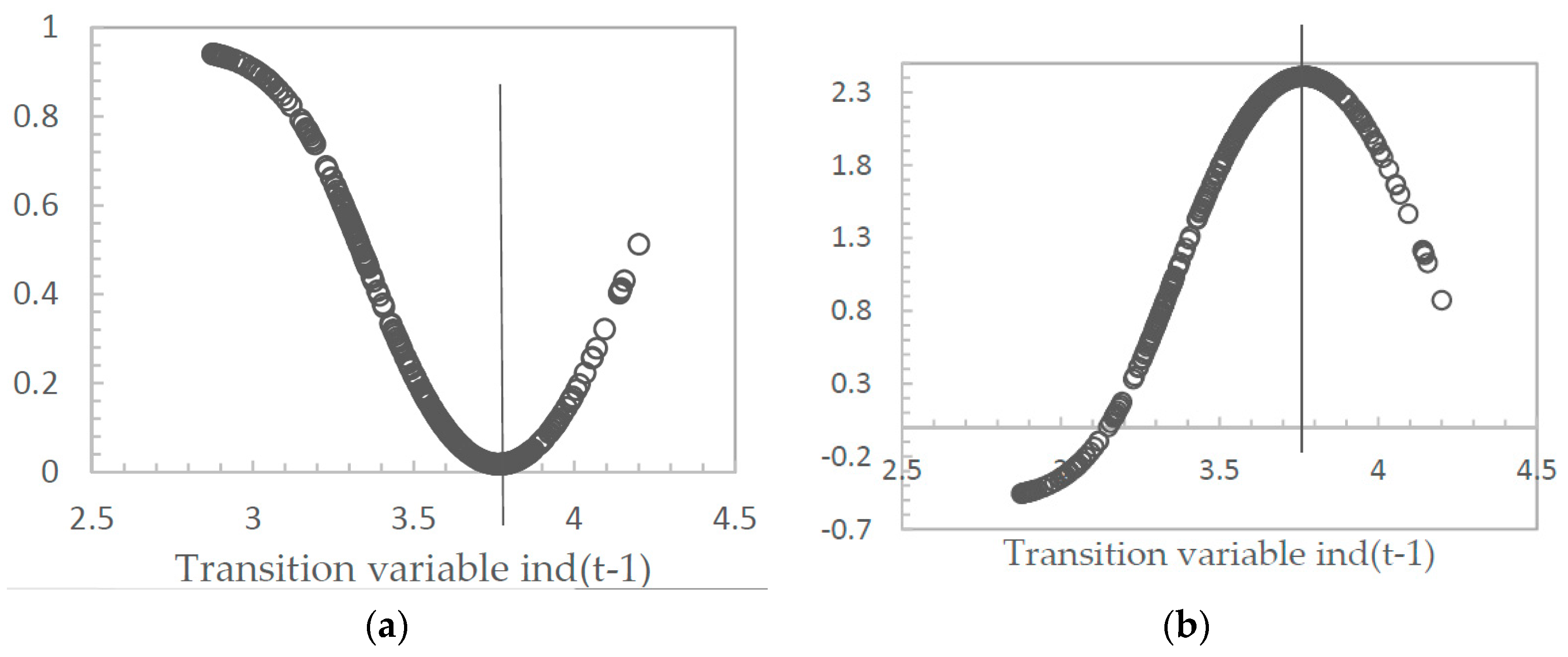
First, the empirical results show that evidence reported for a nonlinear relationship among natural gas consumption, GDP per capita, industrialization and urbanization. Such a nonlinear result may be the reason why existing studies on natural gas consumption, economic growth and industrial development appear to give diverse results. Results from three nonlinear models where the optimal model uses industrialization as transition variable, implying that the influence of industrialization on natural gas consumption of current emerging economies is non-negligible.

Second, specifying GDP per capita, industrialization and urbanization as transition variables, the threshold level of system transformation is US $4,023.8, 43.2% and 45.1%, respectively. Before and after the turning point, the effect of per capita GDP on natural gas consumption is relatively complex. When the transition variable is itself, the effect on natural gas consumption is promoting in the two regimes; when industrialization is adopted as the transition variable, influence effects range from inhibition to promotion, and the effects are relatively small comparing with another influential factors generally. When the transition variable is urbanization, influence effects range from promotion to suppression. The impacts of industrialization on natural gas consumption are from promotion to suppression in three PSTR models, which means that industrial transformation and upgrading can save energy, and that industrialization is also a major factor impacting natural gas consumption from estimated coefficients. The influence of urbanization on natural gas consumption is always to promote, which suggests that urbanization will bring huge gas consumption and its growth is rigid.

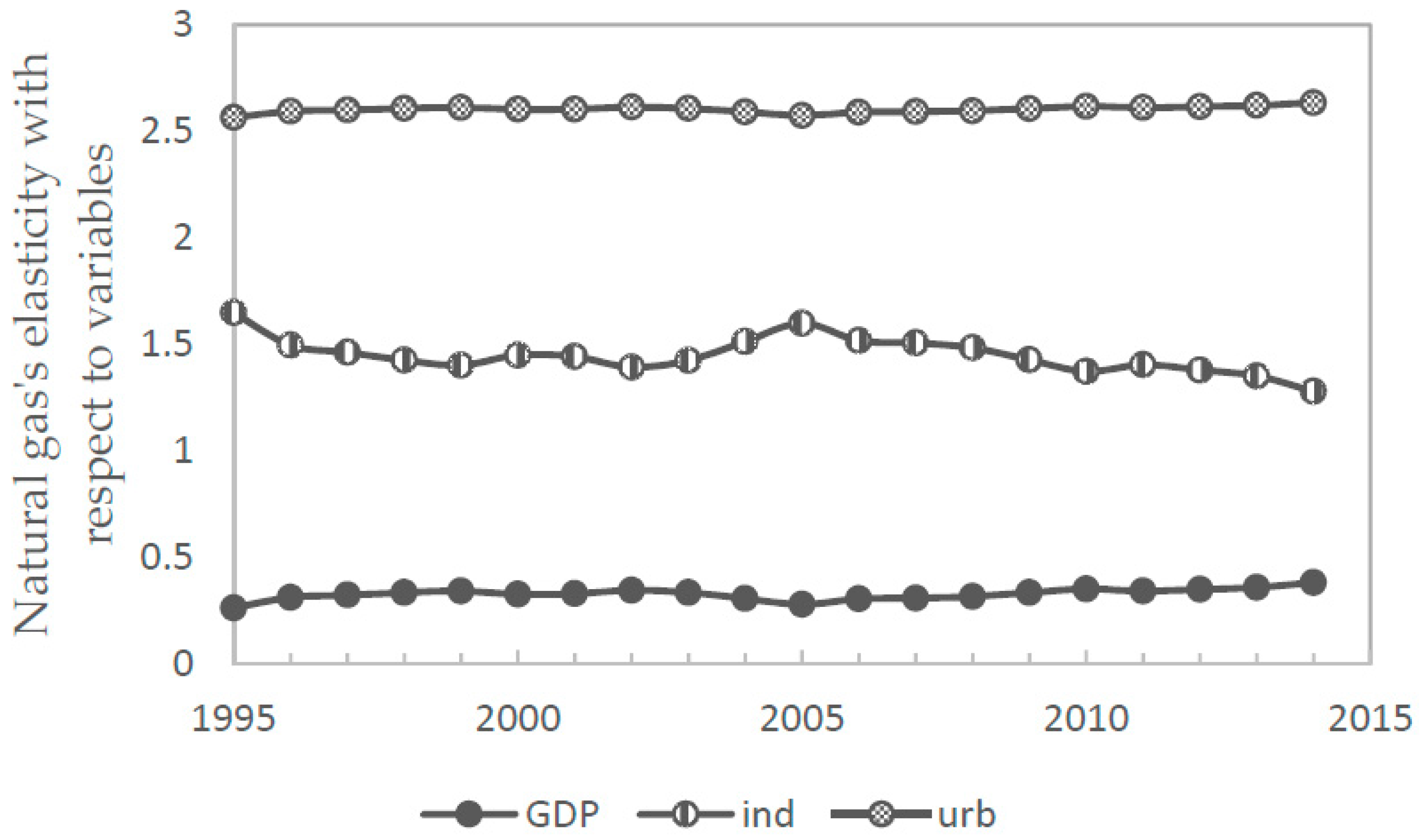
Third, the estimated elasticities of the time dynamic suggest that natural gas consumption has inelastic GDP per capita, elastic industrialization, and elastic urbanization. Moreover, the elasticity of GDP per capita fluctate and rise generally as time goes by, which may be because emerging economies are still in economic transformation and upgrade stages, and economic development promotes not natural gas consumption specifically but gross energy consumption, implying that economic development costs energy consumption, but this study obtains that natural gas consumption is insensitive to the change of GDP per capita. The elasticity of industrialization tends to fall with fluctuations, which is because both the dual pressure from industrial transformation and upgrade, energy saving and emissions reduction and technological advancement inhibit energy consumption, inclusive of natural gas consumption, when industrial development reaches a certain level. The elasticity of urbanization shows linear and stability features at a high level over time, because natural gas consumption is mainly for civil use, and the consumption of household energy is normally rigid, and its contribution to natural gas consumption is large under the pull of urbanization.

Forth and finally, according to the regional difference analysis for 16 emerging economies, the results show that an influential effect on natural gas consumption exists with significant regional difference during economic development. Most of these countries are in the first regime of the industrialization level, and in this regime the promotion effect of GDP per capita on natural gas consumption gradually weakens. The influence of industrialization on natural gas consumption turns from negative to positive, and then this promotion becomes further strengthened with the progress of industrialization.

The findings suggest that any factor of natural gas consumption changes cause structural change of the relationships among natural gas consumption, GDP per capita, industrialization and urbanization rate. According to the above research, we can provide the following beneficial conclusions for the sustainable development of emerging economies. Firstly, under the environment of global economic downturn and coexisting energy shortage problem, the industry upgrading and transformation strategy for emerging economies is the engine of economic development and also plays an important role in saving energy. Secondly, regardless of which stage the countries are in, the development of urbanization may make natural gas consumption under pressure of accelerated growth in the future. While the increase of natural gas consumption is the embodiment of the energy consumption structure optimization, on the other hand, countries should be prepared for changes to the natural gas supply in the development of urbanization. Thirdly, countries should focus on the complex relation between natural gas consumption and per capita GDP in different transition variables, and develop relevant strategies according to their own development policy and development stage properly. Lastly, the most important is that each country should not ignore the “threshold effect” between industrialization and natural gas consumption, and the structural change caused by the transition variable of industrialization should be taken into full account when analyzing and forecasting the natural gas consumption of emerging economies. Moreover, policy-makers should not neglect such nonlinear relationships of natural gas consumption before taking any measurements about economic development and sustainable development.

References

1. Kum, H.; Ocal, O.; Aslan, A. The relationship among natural gas energy consumption, capital and economic growth: Bootstrap-corrected causality tests from G-7 countries. Renew. Sustain. Energy Rev. 2012, 16, 2361–2365. [Google Scholar] [CrossRef]
2. Apergis, N.; Payne, J.E. Energy consumption and economic growth: Evidence from the Commonwealth of Independent States. Energy Econ. 2009, 31, 641–647. [Google Scholar] [CrossRef]
3. Shahbaz, M.; Lean, H.H.; Farooq, A. Natural gas consumption and economic growth in Pakistan. Renew. Sustain. Energy Rev. 2013, 18, 87–94. [Google Scholar] [CrossRef] [Green Version]
4. Işik, C. Natural gas consumption and economic growth in Turkey: A bound test approach. Energy Syst. 2010, 1, 441–456. [Google Scholar] [CrossRef]
5. Wei, B.R.; Yagita, H.; Inaba, A.; Sagisaka, M. Urbanization impaction energy demand and CO2 emission in China. J. Chongqing Univ. Eng. 2003, 5, 46–50. [Google Scholar]
6. Parikh, J.; Shukla, V. Urbanization, energy use, and greenhouse effects in economic development: Results from a cross-national study of developing countries. Glob. Environ. Chang. 1995, 5, 87–103. [Google Scholar] [CrossRef]
7. Imai, H. The effect of urbanization on energy consumption. J. Popul. Probl. 1997, 53, 43–49. [Google Scholar]
8. Jones, D.W. Urbanization and energy. Encycl. Energy 2004, 6, 329–335. [Google Scholar]
9. Lariviere, I.; Lafrance, G. Modelling the electricity consumption of cities: Effect of urban density. Energy Econ. 1999, 21, 53–66. [Google Scholar] [CrossRef]
10. Ewing, R.; Rong, F. The impact of urban form on U.S. residential energy use. Hous. Policy Debate 2008, 19, 1–30. [Google Scholar] [CrossRef]
11. Zamani, M. Energy consumption and economic activities in Iran. Energy Econ. 2007, 29, 1135–1140. [Google Scholar] [CrossRef]
12. Jiang, Z.; Lin, B. China’s energy demand and its characteristics in the industrialization and urbanization process. Energy Policy 2012, 49, 608–615. [Google Scholar]
13. Wang, T.; Lin, B. China’s natural gas consumption and subsidies—From a sector perspective. Energy Policy 2014, 65, 541–551. [Google Scholar] [CrossRef]
14. Kani, A.H.; Abbasspourb, M.; Abedi, Z. Estimation of demand function for natural gas in Iran: Evidences based on smooth transition regression models. Energy Model. 2014, 36, 341–347. [Google Scholar] [CrossRef]
15. Aslan, A. Does natural gas consumption follow a nonlinear path over time? Evidence from 50 US States. Renew. Sustain. Energy Rev. 2011, 15, 4466–4469. [Google Scholar] [CrossRef]
16. Fallahi, F. Causal relationship between energy consumption (EC) and GDP: A Markov switching (MS) causality. Energy 2011, 36, 4165–4170. [Google Scholar] [CrossRef]
17. Moral-Carcedo, J.; Vicens-Otero, J. Modelling the non-linear response of Spanish electricity demand to temperature variations. Energy Econ. 2005, 27, 477–494. [Google Scholar] [CrossRef]
18. Zhao, J.; Fan, J. Empirical research on the inherent relationship between economy growth and energy consumption in China. Econ. Res. 2007, 8, 31–42. (In Chinese) [Google Scholar]
19. He, X.; Pan, H. Nonlinear relationship between energy consumption and economic growth: Evidence from PSTR approach. China Popul. Resour. Environ. 2013, 23, 84–89. (In Chinese) [Google Scholar]
20. Lee, C.C.; Chiu, Y.B. Electricity demand elasticities and temperature: Evidence from panel smooth transition regression with instrumental variable approach. Energy Econ. 2011, 33, 896–902. [Google Scholar] [CrossRef]
21. Bessec, M.; Fouquau, J. The non-linear link between electricity consumption and temperature in Europe: A threshold panel approach. Energy Econ. 2008, 30, 2705–2721. [Google Scholar] [CrossRef]
22. Sadorsky, P. Renewable energy consumption and income in emerging economies. Energy Policy 2009, 37, 4021–4028. [Google Scholar] [CrossRef]
23. Sadorsky, P. The impact of financial development on energy consumption in emerging economies. Energy Policy 2010, 38, 2528–2535. [Google Scholar] [CrossRef]
24. Asif, M.; Muneer, T. Energy supply, its demand and security issues for developed and emerging economies. Renew. Sustain. Energy Rev. 2007, 11, 1388–1413. [Google Scholar] [CrossRef]
25. Liu, Y.; Chen, S.; Zhang, Y.; Zou, X.; Wang, Y. Energy Kuznets curve: Evidence from developed countries. Chin. J. Manag. Sci. 2008, 16, 648–653. (In Chinese) [Google Scholar]
26. Richmond, A.K.; Kaufmann, R.K. Is there a turning point in the relationship between income and energy use and/or carbon emissions? Ecol. Econ. 2006, 56, 176–189. [Google Scholar] [CrossRef]
27. Duarte, R.; Pinilla, V.; Serrano, A. Is there an environmental Kuznets curve for water use? A panel smooth transition regression approach. Econ. Model. 2013, 31, 518–527. [Google Scholar] [CrossRef]
28. Jones, D.W. How urbanization affects energy-use in developing countries. Energy Policy 1991, 19, 621–629. [Google Scholar] [CrossRef]
29. Northam, R.M. Urban Geography; John Wiley & Sons: Hoboken, NJ, USA, 1979. [Google Scholar]
30. González, A.; Teräsvirta, T.; Dijk, D. Panel Smooth Transition Regression Models; University of technology Sydney: Brisbane, Australia, 2005. [Google Scholar]
31. Fouquau, J.; Hurlin, C.; Rabaud, I. The Feldstein–Horioka puzzle: A panel smooth transition regression approach. Econ. Model. 2008, 25, 284–299. [Google Scholar] [CrossRef]
32. Dijk, D.; Teräsvirta, T.; Franses, P.H. Smooth transition autoregressive models—A survey of recent developments. Econ. Rev. 2002, 21, 1–47. [Google Scholar] [CrossRef]
33. Granger, C.W.J.; Terasvirta, T. Modelling Non-Linear Economic Relationships; Oxford University Press: Oxford, UK, 1993. [Google Scholar]
34. Teräsvirta, T. Specification, estimation, and evaluation of smooth transition autoregressive models. J. Am. Stat. Assoc. 1994, 89, 208–218. [Google Scholar]
35. Hansen, B.E. Threshold effects in non-dynamic panels: Estimation, testing, and inference. J. Econom. 1999, 93, 345–368. [Google Scholar] [CrossRef]
36. Gao, T. Panel data model. In Econometric Analysis Method and Modeling; Tsinghua University Press: Beijing, China, 2009. (In Chinese) [Google Scholar]
37. Colletaz, G.; Hurlin, C. Threshold Effects of the Public Capital Productivity: An International Panel Smooth Transition Approach. Available online: https://halshs.archives-ouvertes.fr/halshs-00008056/document (accessed on 24 October 2016).
38. Hoskisson, R.E.; Eden, L.; Chung, M.L. Strategy in Emerging Economies. Acad. Manag. J. 2000, 43, 249–267. [Google Scholar] [CrossRef]
39. Liu, X. Analysis for economic growth and energy. Appl. Stat. Manag. 2006, 4, 443–447. (In Chinese) [Google Scholar]
40. Sun, H.; Cheng, J. China energy demand forecast and analysis in the process of industrialization and urbanization. China Popul. Resour. Environ. 2011, 7, 7–12. (In Chinese) [Google Scholar]
41. Tian, C.; Hao, Y. Compare and review of emerging economies and their difference. Comp. Econ. Soc. Syst. 2011, 5, 118–125. (In Chinese) [Google Scholar]
Figure 1. Transition function of threshold variables, list as: (a) Transition function of L G D P ( t 1 ) is contained in the first panel; (b) Transition function of L i n d ( t 1 ) contained in the second panel; (c) Transition function of L u r b ( t 1 ) contained in the third panel.
Sustainability 08 01089 g001
Figure 2. Natural gas’s elasticity with respect to variables.
Sustainability 08 01089 g002
Figure 3. Natural gas consumption’s elasticity with respect to variables in different regimes using i n d ( t 1 ) as transition variable are listed as: (a) Natural gas consumption with respect to GDP per capital is contained in the first panel; (b) Natural gas consumption with respect to industrialization contained in the second panel.
Sustainability 08 01089 g003