Article

A Vector Auto Regression Model Applied to Real Estate Development Investment: A Statistic Analysis

1
School of Management, China University of Mining & Technology, Xuzhou 221116, China
2
Department of Economics, Ritsumeikan University, Kusatsu 525-8577, Japan
3
Department of Electrical, Electronic & Computer Engineering, University of Pretoria, Pretoria 0002, South Africa
4
College of Economics and Management, Northwest A & F University, Yangling 712100, China
5
UNSW Australia, Sydney 2052, Australia
*
Author to whom correspondence should be addressed.
Sustainability 2016, 8(11), 1082; https://doi.org/10.3390/su8111082
Submission received: 20 August 2016 / Revised: 10 October 2016 / Accepted: 18 October 2016 / Published: 25 October 2016
(This article belongs to the Section Sustainable Engineering and Science)

Abstract

:
This study analyzes the economic system dynamics of investment in real estate from mainly four participants in China. Local governments limit the supply of commercial and residential land to raise fiscal revenue, and expand debts by land mortgage to develop industrial zones and parks. Led by local government, banks and real estate development enterprises forge a coalition on real estate investment and facilitate real estate price appreciation. The above theoretical model is empirically evidenced with VAR (Vector Auto Regression) methodology. A panel VAR model shows that land leasing and real estate price appreciation positively affect local government general fiscal revenue. Additional VAR models find that bank credit in addition to private and foreign funds respectively have strong positive dynamic effects on housing prices. Housing prices also have a strong positive impact on speculation from private funds and hot money.

1. Introduction

Since the 1998 reform of the housing institution in China, investment in real estate has increased, particularly since 2003. Investment by real estate development enterprises rose from 361.4 billion RMB in 1998 to 1015.3 billion RMB in 2003, and subsequently sharply increased to 9503.6 billion RMB by 2014 (Data source: China Statistic Yearbooks of 2004 and 2015.). In addition to real estate development enterprises (suppliers), individuals and institutions (customers) also contributed to the real estate investment increase; because of the expectation that there would be a dramatic rise in housing demand, the housing prices accompanying urbanization development also spiked. Real estate was a desirable investment financially because of a lack of investment goods in China. More and more funds from customers were invested in real estate in search of house price appreciation profits, such as the Wenzhou house speculation groups. Such investments, particularly speculative demand, led to an overheated real estate industry thus further boosting the housing price upswing.
There was also excessive investment in real estate in Japan during the 1980s and the United States during the 2000s; however, the Chinese real estate market is unique. The Chinese real estate market behaves differently than the US or UK markets because of differences in the political environment, legal systems, and culture, as Wang and Wang point out [1]. One important difference is that all urban land in China is owned by the state, and local governments have a strong power on the real estate market by controlling land release and granting development rights. Liu et al. [2] state that, in recent years, local governments in China have significantly increased their land development by acquiring land from farmers and leasing it on a large scale to industrial and commercial developers. They argue that local land development has contributed to an investment-driven growth in China that is not sustainable in the long run. Based on panel data covering all provinces from 1998 to 2005, they find that the impact of public land leasing stimulated local fiscal revenue and gross domestic product. Liu et al. [3] also point out that the local state-dominated model of administrative urbanization in China differs markedly from the urban growth model in Western nations. Land-based urban development can rapidly produce dramatic economic and urban outcomes, but whether these are beneficial to the urban and rural residents is not clear. Both the investment-driven growth of Liu et al. [2] and the administrative urbanization of Liu et al. [3] are based on land and are led by local government. It seems that local government-led land-based investment or development accompanying urbanization drove growth in China. Lai [4] asserts that there was very excessive infrastructure and real estate investment in China from 2003 because of the inappropriate growth strategy. Under this complex and unique context, it is relevant to discuss how funds are invested in real estate, and the leading role of local government in the process. Various studies have discussed the importance of local government in land leasing; however, most do not clearly distinguish and connect the “land fiscal revenue” and “land finance” of local government, and are limited to descriptive analysis. This paper will clarify the “land fiscal revenue” and “land finance” process of local government by institutional analysis and then empirically evidence it.
In addition to the state-owned land system, other unique characteristics contribute to the high investment in the real estate industry. Cary [5] asserts that the revenue sharing system, a weak banking framework and the lack of investment opportunities also drove the overheated economy in China. Zhang and Sun [6] point out that the real estate situation included risks of real estate credit exposure, government guarantees, and maturity mismatches and suggested advancing banking reform, encouraging local government rationality and strengthening the regulation of foreign capital flows in and out of the Chinese real estate industry. Hence, besides local government, the banking sector, the private sector (individuals), and the foreign sector all played important roles. The banking sector provides loans to the local government, real estate development enterprises and individuals, while the private sector and foreign sector funds speculate on real estate. As Su and Tao [7] highlight, the financial ties between local governments, real estate developers, and banks that share the common goal of city expansion have forged a strong growth coalition in China’s local landscape. Thus, it is worth studying the various roles of different participants in the process of investment in real estate. Some studies [8,9,10,11] discuss the influence of bank credit and foreign funds on housing prices in China; however, how these funds are invested in real estate is not fully known and there are few empirical studies on the effect of private funds (funds from individuals) on housing prices. Thus, this paper is a tentative study in this field.
If housing prices decrease, local governments will be trapped in a serious debt crisis, and banks, real estate enterprises, and speculations from private and foreign sectors that withdraw late from the market would face huge losses. The situation in China at present is very similar to developments in 1980s Japan—a very risky and unsustainable position. This paper aims to address some urgent issues that have not yet been clearly studied. How are funds being invested in real estate? What roles do the different economic participants play in this process, particularly the leading role of local government? What are their influences on housing prices? By studying these issues, this paper tries to clarify different investments in real estate and thus understand speculative demand, and propose some policy suggestions by testing the efficiency and effectiveness of current local government development strategies. As Wang and Wang [1] emphasize, China is an ideal laboratory to study the influence of speculative demand versus fundamentals on property prices.
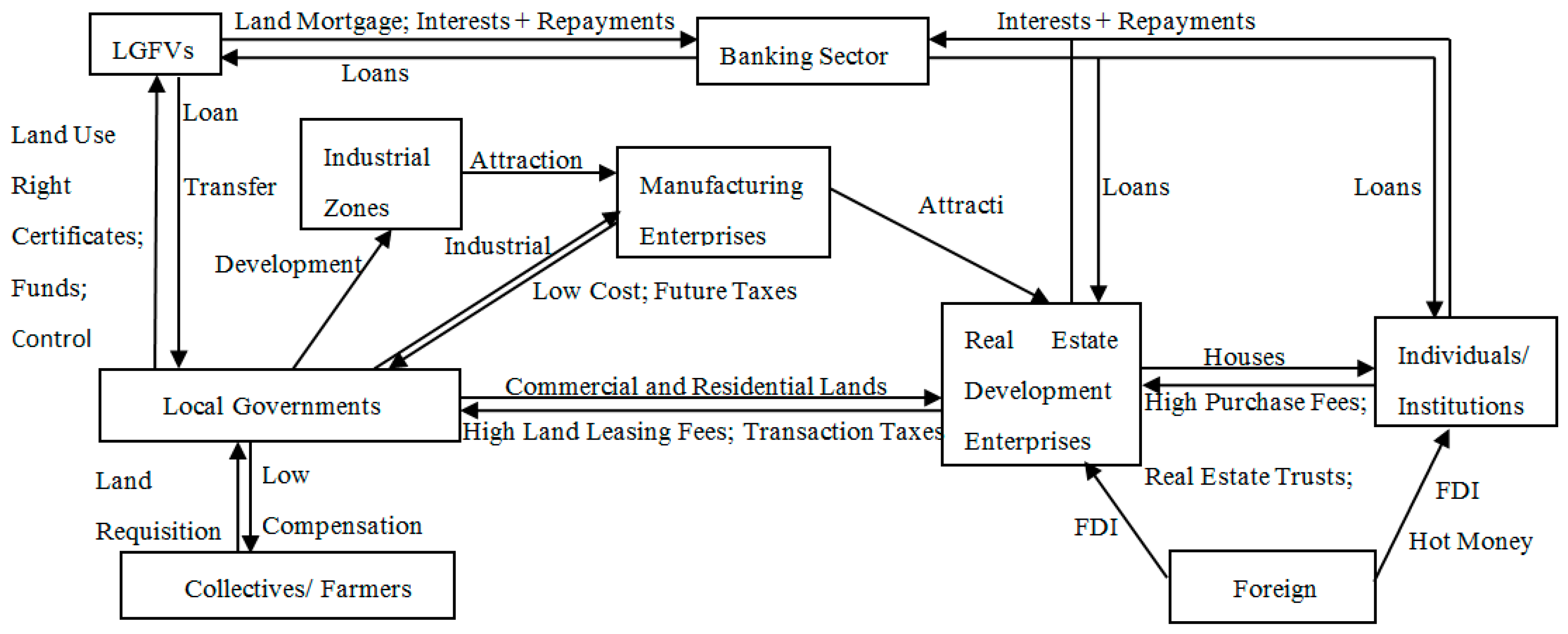
Section 2 analyzes the process of local government-led investment-driven growth in real estate prices. The roles of local governments, the banking sector, real estate development enterprises, individuals, and the foreign sector are discussed. Based on the theoretical model of real estate investment explained in Section 2, Section 3 empirically tests the role of local government in real estate investment and thus housing prices by a panel VAR model, and analyzes the dynamic effects of different investment types on housing prices by three other VAR models. Section 4 outlines conclusions.

2. Local Government-Led Investment in Real Estate

2.1. Local Governments

In China, urban land is state owned, whereas rural land is owned by collectives. It is noteworthy that the proprietary rights of land as well as the buildings on it are separated in China and that properties can be privately owned by individuals and institutions. According to the Land Administration Law promulgated in 1998, collective-owned land is first converted into state-owned land through land acquisition by the local government before being developed for infrastructural, industrial, or commercial purposes. Thus, collectives (the owners of rural land) are unable to transfer their land rights privately for urban use, and only get a low compensation for land acquisition by the local government. Generally, local government unilaterally sets a low compensation level that is much less than the leasing price of the land in commercial markets [12].

2.1.1. Land Revenue

Table 1 shows local government overall financial revenues and those directly attributable to land from 2001 to 2012. The taxes directly related to land increased from 49.8 billion RMB in 2001 to 1012.8 billion RMB in 2012, giving general budgetary revenue ratios of 6.4% and 16.6%, respectively. Land leasing revenues also rose sharply from 179.4 billion RMB in 2001 to 3702.8 billion RMB in 2012. Taking land taxes and leasing revenues together as a ratio of total local government revenue (general revenue + extra-budgetary revenue) shows a drastically increasing ratio from 15.3% in 2001 to 73.9% in 2010, before dropping somewhat to 60.6% by 2012. Other indirect land tax revenues are not considered here; hence the real income from land was even higher [7]. This implies that local governments rely on land leasing for revenue.
Local governments lease land to real estate developers in four ways: negotiation (xieyi), tender (zhaobiao), auction (paimai), and listing (guapai). Negotiation means land users and the local government negotiate the leasing terms through a one-to-one discussion. Tenders are organized publicly, where land users state their leasing terms and the government selects one based on a comprehensive consideration rather than solely on price. Auctions are also public, and the highest bidder obtains the right to use the land. In contrast to an auction, a listing gives land users 10 or more days to quote a price in writing and the floor price is public. Cao et al. [13] found that because of fierce regional competition, local governments lease land to the manufacturing sector mainly by negotiation, at a low price or even with a subsidy. Commercial and residential projects are mainly leased through tender and auction, and local governments limit land supply through their underlying institutions, municipal land management and reserve centers to raise the leasing price. The Ministry of Land and Resources of the People’s Republic of China [12] states that the overall land leasing price for commercial use in 105 major cities in 2011 was 5654 RMB/sq·m, followed by residential purposes at 4518 RMB/sq·m, while industrial use was only 652 RMB/sq·m. Table 2 shows industrial, commercial, and residential land supplies from 2003 to 2011. The greatest amount of land supplied by local governments was for industrial purposes, increasing from 99,435.0 ha in 2003 to 191,314.5 ha in 2011. Residential land supplies ascended from 43,323.3 ha in 2003 to 126,452.9 ha in 2011, followed by commercial land. Notably, industrial land supply accounted for 50% or more of total supply, significantly greater than the residential and commercial ratios. Hence, with its monopoly on local land supply, the local government is incentivized to increase industrial land supply to raise future tax revenue and stimulate local economic development and thus commercial and residential land demand. At the same time, it limits the land supply for residential and commercial projects to increase current land leasing revenues. With the different strategies of land supply to different sectors, local government tries to optimize revenue as well as economic and thus political advantages based on its monopolistic power on land supply [2,7,13,14,15,16].

2.1.2. Land Finance

In addition to revenues from land, local states make full use of their land ownership to obtain loans through land mortgage, known as land finance. The 1995 budget law banned local governments from issuing bonds directly; hence, they set up local government financing vehicles (LGFVs) to borrow money from banks [13]. These LGFVs include urban development companies, land banking centers and state-owned asset management centers. Land mortgage is the most common way for local governments to get LGFV loans. The general procedure for this is that land administrative departments define the purpose and term of banking land according to government planning, and issue land use right certificates to the land banking centers. With these certificates, land banking centers can either directly apply for bank loans or indirectly collateralize loans borrowed by other LGFVs. Table 3 shows recent local government debts by type. Local governments have high debt levels, increasing from 10,717.5 billion RMB in 2010 to 17,890.9 billion RMB by June 2013. Repayment obligations accounted for approximately 61% of total debt from 2010 to June 2013. Local governments guaranteed 21.8% and 14.9% of the total debts in 2010 and June 2013, respectively. Table 4 illustrates the amounts and ratios of local government debt through LGFVs and banks, and highlights those used for infrastructure projects in recent years. Debts financed through LGFVs are high, at 46.4% in 2010 and 39.0% in June 2013. With the increase in land leasing price, banks consider land as prime collateral, and provide many loans to local governments. Local government bank debts were 79.0% in 2010 and 56.5% in June 2013. Using these loans, local governments develop industrial zones and expand infrastructure. Local government infrastructure debts were 89.4% in 2010 and 88.6% in June 2013. The construction of industrial zones and parks helps attract investment and thus promotes the local industrial and commercial development level, further elevating land-related taxes and commercial land values.

2.2. Real Estate Development Enterprises

As suppliers to the housing market, real estate development enterprises are important industry players. Table 5 shows the 1999–2012 fund components raised by real estate development enterprises: “others” account for 46.55% of total funds, followed by “self-raised funds” (32.01%) and “domestic loans” (19.93%). “Domestic loans” are mainly the real estate development loans of financial institutions. Moreover, “others” and “self-raised funds” include significant mortgage loans from buyers [13]. Thus, real estate development enterprise funding mainly came from banks. Real estate development investment increased in conjunction with total fund growth, at a rate surpassing 30% in 2003, 2007 and 2010. This suggests that real estate development enterprises drastically expanded their investments in real estate in recent years. Land purchase fees accounted for approximately 20% of real estate development investments, implying that land cost is large and translated into high housing price. Moreover, real estate development enterprises try to further raise the housing price level to increase their profits, since the seller is more powerful than the buyer in Chinese housing market. According to the National Bureau of Statistics of China [18], units of housing completed is lower than those sold since 2005, and the ratio of units completed to sold in 2014 was still at a high level of 1.3. Thus, real estate tends to be a seller’s market in China.

2.3. The Banking Sector

The Chinese financial system is bank based and, as a capital-intensive industry, the real estate industry is closely connected with the banking sector. The analysis in Section 2.1 and Section 2.2 shows that both local governments and real estate development enterprises rely heavily on banks for their development funds. The Specialized Statistical Analysis Team of China Banking Regulatory Commission [19] declares that approximately 60% of real estate industry funding comes from banks. With the high level of liquidity and the increase in housing prices, the banking sector expanded loans to the real estate industry from 2003. As shown in Table 6, total outstanding deposits rose from 208,055.6 billion RMB in 2003 to 917,368.1 billion RMB in 2012, with an average annual growth rate of 19.3% in the 2000s, suggesting massive liquidity in the banking sector. Banks tended to choose real estate as a primary investment target. Outstanding loans to the real estate industry increased from 1840 billion RMB in 2003 to 12,100.0 billion RMB in 2012, and accounted for an increasing percent of total outstanding loans, from 11.57% in 2003 to 19.2% to 2012. Both real estate development enterprises and consumers get a large number of bank loans. Real estate development outstanding loans increased from 660 billion RMB in 2003 to 3863 billion RMB in 2011, while house purchase outstanding loans ascended from 1180 billion RMB in 2003 to 8237 billion RMB in 2011. Thus, there is an expansion of bank credit to real estate that causes upswings in housing prices [8].

2.4. The Foreign Sector

With the increase in housing prices, the foreign sector expanded their investment in the real estate industry. The People’s Bank of China [20] shows that there are four ways foreign funds enter the real estate market: (1) directly establishing real estate development enterprises or sharing the equity of domestic enterprises; (2) indirect investment in the bond market or through foreign-funded real estate intermediary enterprises by volume purchase of real estate and subsequently selling land for retail purposes; (3) foreign banks providing loans to real estate enterprises and consumers; (4) non-resident foreign exchange inflows purchasing houses after exchange settlement. Of these, (1), the second part of (2); and (3) are included in foreign direct investment (FDI); while (4) is considered “hot money”. Table 7 shows FDI, FDI to the real estate industry, and hot money net flows from 2000 to 2012. All three variables started to rapidly increase around 2003. FDI flows increased from $53.3 billion US dollars (USD) in 2003 to $116.0 billion USD in 2011. FDI in real estate increased as a percent against overall FDI, from 9.8% ($5.2 billion USD) in 2003 to 21.6% ($26.9 billion USD) in 2011. During 2004–2011, there was a large net inflow of hot money to China, reaching peaks of $76.8 billion USD in 2004 and $77.1 billion USD in 2010. This foreign investment in real estate has contributed to rising housing prices [9,10,11].

2.5. Individuals

The Bank of Japan [21] points out that, in addition to bank credit, real estate market funding can come from individuals, corporate legal persons and foreign funds through real estate funds and other means. With the expectation of housing price appreciation, individuals in China consider real estate as a best investment asset. They can invest in real estate directly by purchasing it, or indirectly through the securities market and real estate trust products. Chinese real estate trusts are different from Real Estate Investment Trusts (REITs), and there are no genuine ones in China. The present real estate trust products in China are mainly issued by bond, where fund flow is similar to bank credit, and the real estate trust plays a role as a second bank. Funds collected through real estate trust products from individuals mainly flow into real estate development enterprises that mortgage their real estate development projects to the trust. The Wenzhou group of house speculation [22] and the high vacancy rate (i.e., the ratio of “houses already being sold but are still vacant/the total houses already being sold. This differs from Western countries that include houses not yet sold. Thus, high vacancy rate in China shows that individuals purchase housing for speculation rather than living, which is another evidence of high investment to real estate from individuals) of houses [23] have been cited in many studies as examples of direct investment by individuals. Table 8 illustrates that areas sold and sales of commercial houses rose drastically from 2003 to 2012, with the exception of 2008 in the midst of the global financial crisis. Sales increased almost eight-fold, from 795.5 billion RMB in 2003 to 6445.6 billion RMB in 2012. Individuals’ indirect investment also increased, with the value of issued real estate trust products sharply ascending from 81.4 billion RMB in 2003 to 3156.4 in 2011, particularly in 2010 when there was a 335.3% growth (see Table 8).

2.6. The Process of Local Government-Led Investment in Real Estate

Section 2.1, Section 2.2, Section 2.3, Section 2.4 and Section 2.5 discussed the roles different participants have in real estate investment. Local governments acquire land from collectives at an extremely low price. They then take advantage of their land supply monopoly and provide lands to the industrial sector at a low price or with a subsidy. At the same time, they undersupply commercial and residential lands to stimulate leasing prices, thereby increasing the revenue as well as economic and thus political profits (land revenue). Through their underlying LGFVs, they expand their bank debts by land mortgage (land finance) for infrastructure construction—such as development of industrial zones and parks—that would attract industrial investment to stimulate local economic development, and thus increase commercial and residential land demand and further raise leasing prices. Since the Chinese real estate industry is a seller’s market, real estate development enterprises translate expensive land costs into high housing prices and further raise housing prices to increase their profits. The foreign sector and individuals also increasingly invest in real estate with expectations of housing price appreciation. In this process, with massive liquidity, the banking sector considers real estate as prime collateral and expands loans to local governments and real estate development enterprises as well to gain profits. Briefly, local governments foster an investment coalition where they, together with real estate development enterprises and banks, develop real estate and aim to raise real estate prices. Speculation from the foreign sector further increases housing prices. This process is summarized in Figure 1.

3. Empirical Test

Section 2 analyzed local government-led investment in real estate, and the roles of different participants in the process. To further grasp the importance of each participant, this section will empirically examine their effects on housing prices.

3.1. Data and Methodology

3.1.1. Data

With respect to local government-related variables, because of the lack of high frequency time series (quarterly or monthly) data, this study collected annual panel data for the 31 provinces/autonomous regions in China from 2003 to 2011 to fulfill empirical analysis. The area of land leased (AL) is used as a proxy of local governments’ land leasing level. Local government general fiscal revenue (GR) represents the fiscal revenue level, where extra-budgetary revenue is excluded. Since all leasing fees enter into extra-budgetary revenue, both are certainly positively connected and there is no need to include extra-budgetary revenue in the empirical analysis. The average commercialized building price (AP) in each province or autonomous region is adopted for the housing price level. These variables are expressed in logarithmic form and expressed as LAL, LGR and LAP, respectively. All the data are from [12,17,18].
Panel provincial data are unavailable for funds-related variables, such as real estate development loans, housing purchasing loans, real estate trust products, and hot money; thus, this paper uses national quarterly time series data from 2003 to 2012 for empirical discussion. The AP is more consistent than the house price index (the method of calculating the housing price index was reformed twice—2005 and 2011—thus there are no consistent successive housing price index data from 2003 to 2012 in China [24]); hence it is adopted to represent the housing price level. Real estate development outstanding loans from financial institutions (DL) and house purchasing outstanding loans (PL) compose the investment in real estate from bank credit. The values of issued real estate trust product (RT) are used as a proxy for private funds invested in real estate as there is no exact data on these. RTs are not only important for the financing of real estate development enterprises, but are also popular with speculative funds from individuals. These are the only data available among private funds invested in real estate. Moreover, there are no exact data for foreign funds invested in real estate, while FDI and hot money (abbreviated as “HM” in the model) are available or countable. Please note that Hot money is a term most commonly used in financial markets to refer to the flow of funds (or capital) from one country to another to earn a short-term profit on interest rate differences and/or anticipated exchange rate shifts. These speculative capital flows are called hot money because they can move very quickly in and out of markets, potentially leading to market instability [25].
Martin and Morrison [25] assert that because hot money flows quickly and is poorly monitored, there is no well-defined method for estimating the amount flowing into a country in a set period. Existing literature mainly uses two methods to approximate the amount of hot money: the direct method, the sum of specific variables that constitute hot money; and the indirect method that captures hot money as a residual of other variables (see Table 9). Because of data limitation in China (The data for “Net flows of non-FDI, non-portfolio investment assets and liabilities held by entities other than the monetary authorities, general government, and banks”, “net flows of non-FDI, non-portfolio investment assets and liabilities held by banks”, and “Portfolio flows” are not available in the International Balance of Payments for China), we cannot follow the direct method of Loungani and Mauro [26], Prasad and Wei [27], and Cheung and Qian [28]. The definitions of “excessive surplus of foreign trade” and “excessive current transfer” developed by Liu [29] are also too comprehensive to identify, whereas the indirect method, “hot money = the change in foreign exchange reserves—foreign trade surplus (or deficit)—net flow of foreign direct investment (FDI)”, is more feasible as data is more readily available. (Please note that Zhang and Shen [30] developed a definition for “normal surplus of foreign trade”, though it remains difficult to identify the “normal” part. The International Balance of Payments Analysis Group of the State Administration of Foreign Exchange [31] approximate annual hot money; however, “investment yield” quarterly data are not available.) However, extant literature on China uses data from different departments to approximate hot money. For example, data on foreign exchange reserves are from the Administration of Exchange Control, on foreign trade surplus are from the Ministry of Commerce, and on FDI are from the Customs Administration. Although, for the same variable, details are distinct across departments. In fact, hot money is a cross-country fund flow, and the International Balance of Payments is the most accurate record of fund inflows and outflows. Therefore, this paper uses quarterly International Balance of Payments from the Finance Institution Database of the Chinese Academy of Social Sciences data to approximate hot money and FDI.
All the above variables are expressed in logarithmic form, seasonally adjusted using the X11 method, and expressed as LDL, LPL, LRT, LFDI and LHM, respectively. Data are sourced from the State Statistical Bureau, the People’s Bank of China, the use-trust network, the Chinese Academy of Social Sciences Database and the Tsinghua Financial Database.
The sample period is from 2003: 2Q–2012: 4Q. The first year is chosen as 2003 because house prices started increasing sharply at that point. Liu [28] finds that the financial reform since 2003 drastically promoted money supply, and thus greatly strengthened the influence of money on house prices. Further, data on loans to the real estate industry have only been available since 2003: 2Q.

3.1.2. Methodology

Sims [35] proposed VARs to conduct a dynamic analysis of a system where changes to a particular variable are affected by changes to other variables, the lags of those variables, and the changes in its own lags. The VAR technique is broadly used in the analysis of financial factors and asset markets [36,37,38,39]. However, the traditional unrestricted VAR has inherent problems. As Pesaran and Shin [38] contend, “the underlying shocks to the VAR model are orthogonalized using the Cholesky decomposition before impulse responses, or forecast error variance decompositions are computed. This approach is not, however, invariant to the ordering of the variables in the VAR”. Consequently, the structural VAR model is developed by Bernanke [40], Blanchard and Quad [41], Sims [42], and Blanchard and Watson [43]. Dekker et al. [36] refer to “imposing a priori restrictions on the covariance matrix of the structural errors and the contemporaneous and/or long-run impulse responses to themselves”. Nevertheless, the number of restrictions positively relates to the number of variables, and it is sometimes difficult to impose a priori assumptions because of complex economic situations. The generalized approach to VAR was advanced by Koop et al. [44] for nonlinear dynamic systems and by Pesaran and Shin [33] for linear systems to overcome the above limitations. It is used in financial problem and real estate market studies, such as Dekker et al. [36], and Ewing and Thompson [45]. Guided by these scholars, this paper uses the generalized VAR technique.
An m-dimensional and p-order vector autoregressive model is presented as follows.
y t = a 0 + i = 1 p Φ i y t i + u t , t = 1 , 2 , ... , T
where y t = ( y 1 t , y 2 t , ... , y m t ) is an m × 1 vector of endogenous variables, jointly determined by its own lags and the lags of other variables. a 0 is a 1 × m vector for the fixed effect, Φ i are m × m coefficient matrices, and u t is an m × 1 matrix of unobserved shocks (disturbances). The matrix form of Φ i is presented below.
Φ i = [ ϕ 11 ( i ) ϕ 12 ( i ) ϕ 1 m ( i ) ϕ 21 ( i ) ϕ 22 ( i ) ϕ 2 m ( i ) ϕ m 1 ( i ) ϕ m 2 ( i ) ϕ m m ( i ) ] , i = 1 , 2 , , p
A panel VAR model has the same structure as a VAR model, in the sense that all variables are assumed to be endogenous and interdependent, but a cross-sectional dimension is added to the representation. A panel VAR of p-order is
y j t = a j 0 + i = 1 p Φ i y j t i + u j t , j = 1 , 2 , ... , N ; t = 1 , 2 , ... , T
where t = 1, 2, …, T is the time index; j = 1, …, N indicates the generic term for the sectional dimension, such as countries, sectors, markets or combinations of these; y j t is an m × 1 vector for section j with m variables; a j 0 is a 1 × m vector for the section-specific; Φ i are m × m coefficient matrices as shown in (2); and u j t is an m × 1 vector of random disturbances.

3.2. Modeling

As Section 2 shows, local governments try to increase their fiscal revenue through disparate land supply strategies for different sectors, and through facilitating the investment in real estate and real estate prices. Therefore, to further examine the relationship between land leasing, local government revenues and housing price levels, a panel VAR model with data for LAL, LGR and LAP in 31 provinces/autonomous regions will be established.
Funds invested in real estate mainly come from the banking sector (bank credit), individuals (private funds), and the foreign sector (foreign funds). Thus, we will establish three VAR models for the three investment types to examine their respective effects on housing prices. We use quarterly time series data since 31 provinces’ panel data for most funds are not available. Series (1) is investment in real estate from bank credit with LDL, LPL and LAP data sets. Series (2) is investment from private funds with LRT and LAP variables. System (3) is investment from foreign funds using LFDI, LHM and LAP.
First, the stationarity of all series is examined. Two tests, the Levin, Lin and Chu test and the PP-Fisher Chi-square test, are applied to the panel data to ensure accuracy (Table 10). All the first difference series DLAL, DLGR, DLAP refuse the null assumption of common unit root (Levin, Lin and Chu test) and that of individual unit root (both tests) at the 1% level. Therefore, the first difference series, DLAL, DLGR, DLAP, enters into the panel VAR model. For the time series data, the augmented Dickey-Fuller (ADF) test is adopted, as shown by Table 11. All the series are I (1) at the 1% level. Thus, their first difference series, DLDL, DLPL, DLRT, DLFDI, DLHM and DLAP, enters into the VAR models.
A panel VAR model and three VAR models are established as follows. For local government-related analysis, the panel VAR consists of the first difference series of DLAL, DLGR, DLAP, with a two-lag length (the principles of LR, FPE and AIC suggest a two-lag length for the panel VAR model.). For fund-related models, bank credit is represented by Model (1), where the first difference series of DLDL, DLPL and DLAP are introduced. Private funds are explained by Model (2), comprised of the first difference series of DLRT and DLAP. Model (3) shows foreign funds and contains the first difference series of DLFDI, DLHM and DLAP. Model (1) hints at a two-lag length, and Model (2) and Model (3) have a one-lag length. The principles of LR, FPE, AIC and HQ hint a two-lag length for VAR models (1). The principles of LR, FPE, AIC, and HQ hint a one-lag length for VAR model (2). The principles of LR, FPE and AIC hint a one-lag length for VAR model (3).
In the panel VAR model,
y i t = [ D L A L i t , D L G R i t , D L A P i t ] , t = 2003 , ... , 2011 ; p = 2
In Model (1),
y t = [ D L D L t , D L P L t , D L A P t ] , t = 2003 Q 2 , ... , 2012 Q 4 ; p = 2
In Model (2),
y t = [ D L R T t , D L A P t ] , t = 2003 Q 2 , ... , 2012 Q 4 ; p = 1
In Model (3),
y t = [ D L F D I t , D L H M t , D L A P t ] , t = 2003 Q 2 , ... , 2012 Q 4 ; p = 1
The panel VAR model and all three VAR models described above are estimated using the EViews 6.0 software and successfully pass the AR root test, implying that they are stable. The impulse response analysis based on the estimated VARs could be used to trace the dynamic responses of each variable to the innovations in a particular variable in the system.

3.3. Results of Impulse Response Analysis

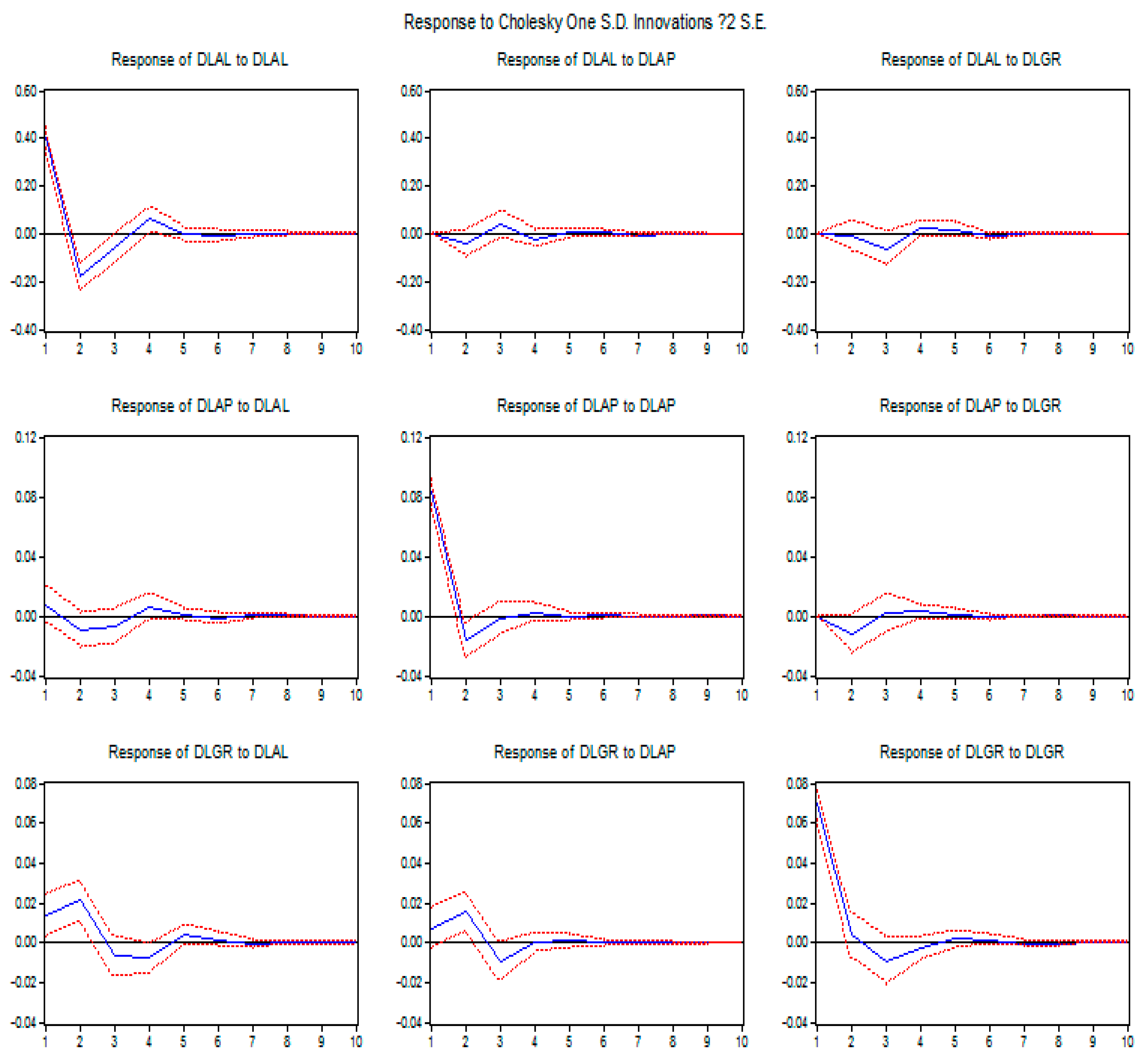
The generalized impulse response functions results of the panel VAR model are illustrated in Figure 2. Following a 1% positive shock to DLAL (A 1% positive shock to “DLAL” or a 1% positive “DLAL” shock means a 1% positive shock in “DLAL”, that is, the one positive standard deviation innovation to the increment of logarithmic “area of land leased”; this holds for a shock to “DLGR”, “DLAP”, “DLDL”, “DLPL”, “DLTR”, “DLFDI” and “DLHM”), the DLGR response peaks at 2.14% in the second period, suggesting that land leasing could promote local government general fiscal revenue. This is consistent with the analysis in Section 2.1 that local governments could increase tax revenue from the manufacturing sector and other land-related revenue through land leasing in budgetary revenue, in addition to land leasing fees. That is why local governments supply industrial land at a low price while limiting the commercial and residential land supply to raise leasing prices. After a 1% positive shock to DLAP, DLGR also responds positively and peaks at 1.77% in the second period. This implies that high housing prices could bring more fiscal revenue to local governments. Thus, local government is strongly incentivized to raise real estate price levels. With a 1% positive shock to DLAL, the DLAP response reaches a peak of −0.93% in the second period, showing that housing price levels would decrease by increasing land supply. Therefore, to raise the real estate price level and thus fiscal revenue, local governments limit the land supply to commercial and residential projects (as discussed in Section 2.1). However, to control high housing prices, a suggested policy option would be to increase land supply.
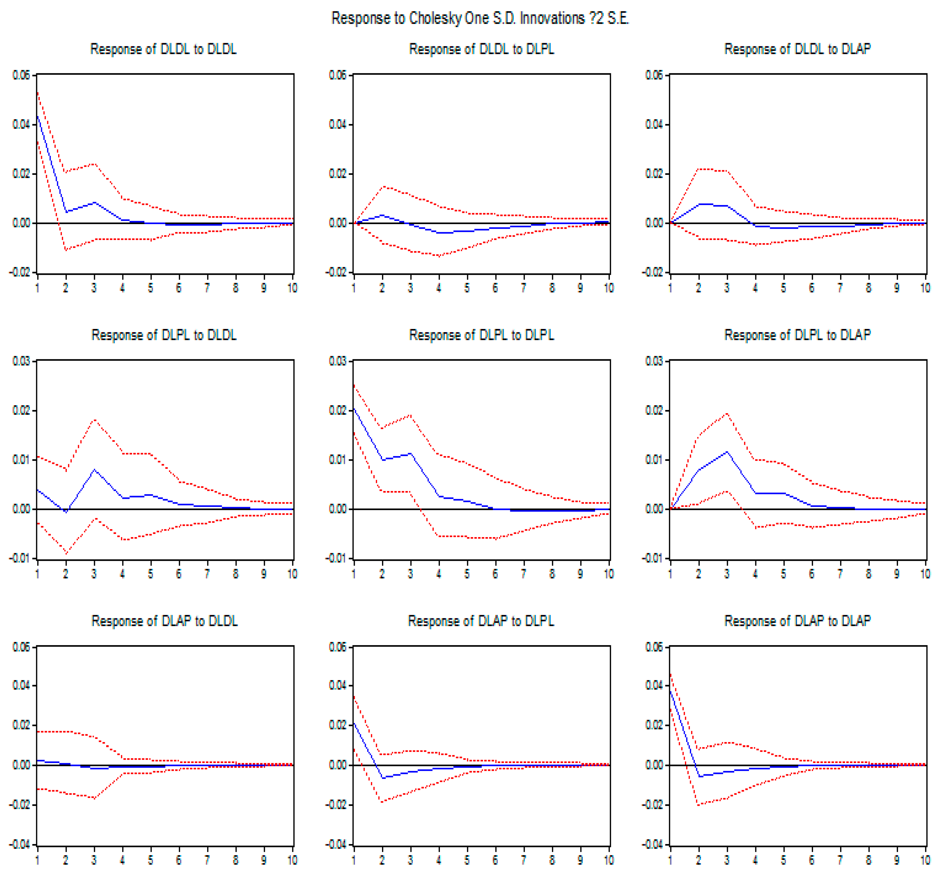
The generalized impulse response functions results of model (1), bank credit, are shown in Figure 3. Following a 1% positive shock to DLDL, DLAP has a very limited response at 0.23% in the first quarter and −0.14% in the third quarter. This suggests that the expansion of bank credit to real estate development enterprises would not decrease housing prices. This is because, in a seller’s market, local governments together with banks and real estate development enterprises forged a coalition to raise investment in real estate and real estate prices, as analyzed in Section 2. When a 1% positive shock to DLPL occurs, DLAP respond at 2.11% in the first quarter, showing that expansion of house purchasing loans could increase the housing demand and thus housing prices.
Both DLDL and DLPL respond positively following a 1% positive DLAP shock, peaking at 0.80% in the second period and 1.57% in the third period, respectively, suggesting that upswings in housing prices encourage the expansion of bank credit to the real estate industry. With an increase in housing prices and high liquidity levels, banks consider real estate as prime collateral and drastically increase loans to the real estate industry.
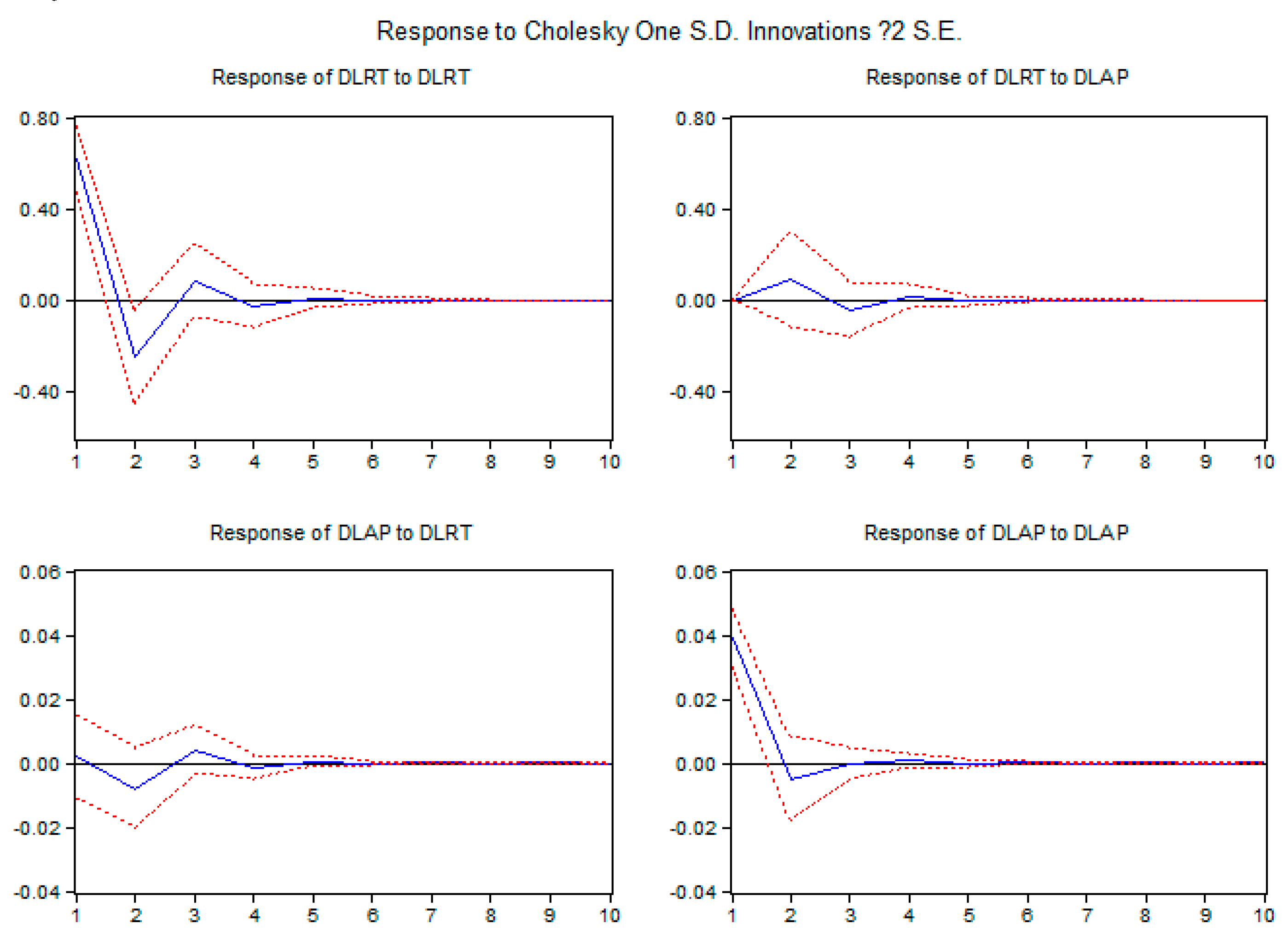
The generalized impulse response functions results of model (2), private funds, are described in Figure 4. The response of DLAP to a 1% positive DLRT shock is greatest at −0.81% in the second quarter, turning to 0.42% in the third quarter. In China, the issued real estate trust products were mainly based on the mortgage of real estate development projects. In other words, after real estate development enterprises mortgage their projects to trusts, the trusts collect funds from individuals by issuing real estate trust products, and these funds indirectly flow to the real estate development enterprises. Therefore, real estate products could help real estate development enterprises obtain funds to increase the housing supply, potentially decreasing housing prices. However, most private funds are used to purchase houses directly by individuals; this could increase the housing demand and thus housing prices.
Interestingly, DLRT peaks at 3.0% in the first quarter following a 1% positive DLAP shock. This illustrates that house price upswings greatly elicit speculation by individuals in real estate trust products, which is consistent with the discussion in Section 2.5.
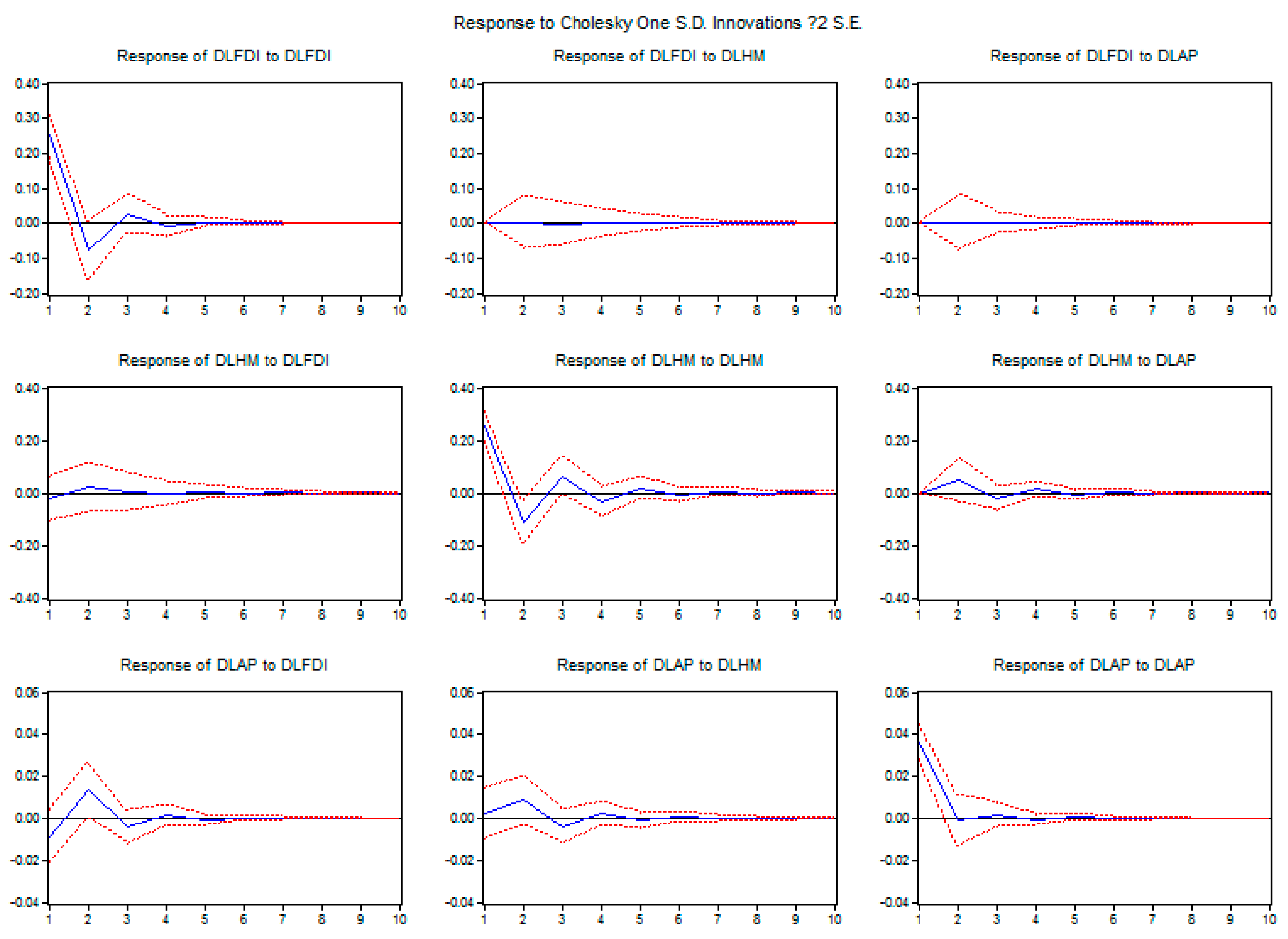
Figure 5 shows the generalized impulse response function results of model (3), foreign funds. When there is a 1% positive shock to DLFDI, the DLAP response peaks at 1.33% in the second quarter. Following a 1% positive DLHM shock, the strongest DLAP response of 0.73% is in the second quarter. These imply that foreign fund inflows including both FDI and hot money stimulate housing price increases. As Liu [23] asserts, foreign funds not only directly buy land and houses, they also indirectly promote money supply and thus housing prices.
Noticeably, after a 1% positive shock to DLAP, the DLHM response is greatest at 3.62% in the second quarter. This shows that housing price rises strongly stimulate the speculation in real estate from hot money.

3.4. Discussion

Based on the above analysis, the panel VAR model shows that both land leasing (DLAL) and high housing price levels (DLAP) positively affect the general fiscal revenue of local governments (DLGR), at 2.14% and 1.77%, respectively. An increase in land supply (DLAL) would decrease housing prices (−0.93%). The three VAR models for the three different types of funds invested in real estate find that a house purchasing loan shock (DLPL) has the largest positive effect (2.11%) on housing prices (DLAP), while a real estate development loan shock (DLDL) has a very limited effect. Foreign funds also have important positive effects on housing prices. DLAP has a 1.3% response to a 1% positive DLFDI shock, and a 0.73% response to a 1% positive DLHM shock. Interestingly, a housing price shock (DLAP) has very large positive influences on bank loans (0.8% and 1.57% on DLDL and DLPL, respectively), private funds (3.00% on DLRT), and hot money (3.62% on DLHM).
These are consistent with the discussion in Section 2 that local governments are incentivized to increase the supply of industrial land at a low price because of the offset from future tax revenue in general fiscal revenue and economic development, while limiting commercial and residential land supply to raise leasing prices and thus extra-budgetary revenue. Banks provide funds for the development of the real estate industry, and together with local governments and real estate development enterprises, facilitate real estate price appreciation. The increase in housing prices attracts heavy speculation in real estate from individuals, and the foreign sector that further raises the housing price level. This process is a local government-led investment-driven growth, although releasing land for industrial, rather than for residential or commercial uses, might be rational for regional economic growth in the long term. The subsequent high residential/commercial land leasing prices and thus soaring housing prices bring numerous speculation from various sectors, which is risky.
With the development boom of industrial parks and zones by land mortgage loans, local governments suffer from high debts. The National Audit Office reported their excessive debt repayment obligations in 2012 of 14.41%, 17.36% and 26.59% at provincial, city and county levels, respectively. There were already 358 existing LGFVs borrowed new loans to repay 2010 maturity loans which accounted for 55.2% of the total maturity loans of these LGFVs on average. With the expectation of real estate price appreciation, local governments still compete to expand their loans to develop industrial zones and parks, real estate enterprises still rush to reserve commercial and residential lands at sizable costs, individuals still run for purchasing houses, and banks still increasingly provide loans to them.
However, housing prices are already at high levels. According to the 2016 research report of R&D Institute of E-house China [46], the average housing price income ratio in Chinese 35 large cities was 10.2 in 2015, of which Shenzhen occupied the first place with a high ratio of 27.7. These are much higher than the reasonable range of 6.0–7.0. Once housing prices decrease, local governments would face a serious debt crisis from declining land values, properties developed by real estate enterprises would be unsellable, individuals would bear enormous losses [47,48], and banks could not recover their loans, which might finally cause financial and even economic crisis. The outcome of developments in Japan in the 1980s is a valuable lesson.

4. Conclusions

This paper established the theoretical model of real estate investment from the main four sectors in China. Led by the local government, a combination of the banking sector, individuals, and the foreign sector excessively expanded investment in real estate which highly drove the growth in real estate prices. Based on the VAR (Vector Auto Regression) methodology, the dynamic effects of these four sectors on housing prices are empirically examined. The main findings are as follows.
First, because of their monopoly on land supply, in order to increase their total fiscal revenue, local governments provide industrial land at a low price (or even with subsidies) for future tax revenue and local economic development, while limiting the supply of commercial and residential land to raise leasing prices and thus extra-budgetary revenue. These are the essential contents of land revenue. Moreover, local governments obtain bank loans through their underlying local government financing vehicles (LGFVs) by land mortgage to develop industrial zones and parks that could attract industrial and thus commercial investment and further raise leasing prices. This process is known as land finance. Local governments tend to form coalitions for real estate investment where, together with banks and real estate development enterprises, they expand real estate development and raise real estate prices. Soaring real estate prices attract speculation from private and foreign funds, further increasing housing price levels. This is similar with the investment-driven growth of Liu et al. [2] and the administrative urbanization of Liu et al. [3], but we further analyzed the detailed process of local government-led investment in real estate, and clarified the roles played by different participants in the development model.
The panel VAR model proves that land leasing has a strong positive effect on local governments’ general fiscal revenue, explaining why local governments increase the supply of industrial land at low prices. Housing price increases also positively affect a local government’s general fiscal revenue, thus local governments are incentivized to facilitate investment in real estate and increase real estate prices. Land supply has a negative effect on the housing price level, explaining why local governments limit the commercial and residential land supplies. Consequently, local governments play a leading role in developing investment in real estate and increasing real estate prices. These proved the opinion of land revenue of Su and Tao [7] and the different supply strategies of local governments towards different types of land [13] through empirical analysis instead of descriptive analysis only.
Second, the banking sector provides the majority of funds invested in real estate. The VAR models on the different investment types showed that house purchase loans have the largest effect (2.14%) on housing prices, suggesting that the banking sector facilitates the investment in real estate and increases housing prices through its financial ties. Real estate development loans have a limited effect on housing prices because, in a seller’s market, real estate development enterprises translate high land leasing prices into high housing prices, and further raise housing prices to get more profit. The increase in housing prices also positively influences house purchase loans (1.57%) and real estate development loans (0.8%), suggesting that the banking sector expands credit to the real estate industry with housing price appreciation. This is consistent with the point made by Liang and Cao [8], and we further discussed the credit expansion to both sides of supply and demand of real estate.
Third, many private funds also invest in real estate, most of which are used to purchase houses directly, which could increase housing demand and thus housing prices. The VAR model results for private funds show that an upswing in housing prices has a strong positive effect (3.00%) on real estate trust products. This implies that an increase in housing prices attracts heavy speculation from individuals. This is in agreement with Liu [24] and Guo [23], albeit by employing empirical tests in addition to citing speculative phenomena in real estate.
Finally, there is heavy foreign sector investment in real estate. The VAR model for foreign funds shows that both FDI and hot money have a strong positive influence on housing prices, at 1.30% and 0.73%, respectively. This implies that foreign fund speculation stimulates the growth in housing prices, which is consistent with the views of He and Zhu [9], He et al. [10] and Guo and Huang [11]. Notably, the upswing in housing prices also has a significant positive effect (3.62%) on hot money, suggesting that housing price appreciation stimulates strong speculation from foreign funds. This provided empirical evidence to round out the solely descriptive discussion in the existing literature.
Of course, our study also suffers from some limitations. Owing to the data unavailability of provincial or city levels, such as house purchase loans, real estate development loans, real estate trust products and hot money, we limited to the general real estate investment pattern in the whole nation. With respect to a specific city or region, the pattern might be somewhat stronger or weaker than the general situation as a result of the local features. The regional differences among various provinces or cities on real estate investment could be a future research direction.

Acknowledgments

We acknowledge the support from the following research projects: “The Disequilibrium Effects of Asset Price Fluctuations after Monetary Policy Shocks—A View from Dynamic Economics” (10XJA790010) from humanities and social science research planning fund from the Chinese Ministry of Education; “A Study on Spatial Effects of Regional Systemic Financial Risks Led by Real Estate Market in Jiangsu Province” (15EYD004) from Social Science Scientific Fund of Jiangsu Province; and “A Study on Regional Systemic Financial Risks Led by Real Estate in China” (2016M591948) from China Post-Doctor Scientific Fund; “Sailing Plan” from China University of Mining and Technology. This paper is one of the productions of these research projects.

Author Contributions

Fengyun Liu and Jin Yu conceived and designed the experiments; Shuji Matsuno collected the data and designed the experiments; Reza Malekian organized the content and revised the paper; Zhixiong Li analyzed the data.

Conflicts of Interest

The authors declare no conflict of interest.

References

  1. Wang, H.W.; Wang, K. What is unique about Chinese real estate markets? J. Real Estate Res. 2012, 34, 275–289. [Google Scholar]
  2. Liu, M.; Tao, R.; Yuan, F.; Cao, G. Instrumental land use investment-driven growth in China. J. Asia Pac. Econ. 2008, 13, 313–331. [Google Scholar] [CrossRef]
  3. Liu, Y.; Yin, G.; Ma, L. Local state and administrative urbanization in post-reform China: A case study of Hebi City, Henan Province. Cities 2012, 29, 107–117. [Google Scholar] [CrossRef]
  4. Lai, P. China’s excessive investment. China World Econ. 2008, 16, 51–62. [Google Scholar] [CrossRef]
  5. Cary, E.O. Explaining overheating in China through institutional analysis. Asian Surv. 2011, 51, 540–558. [Google Scholar] [CrossRef]
  6. Zhang, X.; Sun, T. China’s current real estate cycle and potential financial risks. China World Econ. 2006, 14, 57–74. [Google Scholar] [CrossRef]
  7. Su, F.; Tao, R. Visible hand or crippled hand: Stimulation and stabilization in China’s real estate market 2008–2010. In The Global Recession and China’s Political Economy; Yang, D., Ed.; Palgrave Macmillan: New York, NY, USA, 2012; Part 1; pp. 71–100. [Google Scholar]
  8. Liang, Q.; Cao, H. Property prices and bank lending in China. J. Asian Econ. 2007, 18, 63–75. [Google Scholar] [CrossRef]
  9. He, C.; Zhu, Y. Real estate FDI in Chinese cities: Local market conditions and regional institutions. Eurasian Geogr. Econ. 2010, 51, 360–384. [Google Scholar] [CrossRef]
  10. He, C.; Wang, J.; Cheng, S. What attracts foreign direct investment in China’s real estate development? Ann. Reg. Sci. 2011, 46, 267–293. [Google Scholar] [CrossRef]
  11. Guo, F.; Huang, Y. Does “hot money” drive China’s real estate and stock markets. Int. Rev. Econ. Financ. 2010, 19, 452–466. [Google Scholar] [CrossRef]
  12. The Ministry of Land and Resources of the People’s Republic of China. 2002–2013 China Land and Resources Statistic Yearbook; Geological Publishing House: Beijing, China, 2012–2013.
  13. Cao, G.; Feng, C.; Tao, R. Local ‘land finance’ in China’s urban expansion: Challenges and solutions. China World Econ. 2008, 16, 19–30. [Google Scholar] [CrossRef]
  14. Tao, R.; Su, F.; Liu, M.; Cao, G. Land leasing and local public finance in China’s regional development: Evidence from prefecture-level cities. Urban Stud. 2010, 47, 2217–2236. [Google Scholar]
  15. Wu, W. Urban infrastructure financing and economic performance in China. Urban Geogr. 2010, 31, 648–667. [Google Scholar] [CrossRef]
  16. Lin, C.; Yi, F. Urbanization of capital or capitalization on urban land? Urban Geogr. 2011, 32, 50–79. [Google Scholar] [CrossRef]
  17. The People’s Bank of China. 2002–2013 Almanac of China’s Finance and Banking; Editorial Office of Almanac of China’s Finance and Banking: Beijing, China, 2002–2013.
  18. The National Bureau of Statistics of China. 1999–2015 China Statistic Yearbook; Editorial Office of Almanac of China Statistics Press: Beijing, China, 1999–2015.
  19. The Specialized Statistical Analysis Team of China Banking Regulatory Commission. The Analysis Report on the Source of Capital in Chinese Real Estate Industry. China Financ. 2005, 18, 32–34. [Google Scholar]
  20. The People’s Bank of China. 2004 Chinese Real Estate Finance Report; China Financial Publishing House: Beijing, China, 2005.
  21. The Bank of Japan. Financial System Report; The Bank of Japan: Tokyo, Japan, 2007.
  22. Liu, F. The impact of financial openness and bank restructuring reform from 2003 on funds invested in real estate in China: An institutional study. Soc. Syst. Study (Jpn.) 2014, 28, 157–186. [Google Scholar]
  23. Guo, S. About vacancy town, vacancy houses and vacancy rate of houses. City Resid. 2012, 1, 37–38. [Google Scholar]
  24. Liu, F. The dynamic effects of money supply on commercialized building prices in China. J. Chin. Econ. Stud. 2013, 10, 20–27. [Google Scholar]
  25. Martin, M.F.; Morrison, W.M. China’s “Hot Money” Problems; No. RS22921, CRS Report for Congress; The Library of Congress: Washington, DC, USA, 2008.
  26. Loungani, P.; Mauro, P. Capital flight from Russia. World Econ. 2001, 24, 689–706. [Google Scholar] [CrossRef]
  27. Prasad, E.; Wei, S.J. The Chinese approach to capital inflows: Patterns and possible explanations. In Capital Controls and Capital Flows in Emerging Economies: Policies, Practices, and Consequences; Edwards, S., Ed.; The University of Chicago Press: Chicago, IL, USA, 2007; pp. 421–480. [Google Scholar]
  28. Cheung, Y.W.; Qian, X. Deviations from covered interest parity: The case of China. In Frontiers of Economics and Globalization: The Evolving Role of Asia in Global Finance; Cheung, Y.W., Kakkar, V., Ma, G., Eds.; Emerald Group Publishing Limited: Bingley, UK, 2010; Volume 9, pp. 369–386. [Google Scholar]
  29. Liu, L. Did the “Hot Money” Stimulate the increase in housing prices. J. Financ. Res. 2008, 10, 48–70. [Google Scholar]
  30. Zhang, G.; Fung, H.G. On the imbalance between the real estate market and the stock markets in China. Chin. Econ. 2006, 39, 26–39. [Google Scholar] [CrossRef]
  31. The International Balance of Payments Analysis Group of the State Administration of Foreign Exchange. 2010–2012 The Monitoring Report of Cross-border Capital Flow in China; The International Balance of Payments Analysis Group of the State Administration of Foreign Exchange: Beijing, China, 2010–2012.
  32. Zhang, Y.; Shen, X. An empirical research on the appreciation of RMB, rising of stock price and hot money inflow. J. Financ. Res. 2008, 11, 87–98. [Google Scholar]
  33. Tung, C.Y.; Baker, S. RMB revaluation will serve China’s self-interest. China Econ. Rev. 2004, 15, 331–335. [Google Scholar] [CrossRef]
  34. Guo, F.; Huang, Y. Hot money and business cycle volatility: Evidence from China. China World Econ. 2010, 18, 73–89. [Google Scholar] [CrossRef]
  35. Sims, C. Macroeconomics and reality. Econometrica 1980, 48, 1–48. [Google Scholar] [CrossRef]
  36. Dekker, A.; Sen, K.; Young, M.R. Equity market linkages in the Asia pacific region: A comparison of the orthogonalised and generalized VAR approaches. Glob. Financ. J. 2001, 12, 1–33. [Google Scholar] [CrossRef]
  37. Lastrapes, W.D. The real price of housing and money supply shocks: Time series evidence and theoretical simulations. J. Hous. Econ. 2002, 11, 40–74. [Google Scholar] [CrossRef]
  38. Sims, C.; Zha, T. Does monetary policy generate recessions? Macroecon. Dyn. 2006, 10, 231–272. [Google Scholar] [CrossRef]
  39. Pesaran, M.H.; Shin, Y. Generalized impulse response analysis in linear multivariate models. Econ. Lett. 1998, 58, 17–29. [Google Scholar] [CrossRef]
  40. Bernanke, B. Alternative explanations of the money-income correlation. In Carnegie-Rochester Conference Series on Public Policy; Elsevier B.V.: Amsterdam, The Netherlands, 1986; Volume 25, pp. 49–99. [Google Scholar]
  41. Blanchard, O.; Quad, D. The aggregate effect of demand and supply disturbances. Am. Econ. Rev. 1989, 79, 655–673. [Google Scholar]
  42. Sims, C. Are Forecasting models usable for policy analysis? Q. Rev. 1986, 10, 2–16. [Google Scholar]
  43. Blanchard, O.; Watson, M. Are all business cycles alike? In The American Business Cycle; Gordon, R.J., Ed.; University of Chicago Press: Chicago, IL, USA, 1986; pp. 123–179. [Google Scholar]
  44. Koop, G.; Pesaran, M.H.; Potter, S.M. Impulse response analysis in nonlinear multivariate models. J. Econ. 1996, 74, 119–147. [Google Scholar] [CrossRef]
  45. Ewing, T.B.; Thompson, M.A. VAR and generalized impulse response analysis of manufacturing unit labor. Phys. A Stat. Mech. Appl. 2008, 387, 2575–2583. [Google Scholar] [CrossRef]
  46. Liu, L. The Ranking List of Housing Price Income Ratio of Chinese 35 Large Cities. Available online: http://www.yiju.org/news/2016812/n82581054.html (accessed on 29 September 2016).
  47. Jin, X.J.; Shao, J.; Zhang, X.; An, W.W.; Malekian, R. Modeling of nonlinear system based on deep learning framework. Nonlinear Dyn. 2016, 84, 1327–1340. [Google Scholar] [CrossRef]
  48. Wang, Z.Q.; Ye, N.; Malekian, R.; Wang, R.; Li, P. TMicroscope: Behavior Perception Based on the Slightest RFID Tag Motion. Elektronika ir Elektrotechnika 2016, 22, 114–122. [Google Scholar] [CrossRef]
Figure 1. The theoretical model of local government-led investment in real estate.
Sustainability 08 01082 g001
Figure 2. Results of generalized impulse response functions of the panel VAR model.
Sustainability 08 01082 g002
Figure 3. Results of generalized impulse response functions of model (1) (bank credit).
Sustainability 08 01082 g003
Figure 4. Results of generalized impulse response functions of model (2) (private funds).
Sustainability 08 01082 g004
Figure 5. Results of generalized impulse response functions of model (3) (foreign funds).
Sustainability 08 01082 g005
Table 1. Local government financial revenue from 2001 to 2011 (billion RMB).
General Revenue (GBR)Taxes Directly Related to Land (TDL)Ratio of TDL/GBR (%)Extra-Budgetary Revenue (EBR)Land Leasing Revenue (LLR)TDL + LLRRatio of (TDL + LLR)/(GBR + EBR) (%)
2001780.349.86.4395.3129.6179.415.3
2002851.567.67.9403.9241.7309.324.6
2003985.089.39.1418.7542.1631.445.0
20041189.3120.810.2434.9641.2762.046.9
20051488.4159.110.7514.2588.4747.437.3
20061830.4196.210.7594.1767.71004.041.4
20072357.3275.511.7629.01194.81497.250.1
20082865.0365.712.8612.5960.01391.640.0
20093260.3481.314.8606.31591.02199.256.9
20104061.3653.016.1539.52711.13399.473.9
20115254.7629.012.0-3150.03841.873.1
20126107.81012.816.6-2690.03702.860.6
Source: The People’s Bank of China [17], the Ministry of Land and Resources of the People’s Republic of China [12]. Notes: (1): From 2011, the extra-budgetary funds were abolished, and all government incomes were included in budget management; (2): Taxes directly related to land include house asset tax, urban and township land use tax, land value added tax, farmland occupation tax and contract tax [7].
Table 2. Industrial, commercial and residential land supply, 2003–2011 (unit: ha and %).
Industrial Land Supply (I)Commercial Land Supply (C)Residential Land Supply (R)Ratio of I/(I + C + R)Ratio of C/(I + C + R)Ratio of R/(I + C + R)
200399,435.039,082.143,323.354.721.523.8
200489,788.133,798.448,677.052.119.628.3
200590,511.823,267.743,675.457.514.827.7
2006154,635.332,124.565,153.761.412.825.9
2007141,723.457,751.180,174.850.720.728.7
200892,918.126,532.062,030.151.214.634.2
2009141,486.527,570.981,548.256.511.032.5
2010153,977.638,905.2115,272.550.012.637.4
2011191,314.542,629.7126,452.953.111.835.1
Source: The People’s Bank of China [17], the Ministry of Land and Resources of the People’s Republic of China [12].
Table 3. Annual local government debts and ratio of maturity loans (billion RMB).
YearTotal AmountRepayment Obligation DebtsGuarantee Obligation DebtsSubsidy Obligation Debts
AmountRatio (%)AmountRatio (%)AmountRatio (%)
201010,717.56711.0 62.6 2337.0 21.8 1669.6 15.6
201215,885.89628.2 60.6 2487.1 15.7 3770.5 23.7
2013M617,890.910,885.9 60.8 2665.6 14.9 4339.4 24.3
Source: National Audit Office.
Table 4. Local government LGFV debts (billion RMB).
YearTypes of DebtsFinancing through LGFVsLoans from BanksUsed for Infrastructure Projects
AmountRatio (%)AmountRatio (%)AmountRatio (%)
2010Debts of Repayment Obligation3137.5 46.8 5022.5 74.8 5239.0 89.1
Debts of Guarantee Obligation814.4 34.9 1913.4 81.9 1884.1 86.4
Debts of Subsidy Obligation1019.2 61.0 1532.1 91.8 1469.0 94.6
Total4971.1 46.4 8468.0 79.0 8592.1 89.4
2013M6Debts of Repayment Obligation4075.6 37.4 5525.2 50.8 8780.6 86.8
Debts of Guarantee Obligation883.3 33.1 1908.5 71.6 2272.0 88.6
Debts of Subsidy Obligation2011.6 46.4 2685.0 61.9 3787.2 93.1
Total6970.4 39.0 10,118.7 56.6 14,839.8 88.6
Source: National Audit Office. Note: According to the National Audit Office, Infrastructure Projects here include municipal constructions, land banking, transportation, affordable housing, education and science, forestry, water conservancy, and ecological construction.
Table 5. Components of real estate development enterprise funds from 1999 to 2012 (billion RMB).
YearTotal FundsInvestment for Real Estate Development
AmountGrowth RateDomestic LoansForeign InvestmentForeign Direct InvestmentSelf-Raised FundsOthersAmountGrowth RateLand Purchase Fees
AmountShare
2001769.628.3169.213.610.6218.4367.1634.427.3103.916.4
2002975.026.7222.015.712.4273.8462.0779.122.8144.618.6
20031319.735.4313.817.011.6377.1610.61015.430.3205.520.2
20041716.930.1315.822.814.3520.8856.31315.829.6257.519.6
20052139.824.6391.825.817.1700.01022.21590.920.9290.418.3
20062713.626.8535.740.030.3859.71278.11942.322.1381.519.6
20073747.838.1701.664.148.51177.31804.92528.930.2487.319.3
20083961.95.7760.672.863.51531.21597.33120.323.4599.619.2
20095779.945.91136.547.940.31794.92800.63624.216.2602.416.6
20107294.426.21256.479.167.32663.73295.24825.933.21000.020.7
20118568.917.51305.778.569.03500.53684.26179.728.11152.718.7
20129653.712.71477.840.235.93908.24227.47180.416.21210.016.9
Source: The National Bureau of Statistics of China [18]. Notes: Foreign investment includes foreign direct investment, overseas borrowing and other investment.
Table 6. Financial institutions’ total outstanding deposits and loans, and the outstanding loans to the real estate industry from 1999 to 2011 (billion RMB).
Total Outstanding DepositsTotal Outstanding LoansOutstanding Loans to the Real Estate IndustryReal Estate Development Outstanding LoansHouse Purchasing Outstanding LoansRatio of Outstanding Loans to the Real Estate Industry/Total Lending
AmountGrowth RateAmountGrowth RateAmountGrowth Rate
1999108,778.913.79373.46.0-----
2000123,804.413.89937.113.0-----
2001143,617.216.011,231.516.9--420.4--
2002170,917.419.013,129.421.1-----
2003208,055.621.715,899.612.11840.0-660.01180.011.6
2004240,525.115.617,819.89.32380.029.4780.01600.013.4
2005287,169.519.419,469.015.82821.718.6914.11907.614.5
2006335,434.116.822,534.716.13680.030.41410.02270.016.3
2007389,371.216.126,169.116.04800.030.41800.03000.018.3
2008466,203.319.730,346.831.75290.010.21930.03360.017.4
2009597,739.928.239,968.519.97368.939.32527.84841.118.4
2010718,233.220.247,919.614.49332.626.73132.66200.019.5
2011809,368.312.754,794.76.010,730.015.03488.07242.019.6
2012917,368.113.362,990.715.012,100.012.83863.08237.019.2
Source: Almanac of China’s Finance and Banking (2001–2012), the People’s Bank of China and the Report of Chinese Monetary Policy Performance in each quarter of each year.
Table 7. FDI and hot money net flows from 2000 to 2012 (billion USD).
Year2000200120022003200420052006200720082009201020112012
FDI40.746.952.753.560.660.363.074.892.490.0105.7116.0111.7
FDI to Real Estate Industry (FDIREI)4.75.15.75.26.05.48.217.118.616.825.026.924.1
Ratio of DIREI/FDI11.411.010.79.89.89.013.122.920.118.723.623.221.6
Hot Money-−25.7−16.140.276.846.0−27.257.422.429.577.134.4−326.7
Source: The National Bureau of Statistics of China [18] and the China State Administration of Foreign Exchange. Note: Hot money here is calculated by the International Balance of Payments Analysis Group of the State Administration of Foreign Exchange as follows: The change in foreign exchange reserves—(surplus of foreign trade + FDI + investment yield + funds from the abroad securities market).
Table 8. Areas sold and sales of commercial houses, and value of real estate trust products.
Year2003200420052006200720082009201020112012
Areas SoldAmount (million sq·m)337.2382.3554.9618.6773.5659.7947.61047.61093.71113.0
Growth Rate (%)25.813.445.111.525.1−14.743.610.64.41.8
SalesAmount (billion RMB)795.61037.61757.62082.62988.92506.84435.55272.15858.96445.6
Growth Rate (%)31.930.469.418.543.5−16.176.918.911.110.0
Real Estate Trust ProductsAmount (billion RMB)8.514.615.818.0123.829.045.9200.0315.6228.0
Growth Rate (%)-79.58.014.0−31.2134.258.4335.357.8−27.8
Source: The National Bureau of Statistics of China [18] and the Use-Trust Net.
Table 9. Different ways for approximating hot money in existing literature.
StudiesDirect WayStudiesIndirect Way
Loungani and Mauro [26]Net errors and Omissions (1) + Net flows of non-FDI, non-portfolio investment assets and liabilities held by entitiesZhang and Fung [32]The change in foreign exchange reserves − foreign trade surplus (or deficit) − net flow of FDI
Martin and Morrison [25]
Tung and Baker [33]
Guo and Huang [34]
Liu [29]Excessive surplus of foreign trade + excessive current transfer + errors and omissionsZhang and Shen [30] The change in foreign exchange reserves − (normal surplus of foreign trade + FDI)
Prasad and Wei [27]Errors and omissions + Portfolio flowsThe International Balance of Payments Analysis Group of the State Administration of Foreign Exchange (2010, 2011, 2012)The change in foreign exchange reserves − (surplus of foreign trade + FDI + investment yield + funds from the abroad securities market)
Cheung and Qian [28]
Table 10. Results of panel unit root test (2003: 2Q to 2011: 3Q).
Original SeriesFirst Difference Series
Series(C,T,P)Levin, Lin and Chu TestPP-Fisher Chi-Square TestSeries(C,T,P)Levin, Lin and Chu TestPP-Fisher Chi-Square Test
StatisticProb.StatisticProb.StatisticProb.StatisticProb.
LAL(C,0,1)−6.092370.000057.86780.6253DLAL(0,0,1)−14.24070.0000320.1650.0000
LGR(C,0,1)2.214640.986644.71340.9520DLGR(C,0,1)−6.240190.0000127.9010.0000
LAP(C,0,1)−0.323360.373230.54770.9997DLAP(0,0,1)−2.493540.006396.24440.0035
Table 11. Results of ADF test (2003: 2Q to 2011: 3Q).
The Original SeriesFirst Difference Series
Series(C,T,P)ADF Test StatisticProb.Series(C,T,P)ADF Test StatisticProb.
LDL(C,T,0)−0.8452470.9519DLDL(C,0,0)−5.1975360.0001
LPL(C,T,1)−1.4509050.8283DLPL(C,0,0)−8.5847940.0000
LRT(C,T,0)−2.9750660.1522DLRT(C,0,0)−9.0767190.0000
LFDI(C,T,0)−3.2520300.0899DLFDI(C,0,0)−8.1957860.0000
LHM(C,T,0)−3.2502820.0902DLHM(C,0,0)−9.6630170.0000
LAP(C,T,0)−3.0574090.1309DLAP(C,0,3)−5.5507640.0001

