
An Efficient Graph-based Method for Long-term Land-use Change Statistics

Abstract
:1. Introduction

2. Related Works
2.1. STDB for Land Management
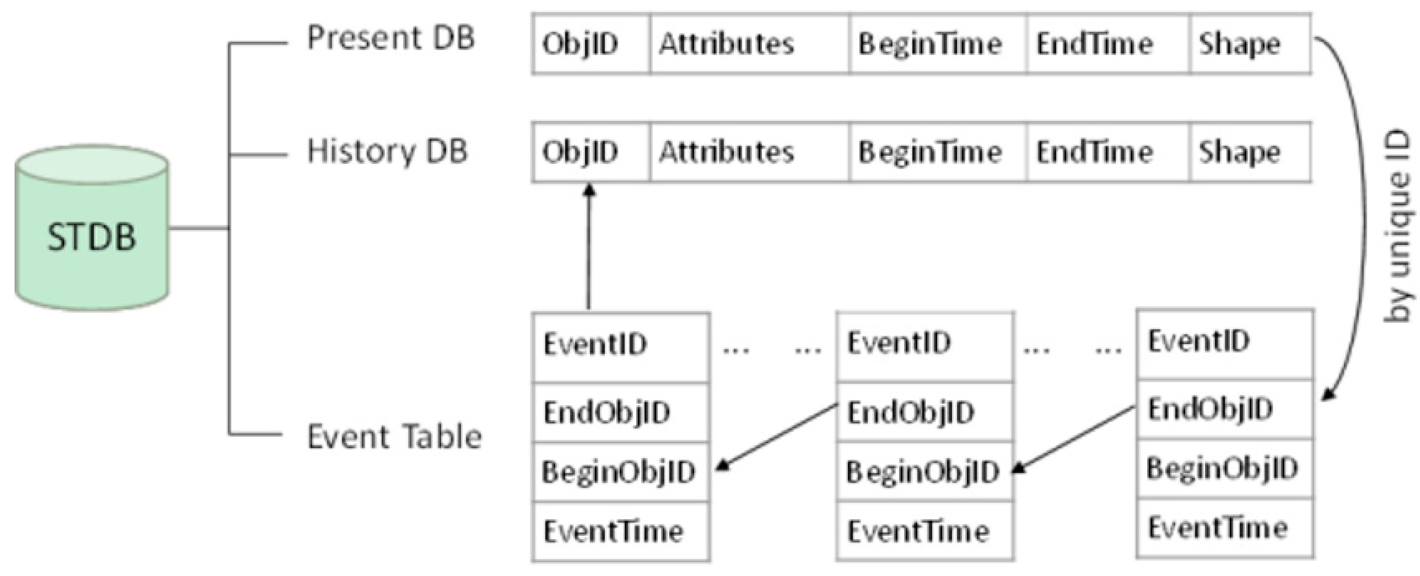
2.2. Statistical Process in STDB
3. Analysis of Land Use Change in Graph Theory Approach
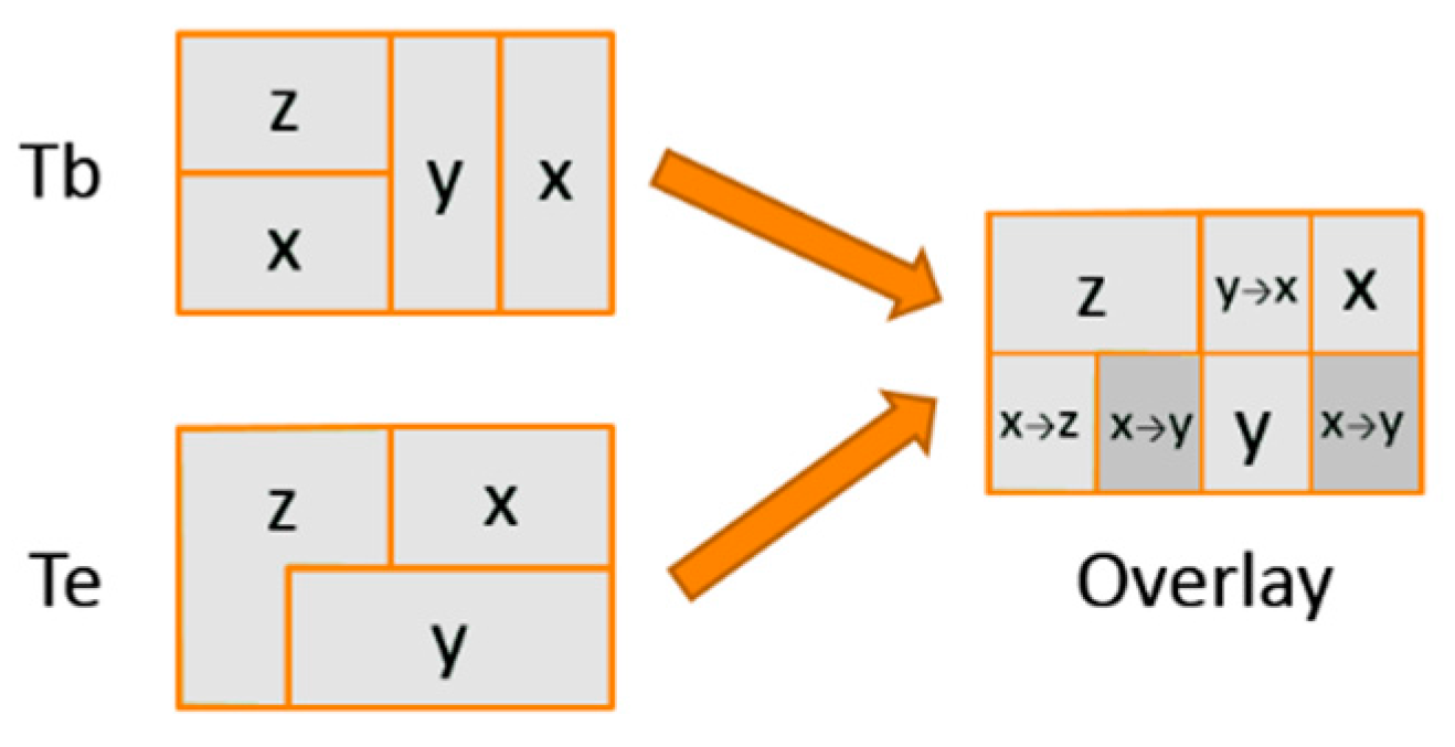
3.1. Characterization of Spatio-Temporal Flow Network
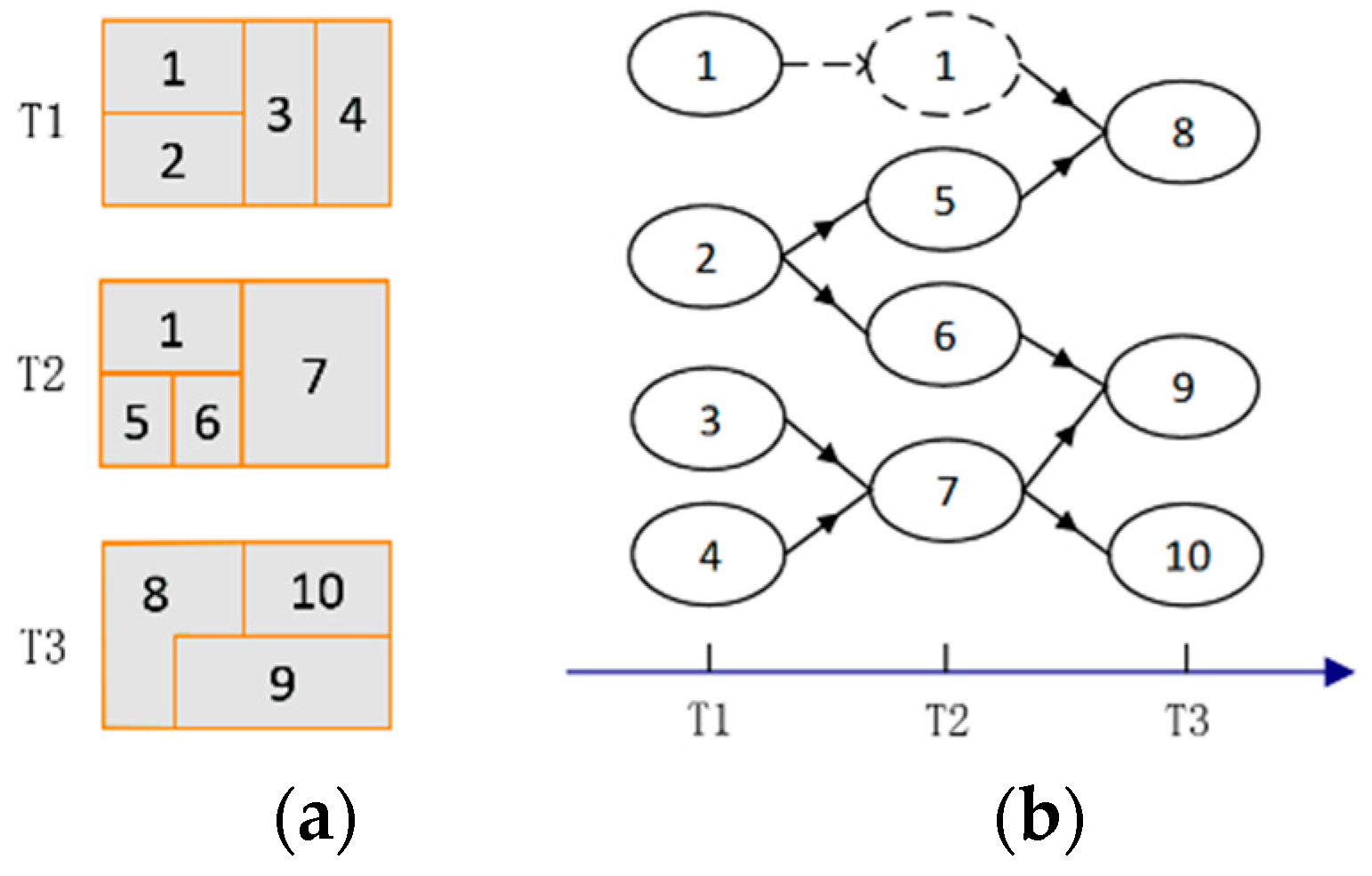

3.2. Modelling Long-Term Transition as Multi-Commodity Flow
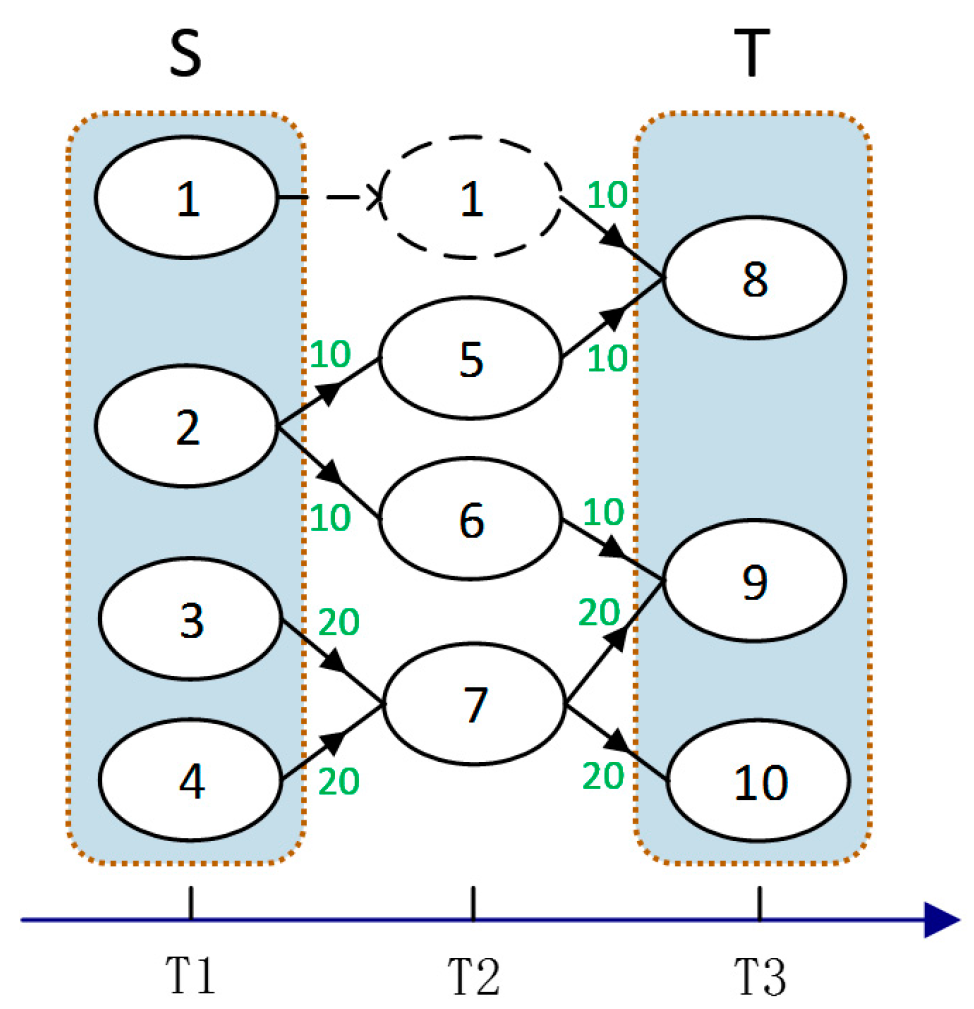
3.3. Constant Multi-Commodity Flow Condition
- , then
- , then v must be reachable from other sources than (otherwise it will be included in ), so it must connect only one sink (or it is a mixed vertex).
- The saturated multi-commodity flow F is constant
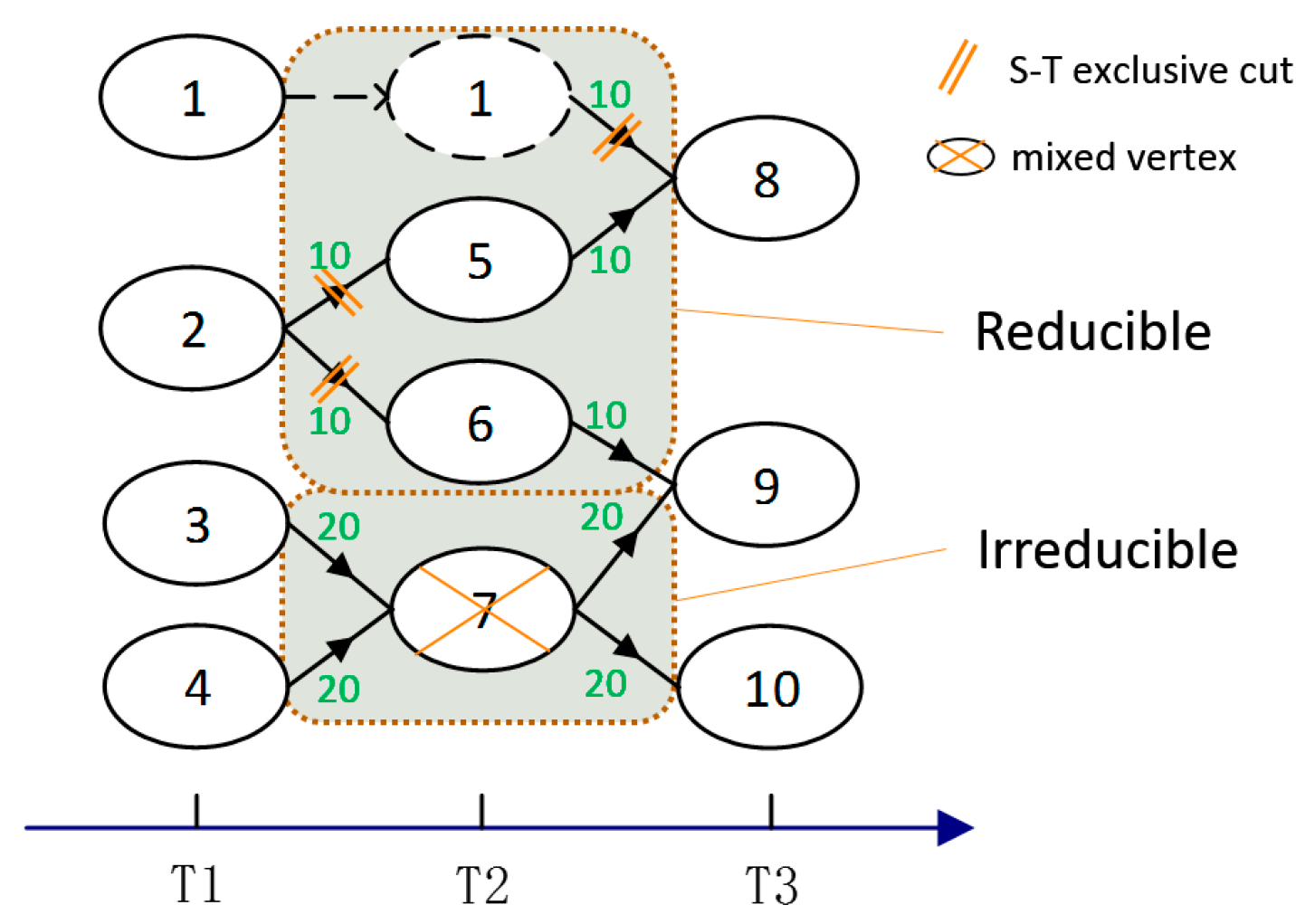
- No mixed vertices exist
- An S-T exclusive cut exists
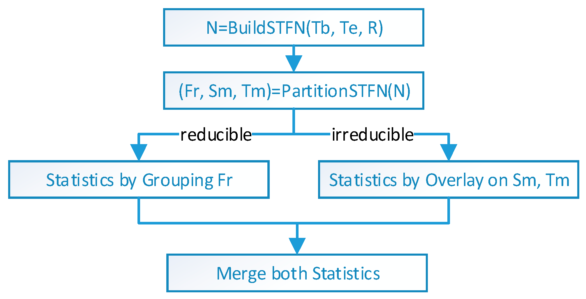
3.4. Reducible or Unreducible
4. Description of the Graph-Based TSP Method
PartitionSTFN(N)
    /* Label T-Reachability */
	Q ← ∅;
	for vertex t ∈ N.T
		 t.Rt ← t;
		 Enqueue t to Q;
    end for
	Begin backward BFS on N using Q;
	while BFS is not complete do
	     Set v to the next vertex in BFS;
         for vertex w in v’s parents
	             w.Rt ← v.Rt ∪ w.Rt;
	     end for
	end while
	/* Label S-Reachability and get decomposition results*/
	Set v.color to white for all vertices in N.V;
	Q ← ∅;
	for each vertex s ∈ N.S
         s.Rs ← s;
	     Enqueue s to Q;
	end for
	Begin forward BFS on N using Q;
	while BFS is not complete do
	     Set v to the next vertex in BFS;
		 if |v.Rs| > 1 and |v.Rt| > 1 then /* mixed vertex */
		        Sm ← Sm ∪ v.Rs;
				Tm ← Tm ∪ v.Rt;
				v.color ← black;
         end if
		 for vertex w in v’s children
		        if v.color = black then
	                   w.color ← black;
	            else if |v.Rs| = 1 and |w.Rt| = 1 then
				       /* find a potential flow in S-T exclusive cut*/
					   Add (s, t, N.c(v,w)) to Fr;
					   w.color ← black;
				end if
				w.Rs ← v.Rs ∪ w.Rs;
		 end for
	end while
	if /* exclude flows from irreducible networks */
	Delete (s, t, c) rows in Fr where s ∈ Sm or t ∈ St;
return Rs, Rt, Fr;
|

5. Data Experiments
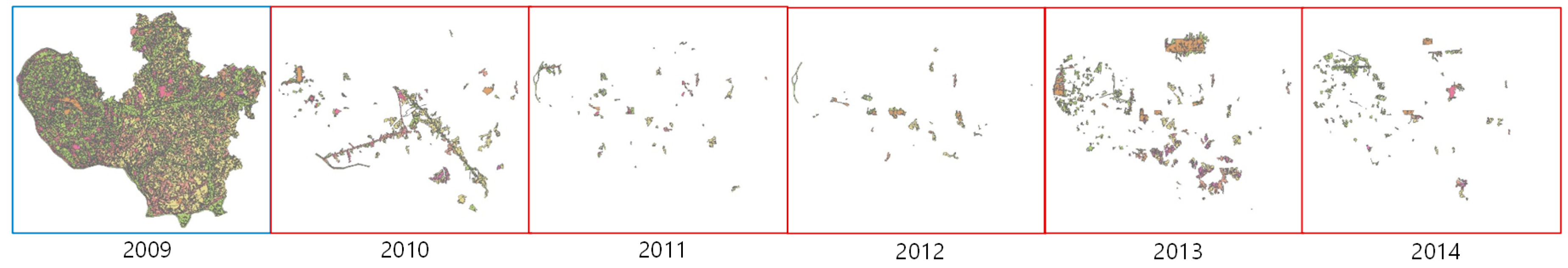
5.1. Sample Data
5.2. Method for Evaluation
5.3. Discussion of the Results

| Query Condition | Basic TSP | Query-Optimized TSP | Graph-Based TSP | |||
|---|---|---|---|---|---|---|
| Amount | Ratio | Amount | Ratio | Amount | Ratio | |
| 2009–2010 | 37,162 | 1.0000 | 2105 | 0.0566 | 0 | 0.0000 |
| 2009–2011 | 37,254 | 1.0000 | 2530 | 0.0679 | 13 | 0.0003 |
| 2009–2012 | 37,311 | 1.0000 | 2613 | 0.0700 | 13 | 0.0003 |
| 2009–2013 | 37,320 | 1.0000 | 3723 | 0.0998 | 20 | 0.0005 |
| 2009–2014 | 38,938 | 1.0000 | 3914 | 0.1005 | 25 | 0.0006 |
6. Conclusions
Acknowledgments
Author Contributions
Conflicts of Interest
References
- Ziadat, F.M.; Taimeh, A.Y. Effect of rainfall intensity, slope and land use and antecedent soil moisture on soil erosion in an arid environment. Land Degrad. Dev. 2013, 24, 582–590. [Google Scholar] [CrossRef]
- De Mûelenaere, S.; Frankl, A.; Haile, M.; Poesen, J.; Deckers, J.; Munro, N.; Veraverbeke, S.; Nyssen, J. Historical landscape photographs for calibration of Landsat land use/cover in the Northern Ethiopian highlands. Land Degrad. Dev. 2014, 4, 319–335. [Google Scholar] [CrossRef]
- Muñoz-Rojas, M.; Jordán, A.; Zavala, L.M.; de la Rosa, D.; Abd-Elmabod, S.K.; Anaya-Romero, M. Impact of land use and land cover changes on organic carbon stocks in mediterranean soils (1956–2007). Land Degrad. Dev. 2015, 26, 168–179. [Google Scholar] [CrossRef]
- Zhao, G.; Mu, X.; Wen, Z.; Wang, F.; Gao, P. Soil erosion, conservation, and eco-environment changes in the loess plateau of China. Land Degrad. Dev. 2013, 24, 499–510. [Google Scholar] [CrossRef]
- Saha, D.; Kukal, S.S. Soil structural stability and water retention characteristics under different land uses of degraded lower himalayas of north-west India. Land Degrad. Dev. 2015, 26, 263–271. [Google Scholar] [CrossRef]
- Keesstra, S.D.; Geissen, V.; van Schaik, L.; Mosse., K.; Piiranen, S. Soil as a filter for groundwater quality. Curr. Opin. Env. Sust. 2012, 4, 507–516. [Google Scholar] [CrossRef]
- Gao, X.; Wu, P.; Zhao, X.; Wang, J.; Shi, Y. Effects of land use on soil moisture variations in a semi-arid catchment: Implications for land and agricultural water management. Land Degrad. Dev. 2014, 25, 163–172. [Google Scholar] [CrossRef]
- Berendse, F.; van Ruijven, J.; Jongejans, E.; Keesstra, S.D. Loss of plant species diversity reduces soil erosion resistance of embankments that are crucial for the safety of human societies in low-lying areas. Ecosystems 2015, 18, 881–888. [Google Scholar] [CrossRef]
- Wang, X.; Bao, Y. Study on the method of land use dynamics change research. Prog. Geogr. 1999, 18, 83–89. [Google Scholar]
- Zhu, H.; Li, X. Discussion on the index method of regional land use change. Acta Geogr. Sinica 2003, 5, 643–650. [Google Scholar]
- Rutherford, G.N.; Bebi, P.; Edwards, P.J.; Zimmermann, N.E. Assessing land-use statistics to model land cover change in a mountainous landscape in the European Alps. Ecol. Model 2008, 212, 460–471. [Google Scholar] [CrossRef]
- Han, H.; Yang, C.; Song, J. Scenario simulation and the prediction of land use and land cover change in Beijing, China. Sustainability 2015, 4, 4260–4279. [Google Scholar] [CrossRef]
- Xie, H.L.; Liu, L.M.; Li, B.; Zhang, X.S. Spatial autocorrelation analysis of multi-scale land-use changes: A case study in Ongniud Banner, Inner Mongolia. Acta. Geo. Sin. 2006, 61, 389–400. [Google Scholar]
- Cormen, T.H.; Leiserson, C.E.; Rivest, R.L.; Stein, C. Computational geometry. In Introduction to Algorithms, 3rd ed.; The MIT Press: Cambridge, MA, USA, 2009; pp. 1022–1027. [Google Scholar]
- Liu, N.; Liu, R.; Zhu, G.; Xie, J. A spatial-temporal system for dynamic cadastral management. J. Environ. Manage. 2006, 78, 373–381. [Google Scholar] [CrossRef] [PubMed]
- Gao, Y.; Pan, Y.; Gao, B.; Zhang, X.; Gao, J.; Zhang, Y. Key Technologies for land use survey oriented spatio-temporal database construction. Sci. Surv. Mapp. 2015, 40, 49–54. [Google Scholar]
- Chen, X.; Wu, H.; Li, X.; Zhang, W. Study on event-based spatio-temporal data model for land use change. J. Imag. Graph. 2003, 8, 957–963. [Google Scholar]
- Teng, L.; Liu, R.; Liu, N. A study on spatio-temporal data model based on feature and event. J. Rem. Sens. 2005, 9, 634–639. [Google Scholar]
- Clementini, E.; Di Felice, P. A comparison of methods for representing topological relationships. Inform. Sci. Appl. 1995, 3, 149–178. [Google Scholar] [CrossRef]
- Tøssebro, E.; Nygård, M. Representing topological relationships for spatiotemporal objects. GeoInformatica 2011, 15, 633–661. [Google Scholar] [CrossRef]
- Tang, Y. The linkage mechanism and incremental extraction of land use updating. Ph.D. Thesis, Zhejiang University, Hangzhou, China, 2011. [Google Scholar]
- Schneider, M. Spatial and spatio-temporal data models and languages. In Encyclopedia of Database Systems; Liu, L., Özsu, M.T., Eds.; Springer US: Medford, MA, USA, 2009; pp. 2681–2685. [Google Scholar]
- Worboys, M.F.; Hearnshaw, H.M.; Maguire, D.J. Object-oriented data modelling for spatial databases. Int. J. Geogr. Inform. Syst. Appl. Rem. Sens. 1990, 4, 369–383. [Google Scholar] [CrossRef]
- Ruan, M.; Liu, R.; Liu, N.; Teng, L. Research on land utilization temporal statistic model based on event. Appl. Resear. Comput. 2005, 7, 31–33. [Google Scholar]
- Wilcox, D.J.; Harwell, M.C.; Orth, R.J. Modeling Dynamic Polygon Objects in Space and Time: A New Graph-based Technique. Cartogr. Geogr. Inform. Sci. 2000, 27, 153–164. [Google Scholar] [CrossRef]
- Yin, Z.; Li, L.; Ai, Z.X. A study of spatio-temporal data model based on graph theory. Acta Geod. Cartogr. Sinica 2003, 32, 168–172. [Google Scholar]
- Spéry, L.; Claramunt, C.; Libourel, T. A spatio-temporal model for the manipulation of lineage metadata. GeoInformatica 2001, 5, 51–70. [Google Scholar] [CrossRef]
- Del Mondo, G.; Rodriguez, M.; Claramunt, C. Modeling consistency of spatio-temporal graphs. Data Knowl. Eng. 2013, 84, 59–80. [Google Scholar] [CrossRef]
- McBride, R. Advances in solving the multicommodity-flow problem. Interfaces 1998, 28, 32–41. [Google Scholar] [CrossRef]
- West, D.B. Introduction to Graph Theory, 1st ed.; Prentice Hall: Upper Saddle River, NJ, USA, 2000; p. 470. [Google Scholar]
- Cormen, T.H.; Leiserson, C.E.; Rivest, R.L.; Stein, C. Linear programming. In Introduction to Algorithms, 3rd ed.; The MIT Press: Cambridge, MA, USA, 2009; pp. 862–863. [Google Scholar]
- Wing, O.; Kim, W.H. The path matrix and switching functions. J. Frankl. Instit. 1959, 268, 251–269. [Google Scholar] [CrossRef]
- Liu, J.; Kuang, W.; Zhang, Z.; Xu, X.; Qin, Y.; Ning, J.; Chi, W. Spatiotemporal characteristics, patterns, and causes of land-use changes in China since the late 1980s. J. Geogr. Sci. 2014, 2, 195–210. [Google Scholar] [CrossRef]
- Žalik, B. Two efficient algorithms for determining intersection points between simple polygons. Comput. Geosci. 2000, 26, 137–151. [Google Scholar] [CrossRef]
- Peuquet, D.J. Time in GIS and Geographical Databases. Geogr. Inform. Syst. 1999, 1, 91–102. [Google Scholar]
- Wang, S.; Zhang, Z.; Zhou, Q.; Wang, C. Study on Spatial temporal features of land use/land cover change based on technologies of RS and GIS. J. Rem. Sens. 2002, 6, 223–228. [Google Scholar]
© 2015 by the authors; licensee MDPI, Basel, Switzerland. This article is an open access article distributed under the terms and conditions of the Creative Commons by Attribution (CC-BY) license (http://creativecommons.org/licenses/by/4.0/).
Share and Cite
Zhang, Y.; Gao, Y.; Gao, B.; Pan, Y.; Yan, M. An Efficient Graph-based Method for Long-term Land-use Change Statistics. Sustainability 2016, 8, 9. https://doi.org/10.3390/su8010009
Zhang Y, Gao Y, Gao B, Pan Y, Yan M. An Efficient Graph-based Method for Long-term Land-use Change Statistics. Sustainability. 2016; 8(1):9. https://doi.org/10.3390/su8010009
Chicago/Turabian StyleZhang, Yipeng, Yunbing Gao, Bingbo Gao, Yuchun Pan, and Mingyang Yan. 2016. "An Efficient Graph-based Method for Long-term Land-use Change Statistics" Sustainability 8, no. 1: 9. https://doi.org/10.3390/su8010009
APA StyleZhang, Y., Gao, Y., Gao, B., Pan, Y., & Yan, M. (2016). An Efficient Graph-based Method for Long-term Land-use Change Statistics. Sustainability, 8(1), 9. https://doi.org/10.3390/su8010009