Sustainable Street Lighting Design Supported by Hypergraph-Based Computational Model

Abstract

Street lighting systems are significant energy consumers in urban environments. The important step toward the reduction of this energy consumption and, thus, finding a balance between functional requirements and savings-related demands, was introducing LED-based light sources. There still exists, however, a margin for further savings, which is associated with well-tailored designs of road lighting installations. The critical impediment that has to be overcame beforehand is the computational complexity related to preparing such a well-suited design. To make this approach feasible, we propose using the formal graph-based model, enabling efficient heuristic computations. In this article, we demonstrate several real-life cases showing a coarse estimation of potential savings in terms of reduced CO${}_2$ emission. The presented results are expressed in kWh of saved energy, metric tones of CO${}_2$, but also as a volume of combusted fuels, to make the assessment more tangible.

1. Introduction

The sustainable development of urban regions is a multidimensional problem covering such fields as access to (limited) resources (e.g., public transport, water, energy), ensuring a balance among different, often “competing” (divergent) objectives of inhabitants, social issues, and so on. Sustainability can be also considered in the broader perspective, i.e., as finding a balance in the scale of a region. In this article, we will stay at the level of an urban environment and focus on the problem related to energy utilization, namely optimizing the performance of public lighting systems. This approach falls into the domain that is sometimes referred to as “smart cities”.

Integral parts of a sustainable development are research and innovation activities. The methods presented in the article are aimed at energy conservation and, as such, can be regarded as an environmental technology. The key issue being critical for their practical applicability, however, is resolving the computational complexity inherent to large-scale projects. This problem is addressed in the paper.

In modern urban environments with populations and populated areas growing dynamically, one faces two opposite factors influencing the development of outdoor lighting systems. The first factor is the necessity of ensuring an appropriate illuminance of public spaces, which is crucial for the public’s safety (in the broad sense) and comfort. The second issue is related economic constraints, which enforce searching for solutions requiring the least financial expenses, in particular corresponding to the energy usage. In this paper, we focus on introducing the approach that supports creating such sustainable solutions. The solutions allow for obtaining high power savings (over 10%) and, on the other hand, do not require the initial investment costs generated by advanced or specialized equipment.

Northeast Group assessed the number of streetlights installed in the world (according to the 2014 report [1]) at over 280 million. This estimation shows the scale of the available energy savings that may be achieved even when assuming a small unit reduction of the power consumption. Those savings are reflected in lower exploitation costs, but also lower emissions of greenhouse gases.

The typical areas of possible energy savings in public lighting are related to applying LED fixtures (the prices of which are continuously falling) and using a range of control methods, such as scheduling or adaptive control. These areas, however, will not be considered here. Another interesting approach intended to reduce the power usage is changing the reflective properties of a road surface rather than replacing high intensity discharge lamps with LEDs. This method, introduced in [2], is applicable especially for road tunnels, where lighting installations work in continuous mode.

In this article, we exploit yet another field of available savings, which is associated with the preparation of a road lighting design. As was proven in [3], we are able to prepare a design (also referred to as the custom design) complying with an existing lighting standard (e.g., [4]), but giving an installation having even 10%–15% lower energy consumption compared to designs made using the industry standard software and the typical standard-based approach [5].

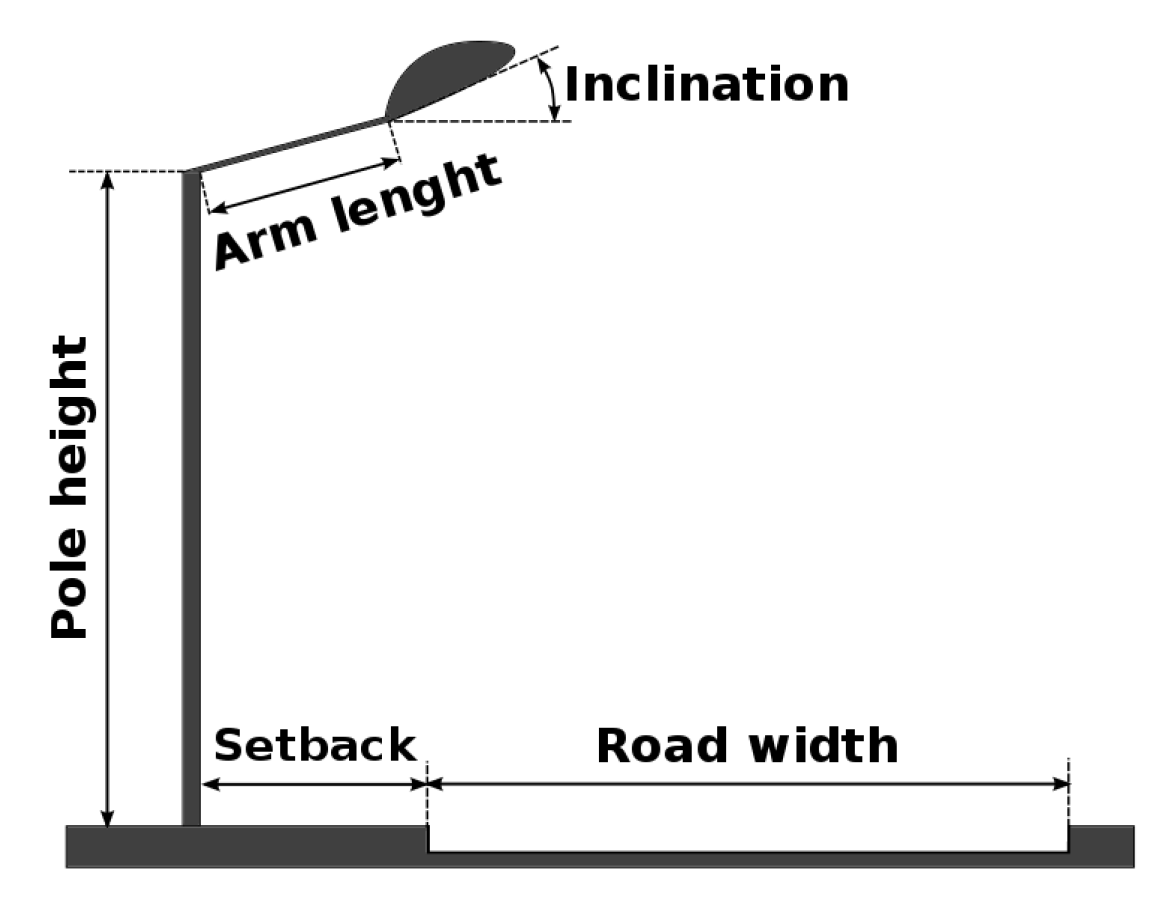
The core concept of the mentioned approach is using actual data (such as luminaire spacings, road width or setback; see Figure 2) rather than the averaged or maximized ones. In particular, it refers to the road geometry and luminaire positions, which are given as high-precision GIS (geographic information system) data. For simple cases of regular layouts containing straight-lined roadways with evenly-distributed luminaires, with no shading objects (like trees), the heuristic methods for designing multi-point installations are known. The problems arise when a lighting situation becomes complex due to the presence of objects or the non-standard geometry of a scene. Such irregularities appear, for example, when one deals with non-evenly-spaced luminaires and a variable road width. Then, the search space gets so large, that the finding a solution becomes not unfeasible in a reasonable amount of time by humans, even when supported by some photometric software, like DIALux [6].

To resolve this problem, two steps have to be taken. The first is describing a design problem in terms of some formal representation comprehensible for a computer program. Such a representation has to be flexible and expressive enough to model a design task, but also it has to enable parallel computations. The second step to be done is the application of the solution-finding heuristic algorithms on the distributed formal model of a given problem. In this phase, the custom design mentioned above is prepared.

Extensive research shows that a graph-based representation fulfills such demands [7,8,9,10,11,12,13,14]. In particular, its expressiveness allows for modeling a range of lighting design problems (including control issues), and on the other side, it may be easily distributed and populated by a multi-agent system performing a solution search [15].

In this paper, we also focus on the computational aspect of a lighting design process, rather than on the photometric one. In particular, the custom calculation approach presented in [3] will not be discussed in detail here. Instead, special focus will be put on graph-based data structures enabling the automated bulk optimization of lighting installations, resulting in the significant reduction of computation time.

The paper is organized as follows. In Section 2, the state of the art is sketched: it contains the description of the lighting design process and the related issues. The hierarchical graph representation of the design is presented in Section 3. The concept of hypergraphs modeling the scene objects is introduced in Section 4. Section 5 contains a description of several real-life cases, and the rough quantitative estimation of the final effects yielded by the proposed approach. In the last section, the final conclusions are given.

2. State of the Art: Outdoor Lighting Design Process

This section gives an overview of a lighting installation design together with its limitations. Next, the problem of the design optimization is discussed. The lighting standards define the calculation methods, but also, the constraints for photometric computations are presented afterwards.

The outdoor lighting design process is carried out according to the rules included in a set of lighting design best practices, e.g., [16,17] and relevant standards [4,5,18]. The important factor influencing a designer’s performance is experience that allows rejecting a priori all solutions that are not compliant with the above rules. Very important help in the design process comes from computer programs, which support three areas: (i) design; (ii) visualization; (iii) quantitative assessment of a solution. Their functionality enables accelerating design steps by using accurate data layers, including a scene layout, localization of luminaires, and so on.

Although the design methodology is mature and equipped with a range of tools [6,19,20], it faces problems related to two areas: optimization, i.e., finding the best solution with respect to the given criteria, and bulk design, which refers to the preparation of designs for multiple (hundreds) of scenes. Both problems may be reduced to the work overhead issue: the number of scenarios to be verified by a designer prevents a human from finding the best solution in a reasonable time, especially when using the trial-and-error approach. On the other hand, the number of potential solutions may be so high that verifying them all using some brute force method is also not doable in the acceptable time. A design task gets proportionally more complicated when considering multiple scenes.

2.1. Design Optimization: Assessment Metrics

The problem of finding an energy-efficient lighting installation is just the case described above. To make it viable, we propose an approach relying on three elements:

• a well-defined, graph-based formalization of a design problem,
• effective algorithms, either exact or heuristic, for finding an optimal solution in a reasonable time,
• a computational method implementing the above algorithms and working with the constraint of an acceptable execution time.

In the sequel, the basic factors influencing solution finding and a solution itself will be presented.

As mentioned above, a design process aims at determining an optimal solution (design). Therefore, some quantitative measure is required for ordering the obtained solutions against a given criterion. There are two scenarios possible. In the fist one, a criterion corresponds to some non-quantitative property, e.g., related to the aesthetics or other subjective characteristics. The ordering by non-quantitative properties may be accomplished using pairwise comparison methods [21], which will not be considered here. In the second case, one deals with measurable parameters. In this article, we focus on the energy efficiency, which is also subject to standardization [22]. For further purposes, however, the custom metrics are defined below.

For a uniform installation I consisting of k rows of luminaires ($R_i,i=1,2,\dots k$), such that:

• luminaire spacing, S, is constant within each row,
• all luminaires from $R_i$ are equipped with the same fixture model,
• all fixtures in $R_i$ work with the same dimming level, d, or, equivalently, with the same luminous flux ratio, $LFR=1-d$,
• the fixture power usage can be expressed with the help of $LFR$: $P=P_0\times LFR$, where $P_0$ is the power consumption of non-dimmed lamp,

the total power may be computed as:

$$\mathcal{P}\left(I\right)=\sum _{R_i}\sum _{f\in R_i}{P}_{0,f}LF{R}_f=\sum _{R_i}{P}_{0,f}LF{R}_f\left|R_i\right|$$

where the outer-most sum iterates over all relevant rows of luminaires; $P_{0,f}$ and $LF{R}_f$ denote a nominal lamp wattage and a luminous flux ratio, respectively, for a fixture f, and $|R_i|$ stands for a number of luminaires in the row $R_i$. In the sequel, we denote $P_{def}=\mathcal{P}\left(I\right)$ (the $def$ subscript stands for default).

For a non-uniform installation $\widehat{I}$, i.e., such that Assumptions 1 and 3 do not need to be satisfied, the total power is given by:

$$\mathcal{P}\left(\widehat{I}\right)=\sum _{R_i}\sum _{f_j\in R_i}{P}_{0,f}LF{R}_{f_j}=\sum _{R_i}\left[P_{0,f}\sum _{f_j\in R_i}LF{R}_{f_j}\right]$$

where $P_{0,f}\equiv P_{0,f_j}$ is a nominal wattage of all fixtures $f_j\in R_i$ and $LF{R}_{f_j}$ is a luminous flux of $f_j$. In the sequel, we denote $P_{cust}=\mathcal{P}\left(\widehat{I}\right)$ (the $cust$ subscript stands for custom).

A uniform installation $I_i$ is said to be better than $I_j$ iff $\mathcal{P}\left(I_i\right)<\mathcal{P}\left(I_j\right)$. Analogously, a non-uniform installation ${\widehat{I}}_i$ is said to be better than ${\widehat{I}}_j$ iff $\mathcal{P}\left({\widehat{I}}_i\right)<\mathcal{P}\left({\widehat{I}}_j\right)$.

The design process is aimed at finding the setup of a given installation (either uniform or non-uniform) yielding the lowest total power value.

2.2. Lighting Standards

Photometric computations being an integral part of a lighting design process are aimed at testing the compliance of a solution against mandatory standards, defining an installation’s performance for different scenarios specified in the standardization [18]. Those scenarios referred to as the lighting situations are defined on the basis of such factors as:

• user type(s) present in an outdoor public traffic area (e.g., pedestrians, slow-moving vehicles),
• typical speed of a main user (e.g., 70 mph, in the case of a highway),
• the type of considered area (e.g., intersection, conflict area),
• traffic flow rate (e.g., 6000 vehicles per day),
• others (e.g., complexity of visual field, ambient brightness level, difficulty of navigational task).

To each lighting situation, an appropriate lighting class is assigned. The standard [4] gives the quantitative description of a lighting installation’s performance for particular classes. For example, Table 1 presents such a specification for so called ME-lighting classes which establish performance requirements for traffic routes of medium to high driving speeds. In this standard, three groups of photometric quantities are considered: (i) luminance of the road surface of the carriageway for the dry road surface condition, which is described by the average road surface luminance ($L_{avg}$), the overall uniformity of the luminance ($U_o$) and the longitudinal uniformity of the luminance ($U_l$); (ii) disability glare, the threshold increment ($TI$); and (iii) the lighting of surroundings, the surround ratio ($SR$). Each lighting design falling into an ME class has to comply with the suitable requirements defined in Table 1.

Table 1. ME- lighting classes according to EN 13201-2.

Class	${\mathbf{L}}_{\mathbf{avg}}\mathbf{(}\mathbf{cd}\mathbf{/}{\mathbf{m}}^{\mathbf{2}}\mathbf{)}$	${\mathbf{U}}_{\mathbf{o}}$	${\mathbf{U}}_{\mathbf{l}}$	$\mathbf{TI}\mathbf{(}\mathsf{\%}\mathbf{)}$	$\mathbf{SR}$
	(min. required)	(min. required)	(min. required)	(max. allowed)	(min. required)
ME1	2.0	0.4	0.7	10	0.5
ME2	1.5	0.4	0.7	10	0.5
ME3a	1.0	0.4	0.7	15	0.5
ME3b	1.0	0.4	0.6	15	0.5
ME3c	1.0	0.4	0.5	15	0.5
ME4a	0.75	0.4	0.6	15	0.5
ME4b	0.75	0.4	0.5	15	0.5
ME5	0.5	0.35	0.4	15	0.5
ME6	0.3	0.35	0.4	15	n/a

Table 1. ME- lighting classes according to EN 13201-2.

Class	${\mathbf{L}}_{\mathbf{avg}}\mathbf{(}\mathbf{cd}\mathbf{/}{\mathbf{m}}^{\mathbf{2}}\mathbf{)}$	${\mathbf{U}}_{\mathbf{o}}$	${\mathbf{U}}_{\mathbf{l}}$	$\mathbf{TI}\mathbf{(}\mathsf{\%}\mathbf{)}$	$\mathbf{SR}$
	(min. required)	(min. required)	(min. required)	(max. allowed)	(min. required)
ME1	2.0	0.4	0.7	10	0.5
ME2	1.5	0.4	0.7	10	0.5
ME3a	1.0	0.4	0.7	15	0.5
ME3b	1.0	0.4	0.6	15	0.5
ME3c	1.0	0.4	0.5	15	0.5
ME4a	0.75	0.4	0.6	15	0.5
ME4b	0.75	0.4	0.5	15	0.5
ME5	0.5	0.35	0.4	15	0.5
ME6	0.3	0.35	0.4	15	n/a

2.3. Scene Layouts

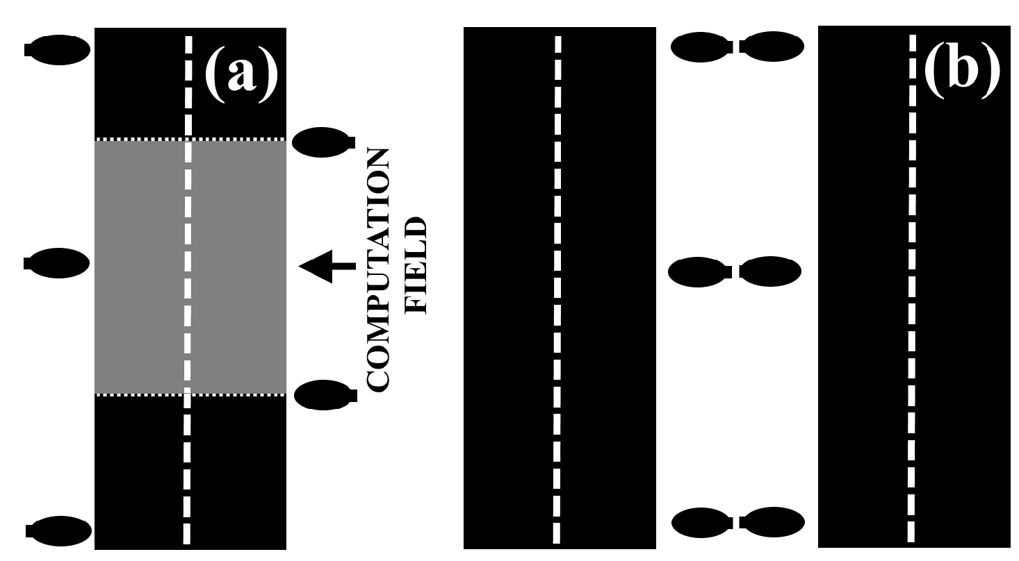
In this article, we focus especially on roadway layouts. Two major types of roads can be considered here: single and double carriageways. To each of them, luminaires arranged in some order are ascribed (Figure 1). Such a layout is subject to a design process.

Since the geometric properties of a layout are not ideal, i.e., the subsequent luminaire spacings or post setbacks are not uniform, one can carry out the design process in two manners. In the first approach, the aggregated values are used instead of actual ones (Figure 2). In this case, the aggregates (usually the maxima) reflect a pessimistic scenario in which a computation field has the largest possible size. This assumption guarantees obtaining a standard compliant solution, but yields, as the side-effect, an unwanted over-illumination. Another, alternative approach, is using the actual layout data and performing computations field-by-field. This approach gives the perfectly-tailored lighting design in terms of the illumination level and energy usage.

Figure 1. Luminaire arrangement examples: (a) staggered left; (b) twin.

Figure 1. Luminaire arrangement examples: (a) staggered left; (b) twin.

Figure 2. The adjustable parameters of the luminaire.

Figure 2. The adjustable parameters of the luminaire.

The cost paid for the high quality of a solution is the significant workload related to the design and corresponding photometric computations. To resolve this issue, we propose applying in parallel the heuristic algorithms reducing the time of solution finding. The important step, however, prior to the parallel processing is formalizing a design problem in such the way that using those heuristics is feasible. This formalization has to have a sufficient expression power for modeling a scene, and on the other hand, it has to support the processing parallelization.

The hierarchical graph-based representation introduced in Section 3 satisfies those requirements. Additionally, it enables applying a multi-agent system in the phase of parallel processing.

2.4. Design Process Complexity

To substantiate using a graph-based representation of a scene in photometric calculations, it is enough to make a rough estimation of the design process complexity. We focus on its default version, i.e., when the spacing, road width, setback, and so on, are uniform for the entire installation/road layout (see Figure 2). It is assumed that for obtaining the optimal solution (in terms of the energy usage), one can vary the parameters shown in Table 2.

Table 2. Variable parameters of the design process.

Parameter	Range	Step	Number of Variants
Pole height	6–10 m	0.5 m	9
Arm length	0.5–3 m	0.5 m	6
Fixture inclination	5${}^{°}$–20${}^{°}$	5${}^{°}$	4
Fixture dimming level	$0\mathsf{\%}–75\mathsf{\%}$	$1\mathsf{\%}$	76
Fixture model	n/a	n/a	500

Table 2. Variable parameters of the design process.

Parameter	Range	Step	Number of Variants
Pole height	6–10 m	0.5 m	9
Arm length	0.5–3 m	0.5 m	6
Fixture inclination	5${}^{°}$–20${}^{°}$	5${}^{°}$	4
Fixture dimming level	$0\mathsf{\%}–75\mathsf{\%}$	$1\mathsf{\%}$	76
Fixture model	n/a	n/a	500

The total number of variants to be checked, N, is the product:

$$N=9\times 6\times 4\times 76\times 500=8,208,000.$$

Even assuming that expert knowledge enables a designer to reject some variants, say half, without detailed analysis, a number of the remaining ones will be still too large to process with the participation of a human. In such a case, a designer would be a bottleneck for the process. In the next section, the graph-based formalization of a design problem will be presented. This allows for applying a fully-automated and time-efficient method for solution finding.

3. Hierarchical Graph Representation

In this section, the hierarchical, two-level representation of a scene will be presented. The general concept of this representation is considering a scene at two levels: a level of a low and of a high granularity, respectively. For the former level, a scene is modeled with the help of an undirected, labeled and attributed graph (Definition 1). Objects and spaces are represented as the graph’s nodes and the spatial and logical relationships among them as the edges. Objects refer to any entities, including the buildings, areas (lawns, roads, squares, junctions and other functionally-defined ones), street fixtures or lighting infrastructure components (luminaires, control cabinets, sensors, and so on). Each node encapsulates all design-required information, necessary to perform photometric computations.

To get those data, one enters the lower and high granularity level of the model. At this level, the relevant graph nodes are transformed into hypergraphs defined below (Definition 3), representing subsequent objects. The graph edges from the upper level are inherited to the lower one.

The important property of the graph representation is that it may be easily distributed [23,24] (see Definition 2). Thanks to this, we are able to make the transition from the lower level to its distributed form using the concept of a slashed hypergraph (Definition 5) and to get an environment ready for a multi-agent system deployment.

The concept of the slashed form of a centralized graph G allows for distributing G in such a way that the coupling among resultant subgraphs, in terms of shared elements, is minimal. Thanks to this, the distributed processing performed by a multi-agent system is not throttled by a communication overhead.

The formal definitions of the structures being used are presented below.

Definition 1 

($\Sigma A$-graph). $\Sigma A$-graph is a triple $G=(V,E,\phi )$, where V is a non-empty set of nodes, $E\subseteq V\times ({\Sigma }^e\times A)\times V$ is a set of directed edges, $\phi :V⟶{\Sigma }^v$ is an attributing function, ${\Sigma }^v$ and ${\Sigma }^e$ denote sets of node and edge labels, respectively, and A is a set of edge attributes. We denote the family of $\Sigma A$-graphs as $\mathcal{G}$.

The edge structure is the cross product $V\times ({\Sigma }^e\times A)\times V$ to enable storing all data required in the design process in edge attributes. In particular, these data can include such problem-specific information as architectural details of adjacent buildings. The $\Sigma A$-graph definition can be also extended by introducing an attributing function for nodes, but such an extension does not impact further considerations, so it will not be considered here.

Definition 2 

(Slashed form of G). Let $G=(V,E,\phi )\in \mathcal{G}$. A set $\left\{G_i\right\}$ of graphs is defined as follows.

• $G_i=(V_i,E_i,{\phi }_i)\in \mathcal{G}$ and $V_i=C_i\cup D_i,C_i\cap D_i=\varnothing$, where $C_i$ is a set of core nodes, $D_i$ denotes a set of dummy nodes and ${\phi }_i{\equiv \phi |}_{V_i}$ (a restriction of φ mapping to $V_i$ set),
• ${\bigcup }_i{C}_i=V$ where $C_i,C_j$ are mutually disjoint for $i\ne j$,
• $\forall v\in D_i\exists !v^{\prime }\in D_j(i\ne j)$, such that $v^{\prime }$ is the replica of v; $\forall v\in D_{i}deg\left(v\right)=1$,
• $\forall e\in E_i:e$ is incident to at last one dummy node.

An edge incident to a dummy node is called a border edge. The set of all border edges in $G_i$ is denoted as $E_i^b$. The set $E_i^c=E_i-E_i^b$ is referred to as a set of core edges of $G_i$. Let $M={\Sigma }^e\times A$; then, a set $\left\{G_i\right\}$ as defined above is referred to as a slashed form of G and denoted , iff the following conditions are satisfied:

• $\forall G_i^c=(C_i,E_i^c,{\phi }_i{|}_{C_i})\exists H_i\subset G:H_i\stackrel{\alpha }{\simeq }{G}_i^c$ (α denotes an isomorphic mapping between graphs) and $H_i,H_j$ are disjoint for $i\ne j$.
• $\exists f:M^2\to M$, a bijective mapping $\forall (e,e^{\prime })\in E_i^b\times E_j^b(i\ne j)$, such that (i) $e=(x_c,m,v)\in C_i\times M\times D_i,e^{\prime }=(v^{\prime },m^{\prime },y_c)\in D_j\times M\times C_j$ and (ii) $v^{\prime }$ is a replica of $v:\exists !e_{ij}=(x,m_e,y)\in E\mathrm{such} \mathrm{that} x_c=\alpha \left(x\right),y_c=\alpha \left(y\right)$ and $f(m,m^{\prime })=m_e$. $e_{ij}$ is called a slashed edge associated with replicated dummy nodes $v,v^{\prime }$.
• $\forall e=(x,m,y)\in E:$ (i)$\exists !e_c\in E_i^c$ for some i, such that $e_c=\alpha \left(e\right)$ or (ii) $\exists !(v,v^{\prime })\in D_i\times D_j$ for some $i,j$, such that e is a slashed edge associated with v and $v^{\prime }$.

$G_i\in$ is called a slashed component of G.

Note that f mapping recovers the attributing data of a slashed edge based on the attribution of given border edges.

Remark:

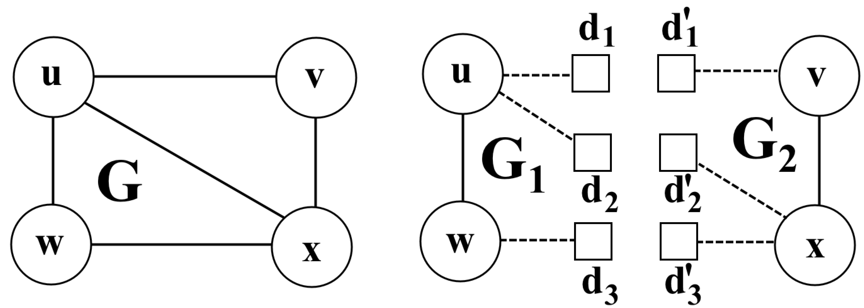
To preserve the clarity of images, we neglect the attributing of graph edges in figures. Figure 3 presents the example of a centralized graph and its slashed form.

Figure 3. The centralized graph, G (left); and its slashed form; $=\{G_1,G_2\}$ (right). Dummy nodes are plotted as squares and border edges as dashed lines.

Figure 3. The centralized graph, G (left); and its slashed form; $=\{G_1,G_2\}$ (right). Dummy nodes are plotted as squares and border edges as dashed lines.

As shown in [25], applying the slashed graphs formalism supported by supplementary heuristics (the so-called reuse method) allows obtaining significant acceleration of photometric computations, which are essential for a street lighting design. The tests made for the centralized graph $G=(V,E)$ modeling an urban space, such that $\left|V\right|=1500$ and $\left|E\right|=2886$, demonstrated that the computation time is reduced by 26.5, from 3250.2 s for a centralized graph to 122.7 s for its slashed form.

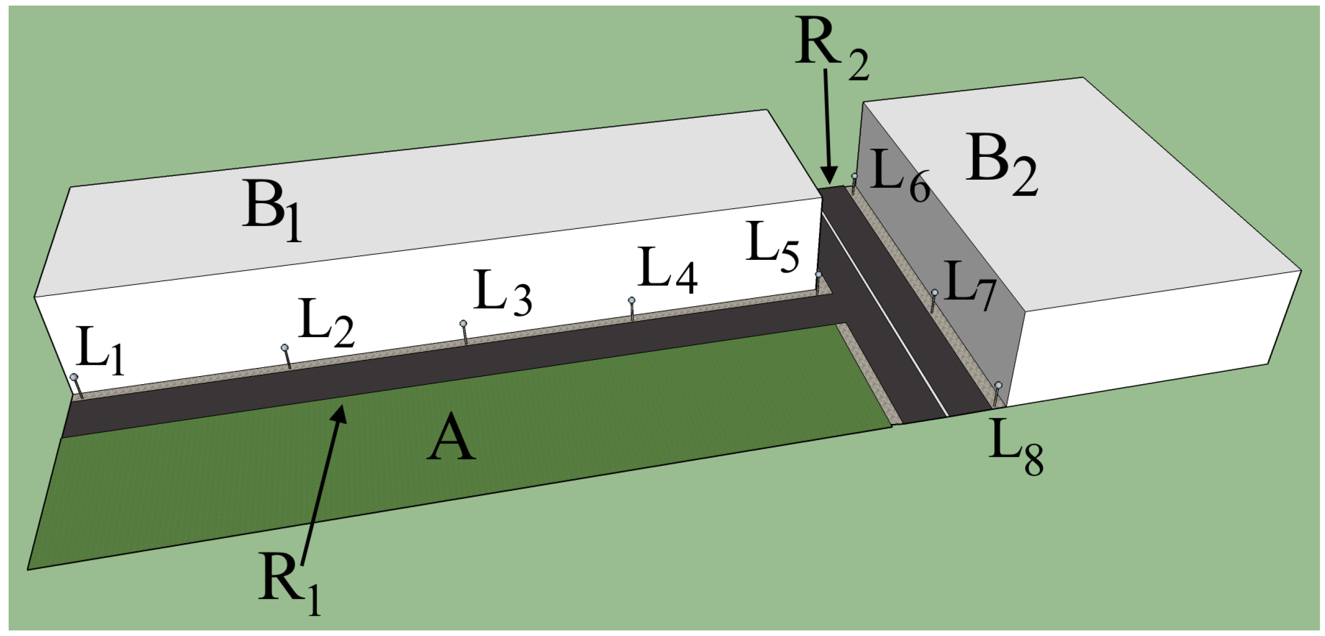
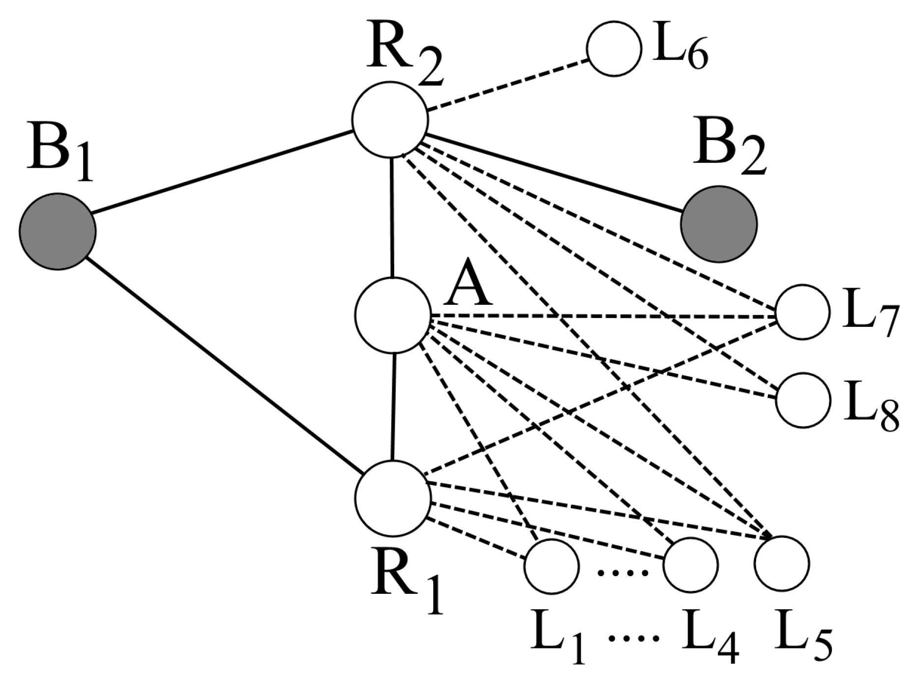
In Figure 4, the simplified scene is shown. It consists of the single and two-lane carriageways ($R_1,R_2$, respectively) with sidewalks alongside, two buildings ($B_1,B_2$), the recreation area (lawn, A) and street luminaires ($L_1,\dots L_8$). The upper (low granularity) level graph representation of this scene is shown in Figure 5. The white nodes (i.e., all except $B_1$ and $B_2$), which represent luminaires and areas (surfaces), are inherited to the lower level as is. The edges incident with $L_i$ nodes (marked with dashed lines) represent the relation of illuminating a surface by a luminaire. In particular, a single luminaire may illuminate several different roads (areas).

Figure 4. The sample scene: $R_1$, single-lane carriageway with sidewalk; $R_2$, two-lane carriageway with two sidewalks alongside; $B_1,B_2$, buildings; A, lawn; $L_1,\dots L_8$, luminaires.

Figure 4. The sample scene: $R_1$, single-lane carriageway with sidewalk; $R_2$, two-lane carriageway with two sidewalks alongside; $B_1,B_2$, buildings; A, lawn; $L_1,\dots L_8$, luminaires.

Figure 5. The upper level graph representation of the scene shown in Figure 4.

Figure 5. The upper level graph representation of the scene shown in Figure 4.

4. Hypergraph Representation

For a given solid consisting of faces, physical edges and physical vertices (contrary to graph edges and graph vertices), the hypergraph representation is introduced. The correspondence among solid features and hypergraph components is as follows: solid faces are represented by hypergraph nodes, solid edges by hypergraph regular edges (i.e., edges connecting two nodes only) and solid vertices by hyperedges. 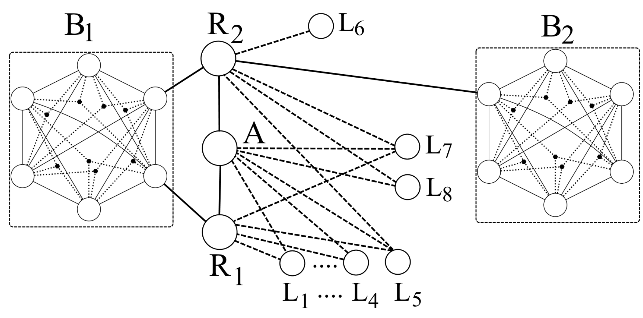Figure 6 shows the hypergraph containing two sub-hypergraphs modeling buildings (cuboids) $B_1$ and $B_2$ belonging to the considered scene.

The formal definition of a hypergraph is given below.

Definition 3 

(Hypergraph). A hypergraph $G_S$ of an object S is a tuple of the form:

$$G_S=(N,A,H,{\left\{la{b}_{\mu }\right\}}_{\mu =N,A,H},{\left\{at{t}_{\mu }\right\}}_{\mu =N,A,H})$$

where N is a nonempty set of nodes, $A\subset P_2\left(N\right)$ is a nonempty set of edges, $H\subset {\bigcup }_{i>2}{P}_i\left(N\right)$ is a nonempty set of hyperedges, $la{b}_{\mu }:\mu \to {\mathcal{L}}_{\mu }$ for $\mu =N,A,H$ is a labeling function for vertices, edges and hyperedges, respectively, with corresponding set of labels ${\mathcal{L}}_{\mu }$, and $at{t}_{\mu }:\mu \to {\mathcal{A}}_{\mu }$ for $\mu =N,A,H$ is an attributing function for vertices, edges and hyperedges, respectively, with corresponding set of attributes ${\mathcal{A}}_{\mu }$.

Figure 6. The lower level graph representation of the scene shown in Figure 4. Bounding boxes $B_1$ and $B_2$ delimit hypergraphs encapsulated inside the upper level nodes, $B_1$ and $B_2$, respectively.

Figure 6. The lower level graph representation of the scene shown in Figure 4. Bounding boxes $B_1$ and $B_2$ delimit hypergraphs encapsulated inside the upper level nodes, $B_1$ and $B_2$, respectively.

The detailed description of the formalism underlying the hypergraph-based model of solids may be found in [26]. It should be remarked that this formalism is flexible and expressive enough to represent nontrivial manifolds. Thanks to the attributing functions, which can store advanced geometric features of objects, a sphere or a cylinder can be modeled as hypergraphs.

Definition 4 

(Composed hypergraph). A composed hypergraph G over the finite set of hypergraphs $G_{S_1},\dots G_{S_k}$ defined above is a tuple of the form:

$$G=({\left\{G_{S_i}\right\}}_{i=1,2,\dots k},E)$$

where E is the finite set of so-called external edges of the form $e=\{u\in N\left(G_{S_i}\right),w\in N\left(G_{S_j}\right)\}\text{for}i\ne j$.

Definition 5 

(Slashed hypergraph). Let G be a composed hypergraph $G=({\left\{G_{S_i}\right\}}_{i=1,2,\dots k},E)$. Then, we define a $\Sigma A-$graph (see Definition 1):

$$G_F=(V,E,\phi )$$

where $V={\left\{G_{S_i}\right\}}_{i=1,2,\dots k}$ is a finite set of nodes corresponding to particular hypergraphs and φ is some node attributing function. The slashed form of the hypergraph G over the set $G_{S_1},G_{S_2},\dots G_{S_k}$ is the slashed form of $G_F$, i.e., . is also referred to as a slashed hypergraph G.

Figure 6 shows the composed hypergraph G representing the considered scene. As was remarked previously, some of its nodes are inherited from the upper-level representation without any changes ($A,R,L$). Furthermore, the edges incident to those nodes are present at this level. The only difference is that the endpoints of edges connecting encapsulating nodes (e.g., $B_1$) change their endpoints. As shown in Figure 6, the edges connecting previously $R_1$ and $R_2$ with $B_1$ are attached now to two different nodes (representing faces of $B_1$ adjacent to the roads $R_1$ and $R_2$) of a relevant hypergraph.

Such low-level, hypergraph representation after decomposition based on the slashed hypergraph concept is ready for a multi-agent system deployment: each agent is hosted by a single slashed component. Thus, parallel processing may be performed to solve a number of lighting design tasks.

5. Case Study

The presented formalism was used in the ISE (the Polish acronym of the name: Intelligent Power Networks) Project [27], which was aimed at the modernization of a part of the existing road lighting infrastructure in the city of Cracow, Poland. The primary goal was replacing almost 3800 high-intensity discharge (sodium vapor) lamps located along 239 streets with LED fixtures. The areas of particular streets were subdivided into 601 uniform calculation segments for which the lighting installation optimization was performed.

5.1. Formalization: Building the Model

A low granularity graph representation (an upper level of the graph hierarchy) of the system being optimized modeled three types of physical/logical objects, namely: calculation segments, luminaires and sensors (involved in control tasks; not considered here). The following relations created associations among the above entities:

• neighborhood (segment-segment),
• impact on an illuminance level (luminaire-segment),
• membership of a detection area (sensor-segment).

$\Sigma A$-graph $G=(V,E,\phi )$, modeling the system consisted of the set of nodes, V, representing entities, the set of edges, E, representing relations and $\phi :V⟶A_V$ being a mapping, attributing graph nodes.

A high granularity system description (a lower level of the graph hierarchy), in turn, relied on the concept of composed hypergraphs (see Definition 4) representing the buildings.

Taking into account such a structure of the scene, we obtained a total number of optimization tasks equal to 2087. This number resulted from the decomposition of the centralized graph of the system into multiple subgraphs processed in parallel. The optimization performed on the four core CPU (Intel CORE i7) took 4 hours 47 minutes compared to 13 hours 12 minutes in the non-parallelized, centralized approach case. This ratio increases significantly when computing using multiple multi-core boxes. This aspect, however, will not be discussed here.

5.2. Environmental Impact

In this section, we analyze three roadways (denoted as Roadways A, B and C, respectively) selected from the hose considered in the ISE Project. The goal of the analysis is investigating the benefits (in terms of the energy usage and the reduced CO${}_2$ emission) obtained thanks to using the custom design method instead of the default one.

Two measures, normalized with respect to the installation length, will be applied to this assessment: the absolute power savings for a given installation (Equation (1)) and the annual volume of the reduced CO${}_2$ emission (Equation (2)) corresponding to this power:

$$\begin{array}{cc}\hfill \Delta P& =P_{cust}-P_{def}\hfill \end{array}$$

(1)

$$\begin{array}{cc}\hfill M_{{\mathrm{CO}}_2}& =F[\Delta P·t_{on}]\hfill \end{array}$$

(2)

where $t_{on}$ refers to the annual lighting time and F is the function converting energy to the CO${}_2$ emission volume (computations are made using the calculator available on the Environmental Protection Agency web site [28]). $\Delta P$ denotes the power savings achieved thanks to using the custom design approach [3]. The reference value ($P_{def}$) is the power of an installation designed using the default, standard-based method.

We assume that no street lighting control is used (e.g., scheduling). Then, the $t_{on}=4285\mathrm{h}$ for the city of Cracow.

It is also assumed that for each single luminaire, the following properties are given (see Figure 2):

• high accuracy ($1\mathrm{cm}$) GPS coordinates of the pole,
• setback,
• corresponding road width,
• spacing to the next luminaire.

Moreover, the following properties common for all luminaires (for a given case) are known: pole height, arm length, fixture model and settings (e.g., dimming, inclination angle). Table 3 presents the summary data describing Roadways A, B and C.

Using the straightforward calculations (after earlier preparation of the custom design), it may be easily found that for 1000 m-long sections of the considered roadways, the total annual energy saved thanks to using the custom lighting design method ($\Delta E=\Delta P\times t_{on}$) and the corresponding volume of the reduced CO${}_2$ emission, $M_{{\mathrm{CO}}_2}$, are 4612.7 kWh/year and 3.184 MT/year, respectively. This amount is equivalent to the volume of CO${}_2$ produced by combustion of 1343.82 liters of gasoline or 1538.59 kilograms of coal. The breakdown by particular roadway is shown in Table 4.

Table 3. Properties of the tested roadways.

Roadway →	A	B	C
Number of luminaires	30	20	8
Luminaire arrangement	single sided
Fixture	BGP353 T45 1xECO163-2S_830 DW	BGP353 T45 1xECO104-2S_830 DW	BGP353 T35 1xECO174-2S_830 DW
Nominal fixture wattage (W)	164.1	110.7	177.4
Lighting class	ME5	ME4a	ME3a
Number of lanes	2	2	1
Luminaire spacing (m)
Min	26.44	25.13	20.24
Max	33.18	35.61	28.23
Avg	29.15	27.20	24.66
Road width (m)
Min	7.67	6.81	7.27
Max	9.16	8.45	8.67
Avg	7.81	7.44	8.28

Table 3. Properties of the tested roadways.

Roadway →	A	B	C
Number of luminaires	30	20	8
Luminaire arrangement	single sided
Fixture	BGP353 T45 1xECO163-2S_830 DW	BGP353 T45 1xECO104-2S_830 DW	BGP353 T35 1xECO174-2S_830 DW
Nominal fixture wattage (W)	164.1	110.7	177.4
Lighting class	ME5	ME4a	ME3a
Number of lanes	2	2	1
Luminaire spacing (m)
Min	26.44	25.13	20.24
Max	33.18	35.61	28.23
Avg	29.15	27.20	24.66
Road width (m)
Min	7.67	6.81	7.27
Max	9.16	8.45	8.67
Avg	7.81	7.44	8.28

Table 4. Power savings and ${\mathrm{CO}}_2$ reduction obtained thanks to the custom computational method (both normalized to 1000 meters of a lighting installation).

Roadway	$\Delta \mathbf{E}(\mathbf{kWh}/\mathbf{year})$	$M_{{\mathrm{CO}}_2}(MT/year)$	Equiv.Amount of Gasoline Consumed (L)	Equiv. Amount of Coal Combusted (kg)
A	1141.99	0.765	325.92	372.85
B	3090.15	2.100	882.00	1010.60
C	473.83	0.319	135.90	155.13
Total	4612.7	3.184	1343.82	1538.59

Table 4. Power savings and ${\mathrm{CO}}_2$ reduction obtained thanks to the custom computational method (both normalized to 1000 meters of a lighting installation).

Roadway	$\Delta \mathbf{E}(\mathbf{kWh}/\mathbf{year})$	$M_{{\mathrm{CO}}_2}(MT/year)$	Equiv.Amount of Gasoline Consumed (L)	Equiv. Amount of Coal Combusted (kg)
A	1141.99	0.765	325.92	372.85
B	3090.15	2.100	882.00	1010.60
C	473.83	0.319	135.90	155.13
Total	4612.7	3.184	1343.82	1538.59

Contrary to the industry standard computing scheme, the photometric calculations were performed individually for all subsequent calculating fields. The power reduction (in relation to the default design method) achieved thanks to applying this approach varied between 10% and 14% depending on the scene being considered.

The above results prove that the suggested area of available energy savings has a significant potential. In turn, the proposed computational approach, based on the concept of slashed hypergraphs, enables performing underlying lighting design tasks effectively, which is crucial for their practical feasibility. This is possible thanks to parallelization and applying heuristic algorithms.

6. Conclusions

In this article, we focused on the unexploited area of available energy savings in an urban environment. This area is related to the preparation of the well-suited lighting designs, which yield lighting installations operating at the power consumption level guaranteeing conformance with mandatory standards for public lighting and, on the other side, eliminating over-illumination, being a symptom of energy wasting.

Since making such an energy-saving lighting design is not feasible in a reasonable amount of time using industry standard tools, we proposed a computational method that can handle the preparation of such designs at the scale of multiple streets, even an entire city. This method relies on a hierarchical hypergraph model of a scene, which enables the distribution of a design task and performing those computations in parallel. This step together with using the special heuristic methods (not discussed here) are crucial for achieving the acceptable time complexity of a design operation.

The proposed approach was applied practically within the ISE project sponsored by the National Fund for Environmental Protection and Water Management (Poland). The results obtained for this real-life case showed that this method has a significant impact on roadway lighting energy cost reduction and, on the other side, on reducing emissions of CO${}_2$. It should be emphasized that the approach does not require implementing any additional, possibly high-cost technologies.

The presented case study describing real-life situations enables formulating the following conclusions.

• The custom design method, which is proven to bring significant power savings, can be applied to large optimization problems, like city-scale retrofits. It is possible thanks to defining a suitable formal representation of a lighting design problem and applying a computational framework relying on multi-agent systems.
• Savings may be achieved for all road types and lighting classes, including bike lanes, walkways, and so forth.
• The proposed method does not require any additional costs related to the supplementary equipment, like sensors network infrastructure (required for control).
• The falling prices of LED sources make the proposed approach very promising and competitive with the “classic” design paradigm.