
Phenological Changes of Corn and Soybeans over U.S. by Bayesian Change-Point Model

Abstract
:
1. Introduction
2. Methodology
2.1. Study Areas and Datasets

| Corn | planted | NC (1981, 1982, 1985, 1995) |
| silking | NC (1981–1983, 1985, 1991, 1994, 1995, 2002, 2004, 2010, 2011, 2013), CO (1981), IN (1981), MI (1981), OH (1981), PA (1981), SD (1981), WI (1981) | |
| mature | NC (1981–1986, 1990–2002, 2004, 2006, 2008–2011, 2013), KY (1995), KS (1991), MO (1983, 1991), PA (1984, 1988, 1991) | |
| Soybean | planted | LA (2001, 2011), MS (2001, 2004–2006, 2010), MN (1998) |
| blooming | LA (2001, 2006, 2009–2011, 2013), MS (1996, 2001, 2003–2011, 2013) | |
| dropping leaves | LA (2013), MS (2004–2006), NC (1981, 1987, 1992), AR (1992) |
2.2. Bayesian Change-Point Model
2.3. Bayesian Model Selection
2.4. Change-Point Parameter Estimation
3. Results


| No | State | Planted | Silking | Mature | Vegetative | Reproductive | Growing Season | ||||||
|---|---|---|---|---|---|---|---|---|---|---|---|---|---|
| s | r | s | r | s | r | s | r | s | r | s | r | ||
| 1 | CO | 0.06 | 4.1 | −0.19 * | 4.0 | −0.12 | 4.9 | −0.25 * | 4.3 | 0.08 | 3.3 | −0.18 | 5.6 |
| 2 | IL | −0.19 | 8.9 | −0.14 | 6.7 | 0 | 9.0 | 0.05 | 6.0 | 0.13 | 6.5 | 0.18 | 8.6 |
| 3 | IN | −0.24 | 9.6 | −0.23 | 6.6 | 0.13 | 8.3 | 0.01 | 6.8 | 0.36 * | 4.2 | 0.37 * | 8.3 |
| 4 | IA | −0.25 * | 6.1 | −0.12 | 5.6 | −0.03 | 8.1 | 0.12 | 5.0 | 0.09 | 4.5 | 0.21 | 7.6 |
| 5 | KS | −0.19 | 6.7 | −0.42 * | 5.3 | −0.23 | 7.5 | −0.22 * | 4.2 | 0.18 | 6.0 | −0.04 | 6.7 |
| 6 | KY | −0.42 * | 10.9 | −0.31 * | 7.4 | −0.47 * | 8.9 | 0.11 | 6.5 | −0.16 | 7.8 | −0.05 | 11.2 |
| 7 | MI | −0.14 | 5.9 | −0.2 | 5.6 | −0.01 | 9.5 | −0.06 | 5.1 | 0.19 | 5.9 | 0.13 | 9.4 |
| 8 | MN | −0.32 * | 6.9 | −0.26 * | 6.0 | 0.03 | 9.2 | 0.06 | 5.4 | 0.29 * | 5.1 | 0.35 * | 8.6 |
| 9 | MO | −0.31 | 13.3 | −0.4 * | 7.5 | −0.39 | 12.6 | −0.09 | 7.7 | 0.02 | 9.5 | −0.08 | 13.0 |
| 10 | NE | −0.34 * | 5.6 | −0.32 * | 4.9 | −0.05 | 6.8 | 0.02 | 4.6 | 0.27 * | 4.6 | 0.29 * | 6.4 |
| 11 | NC | −0.79 * | 10.5 | −0.5 | 14.1 | −0.14 | 15.2 | 0.29 | 14.1 | 0.35 | 19.2 | 0.65 | 20.0 |
| 12 | OH | −0.17 | 11.0 | −0.17 | 6.1 | 0.16 | 9.2 | 0 | 8.6 | 0.34 * | 5.3 | 0.34 | 10.2 |
| 13 | PA | −0.29 * | 5.7 | −0.51 * | 4.6 | −0.48 * | 7.5 | −0.22 * | 4.7 | 0.03 | 5.3 | −0.19 | 6.4 |
| 14 | SD | −0.3 * | 6.1 | −0.19 * | 5.0 | 0.18 | 7.1 | 0.11 | 5.6 | 0.37 * | 3.5 | 0.48 * | 8.2 |
| 15 | WI | −0.16 | 5.0 | −0.15 | 5.6 | 0.25 | 8.9 | 0.01 | 5.0 | 0.4 * | 5.1 | 0.41 * | 8.6 |
| No | State | Planted | Blooming | Dropping Leaves | Vegetative | Reproductive | Growing Season | ||||||
|---|---|---|---|---|---|---|---|---|---|---|---|---|---|
| s | r | s | r | s | r | s | r | s | r | s | r | ||
| 1 | AR | −0.8 * | 7.1 | −1.18 * | 6.0 | −0.79 * | 6.2 | −0.38 * | 4.1 | 0.39 * | 3.7 | 0.01 | 5.1 |
| 2 | IL | −0.02 | 9.5 | −0.28 | 10.2 | 0.13 | 5.2 | −0.26 | 11.2 | 0.41 | 9.4 | 0.15 | 6.5 |
| 3 | IN | −0.21 | 11.4 | −0.4 * | 8.7 | −0.11 | 6.0 | −0.19 | 12.6 | 0.29 | 9.4 | 0.1 | 9.0 |
| 4 | IA | −0.33 * | 7.6 | −0.2 | 5.8 | −0.01 | 4.8 | 0.13 | 4.5 | 0.19 * | 2.8 | 0.32 * | 5.2 |
| 5 | KS | −0.66 * | 7.6 | −0.48 * | 6.6 | −0.03 | 5.8 | 0.18 * | 4.2 | 0.46 * | 4.0 | 0.64 * | 5.2 |
| 6 | KY | −0.49 * | 9.8 | −0.39 * | 7.0 | −0.57 * | 5.6 | 0.09 | 5.7 | −0.17 | 6.4 | −0.08 | 8.5 |
| 7 | LA | −0.79 * | 11.3 | −0.22 | 15.8 | −1.04 * | 11.6 | 0.57 * | 14.7 | −0.83 * | 15.4 | −0.26 | 13.6 |
| 8 | MI | −0.3 * | 6.6 | −0.36 * | 5.2 | 0.04 | 5.0 | −0.07 | 5.6 | 0.4 * | 2.9 | 0.34 * | 6.4 |
| 9 | MN | −0.15 | 7.3 | −0.12 | 5.6 | −0.06 | 5.3 | 0.03 | 7.4 | 0.07 | 2.8 | 0.1 | 7.7 |
| 10 | MS | −0.9 * | 14.4 | −0.14 | 14.1 | −0.72 * | 11.7 | 0.76 * | 15.4 | −0.58 * | 14.1 | 0.18 | 11.8 |
| 11 | MO | −0.27 | 10.2 | −0.1 | 7.1 | 0 | 4.9 | 0.17 | 4.9 | 0.1 | 4.4 | 0.27 | 7.2 |
| 12 | NE | −0.48 * | 5.9 | −0.21 * | 5.4 | −0.15 | 4.8 | 0.26 * | 4.1 | 0.06 | 4.4 | 0.32 * | 4.9 |
| 13 | NC | 0.01 | 4.7 | −0.35 * | 3.6 | −0.52 * | 3.9 | −0.36 * | 3. 8 | −0.17 * | 4.2 | −0.53 * | 5.2 |
| 14 | OH | −0.29 | 11.5 | −0.33 * | 7.6 | −0.09 | 6.5 | −0.04 | 9.7 | 0.24 * | 5.5 | 0.2 | 8.6 |
| 15 | TN | −0.49 * | 8.1 | −0.69 * | 6.7 | −0.6 * | 6.2 | −0.2 | 6.0 | 0.09 | 4.5 | −0.11 | 6.5 |
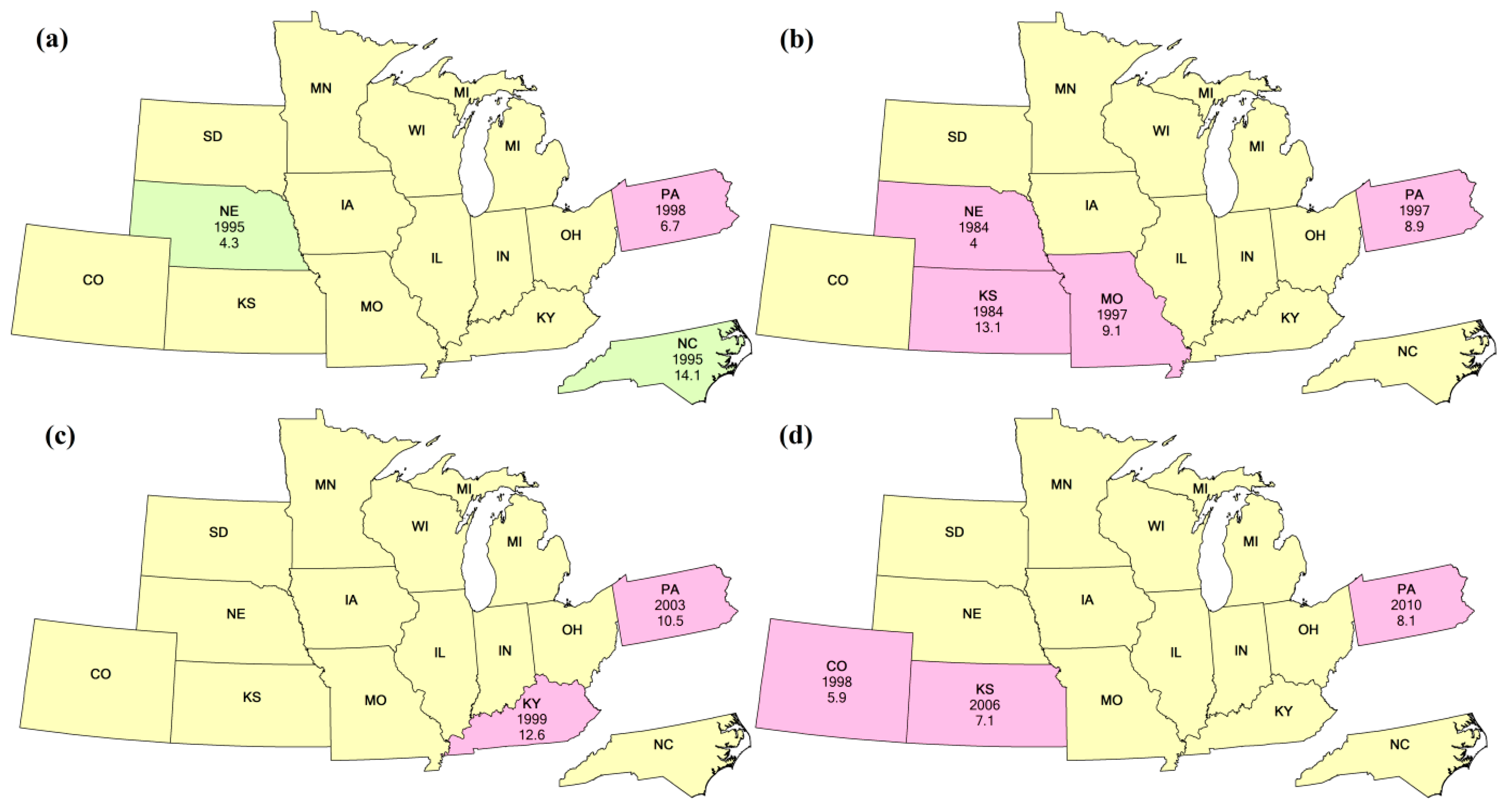
3.1. Planted Stage
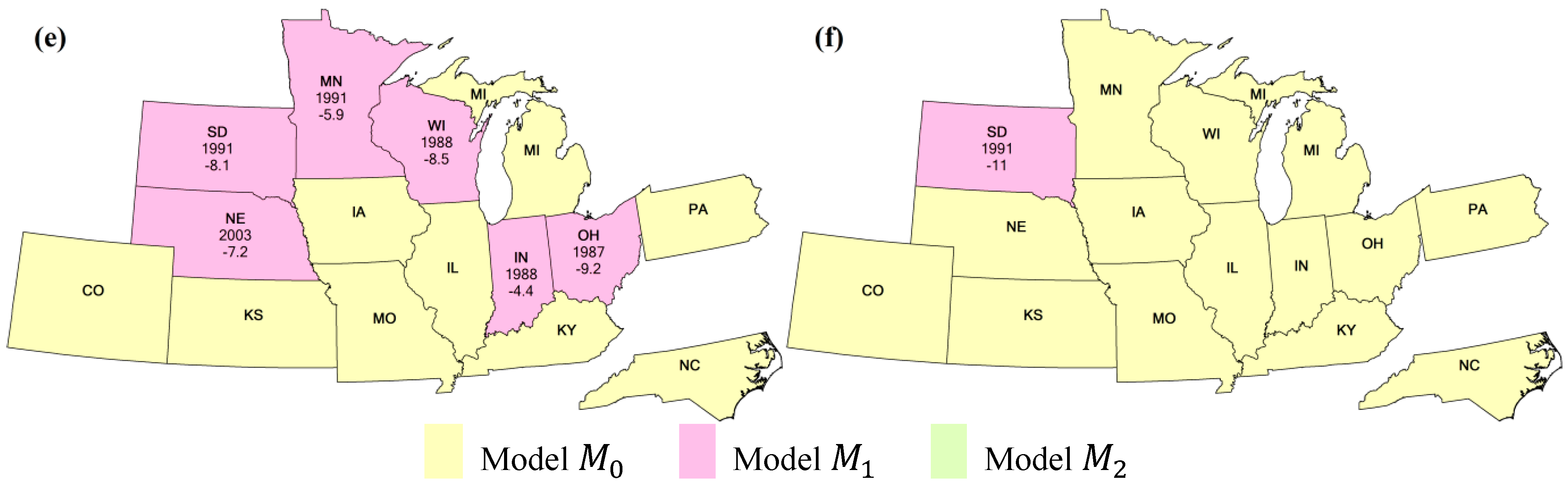
3.2. Silking/Blooming Stage
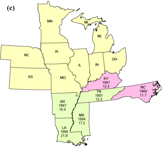
3.3. Mature/Dropping Leaves Stage
3.4. Duration of Vegetative Period
3.5. Duration of Reproductive Period
3.6. Duration of Growing Season
4. Discussion
4.1. Drivers of Crop Phenological Changes
4.2. Comparison of Different Methods
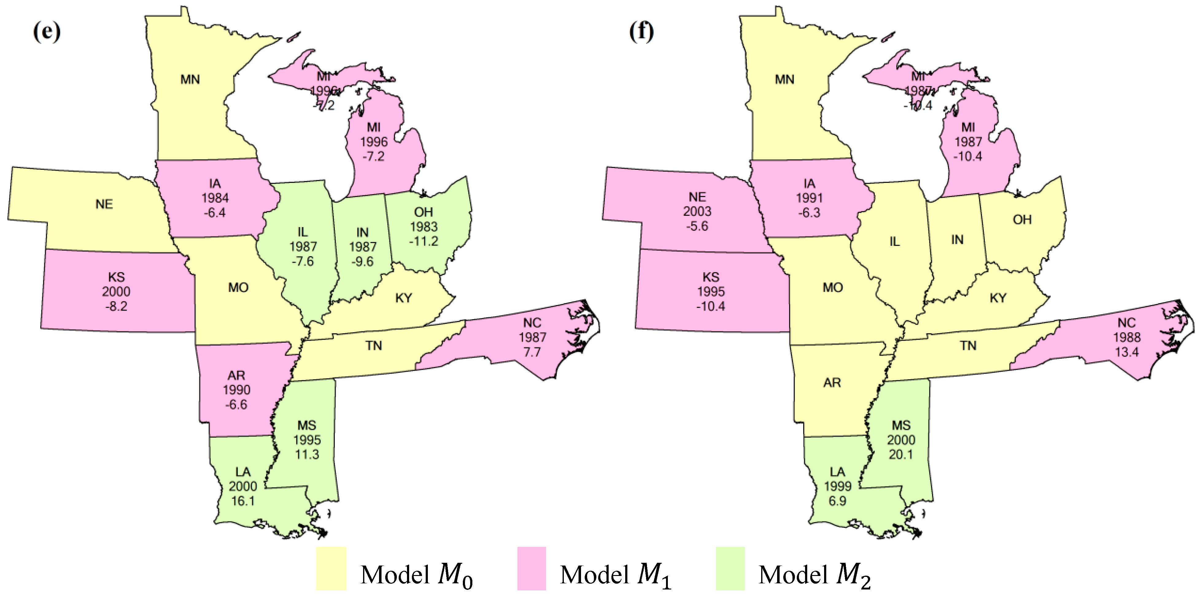
| No | State | Planted | Silking | Mature | Vegetative | Reproductive | Growing Season | ||||||||||||
|---|---|---|---|---|---|---|---|---|---|---|---|---|---|---|---|---|---|---|---|
| BP | PE | BC | BP | PE | BC | BP | PE | BC | BP | PE | BC | BP | PE | BC | BP | PE | BC | ||
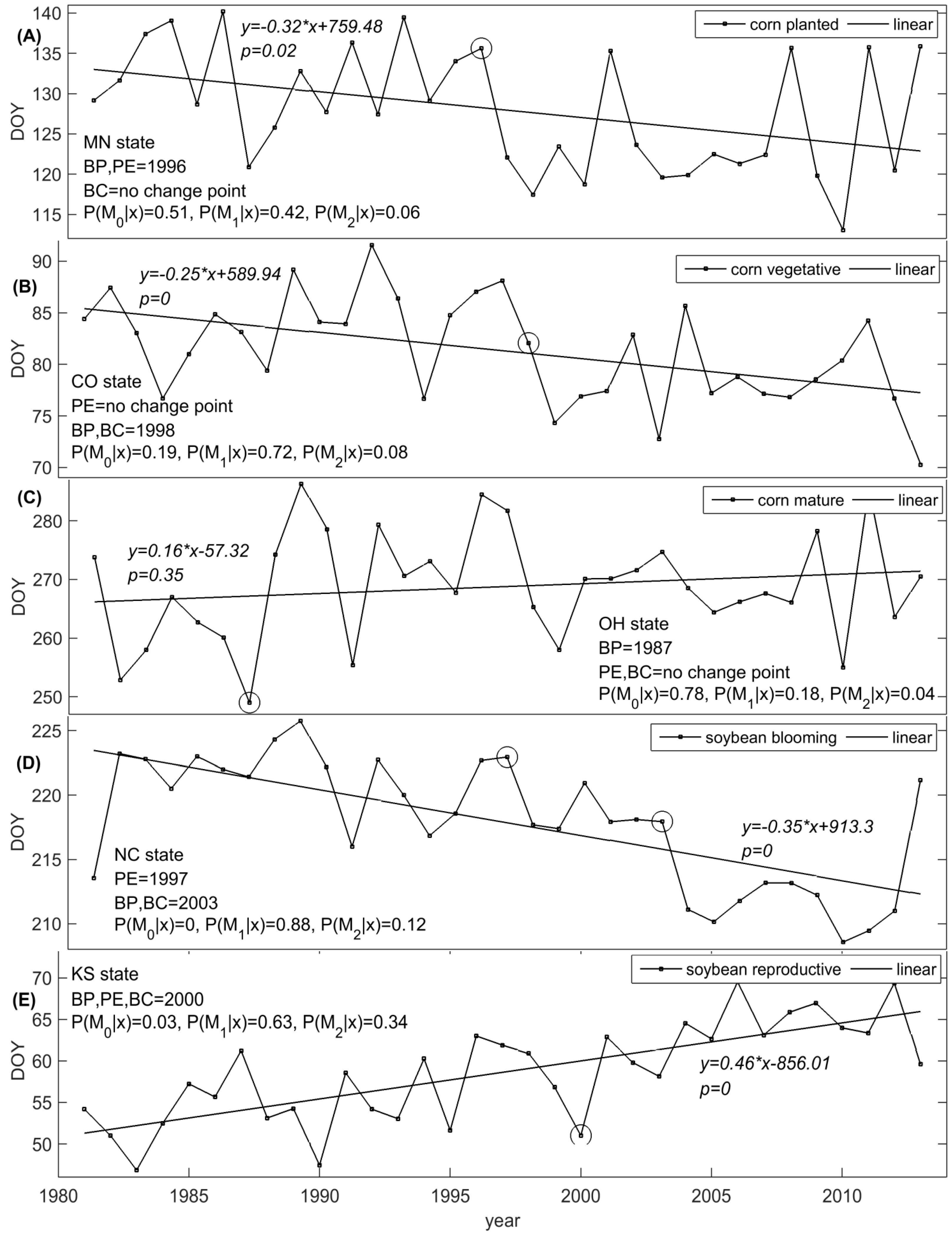
| 1 | CO | - | - | - | 1995 | 1997 | - | - | - | - | 1998 | - | 1998 | - | - | - | 1998 | 1998 | - |
| 2 | IL | - | - | - | - | - | - | 1988+ | - | - | - | - | - | 1988+ | - | - | - | - | - |
| 3 | IN | - | - | - | - | - | - | - | - | - | - | - | - | 1988+ | 2002 | 1988 | 1987 | - | - |
| 4 | IA | 1995 | 1996 | - | - | - | - | - | - | - | - | - | - | 2003+ | - | - | - | - | - |
| 5 | KS | 1985 | - | - | 1984+ | 1997/1999 | 1984 | - | - | - | 2006 | 2006 | 2006 | - | - | - | - | - | - |
| 6 | KY | 1998 | 1998 | - | 1998+ | 1998 | - | 1999 | 1999 | 1999 | - | - | - | - | - | - | - | - | - |
| 7 | MI | - | - | - | 2004 | 2004 | - | - | - | - | - | - | - | 1985 | - | - | - | - | - |
| 8 | MN | 1996 | 1996 | - | 1997 | 1996 | - | 1989+ | - | - | - | - | - | 1991 | 1995 | 1991 | 1991 | 1991 | - |
| 9 | MO | - | 1999 | - | 1997 | 1997 | 1997 | - | 1997 | - | - | - | - | - | - | - | - | - | - |
| 10 | NE | 1984 | 1995 | 1995 | 1997 | 1997 | 1984 | - | - | - | - | - | - | 2003 | 2003 | 2003 | - | - | - |
| 11 | NC | 1985 | 1996 | 1995 | - | 1995 | - | - | - | - | - | - | - | 1996+ | - | - | - | 1996 | - |
| 12 | OH | - | - | - | - | - | - | 1987 | - | - | - | - | - | 1987 | 1987 | 1987 | 1987 | - | - |
| 13 | PA | 1998 | 1998 | 1998 | 1997+ | 1997 | 1997 | 2003 | 2000 | 2003 | 2010 | - | 2010 | - | - | - | - | - | - |
| 14 | SD | 1999 | 1997 | - | - | - | - | 1991+ | 1991 | - | - | - | - | 1991 | 1991 | 1991 | 1991 | 1991 | 1991 |
| 15 | WI | 1996 | 1996 | - | - | - | - | 1988+ | - | - | 2010 | - | - | 1988 | 1991 | 1988 | 1991 | 1991 | - |
| No | State | Planted | Blooming | Dropping Leaves | Vegetative | Reproductive | Growing Season | ||||||||||||
|---|---|---|---|---|---|---|---|---|---|---|---|---|---|---|---|---|---|---|---|
| BP | PE | BC | BP | PE | BC | BP | PE | BC | BP | PE | BC | BP | PE | BC | BP | PE | BC | ||
| 1 | AR | 1995 | 1993 | 1995 | 1997+ | 1997 | 1997 | 1997 | 1997 | 1997 | 2001+ | 1997/2001 | 2001 | 1990+ | 1991 | 1990 | 1984 | - | - |
| 2 | IL | - | - | - | 1984 | - | 2009 | - | - | - | - | - | 2001 | 1987 | - | 1987 | - | - | - |
| 3 | IN | - | - | - | 1987 | - | 2011 | - | - | - | - | - | - | 1987 | - | 1987 | - | - | - |
| 4 | IA | 1996 | 1996 | - | - | - | - | - | - | - | - | - | - | 1984 | 1998 | 1984 | 1991 | 1995 | 1991 |
| 5 | KS | 1997+ | 1996 | 1996 | 1995+ | 1995 | 1995 | - | - | - | + | - | - | 2000+ | 2000 | 2000 | 1995+ | 1995 | 1995 |
| 6 | KY | 1998 | 1998 | 1998 | 1998 | 1998 | 1998 | 1997 | 1997 | 1997 | - | - | - | 1994 | 1994 | - | - | - | - |
| 7 | LA | 2003 | 1995 | 2003 | + | - | - | 1995+ | 1995 | 1995 | 2005 | - | 2005 | 2005+ | - | 2000 | 1998+ | 1997/1998 | 1999 |
| 8 | MI | - | - | - | 1997 | 1997 | 1997 | - | - | - | - | - | - | 1996+ | 1996 | 1996 | 1987 | 1987 | 1987 |
| 9 | MN | - | - | - | - | - | - | - | - | - | - | - | - | - | - | - | - | - | - |
| 10 | MS | 1993 | 1993 | 1993 | + | - | - | 1993+ | 1993/1994 | 1994 | 2006 | - | 1995 | 2006+ | - | 1995 | - | - | 2000 |
| 11 | MO | - | - | - | - | - | - | 2007+ | - | - | 1996 | 1996 | - | - | - | - | - | - | - |
| 12 | NE | 1996+ | 1996 | 1996 | 1997 | - | - | 1985 | - | - | 1988 | 1988 | 1988 | 2003+ | - | - | 1996 | 1996 | 2003 |
| 13 | NC | - | - | - | 2003 | 1997 | 2003 | 1989+ | 1997 | 1989 | 2002 | 2002 | 2002 | 1987+ | 1988 | 1987 | 1988 | 1994 | 1988 |
| 14 | OH | - | - | - | 1984 | 1990 | - | - | - | - | - | - | 2011 | 1984 | - | 1983 | - | - | - |
| 15 | TN | 1998 | 1998 | 1998 | 2000+ | 1998 | 2000 | 1997+ | 1997 | 1997 | - | - | - | - | - | - | - | - | - |
5. Conclusions
Acknowledgments
Author Contributions
Conflicts of Interest
References
- Sacks, W.; Kucharik, C. Crop management and phenology trends in the us corn belt: Impacts on yields, evapotranspiration and energy balance. Agric. For. Meteorol. 2011, 151, 882–894. [Google Scholar] [CrossRef]
- Kucharik, C.J. Contribution of planting date trends to increased maize yields in the central United States. Agron. J. 2008, 100, 328–336. [Google Scholar] [CrossRef]
- Tao, F.; Yokozawa, M.; Xu, Y.; Hayashi, Y.; Zhang, Z. Climate changes and trends in phenology and yields of field crops in China, 1981–2000. Agric. For. Meteorol. 2006, 138, 82–92. [Google Scholar] [CrossRef]
- Liu, Y.; Xie, R.; Hou, P.; Li, S.; Zhang, H.; Ming, B.; Long, H.; Liang, S. Phenological responses of maize to changes in environment when grown at different latitudes in China. Field Crops Res. 2013, 144, 192–199. [Google Scholar] [CrossRef]
- Wang, J.; Wang, E.; Feng, L.; Yin, H.; Yu, W. Phenological trends of winter wheat in response to varietal and temperature changes in the North China Plain. Field Crops Res. 2013, 144, 135–144. [Google Scholar] [CrossRef]
- Ahas, R.; Aasa, A.; Menzel, A.; Fedotova, V.G.; Scheifinger, H. Changes in European spring phenology. Int. J. Climatol. 2002, 22, 1727–1738. [Google Scholar] [CrossRef]
- Spiertz, H. Challenges for crop production research in improving land use, productivity and sustainability. Sustainability 2013, 5, 1632–1644. [Google Scholar] [CrossRef]
- Coulibaly, J.; Gbetibouo, G.; Kundhlande, G.; Sileshi, G.; Beedy, T. Responding to crop failure: Understanding farmers’ coping strategies in Southern Malawi. Sustainability 2015, 7, 1620–1636. [Google Scholar] [CrossRef]
- Ma, X.; Huete, A.; Yu, Q.; Coupe, N.R.; Davies, K.; Broich, M.; Ratana, P.; Beringer, J.; Hutley, L.B.; Cleverly, J.; et al. Spatial patterns and temporal dynamics in savanna vegetation phenology across the North Australian tropical transect. Remote Sens. Environ. 2013, 139, 97–115. [Google Scholar] [CrossRef]
- Kucharik, C.J. A multidecadal trend of earlier corn planting in the central USA. Agron. J. 2006, 98, 1544–1550. [Google Scholar] [CrossRef]
- Bertin, R.I. Plant phenology and distribution in relation to recent climate change. J. Torrey Bot. Soc. 2008, 135, 126–146. [Google Scholar] [CrossRef]
- White, M.A.; de Beurs, K.M.; Didan, K.; Inouye, D.W.; Richardson, A.D.; Jensen, O.P.; O’Keefe, J.; Zhang, G.; Nemani, R.R.; van Leeuwen, W.J.D.; et al. Intercomparison, interpretation, and assessment of spring phenology in North America estimated from remote sensing for 1982–2006. Glob. Chang. Biol. 2009, 15, 2335–2359. [Google Scholar] [CrossRef]
- Cleland, E.E.; Chuine, I.; Menzel, A.; Mooney, H.A.; Schwartz, M.D. Shifting plant phenology in response to global change. Trends Ecol. Evol. 2007, 22, 357–365. [Google Scholar] [CrossRef] [PubMed]
- Chen, B.; Xu, G.; Coops, N.C.; Ciais, P.; Innes, J.L.; Wang, G.; Myneni, R.B.; Wang, T.; Krzyzanowski, J.; Li, Q.; et al. Changes in vegetation photosynthetic activity trends across the asia-pacific region over the last three decades. Remote Sens. Environ. 2014, 144, 28–41. [Google Scholar] [CrossRef]
- Dose, V.; Menzel, A. Bayesian analysis of climate change impacts in phenology. Glob. Chang. Biol. 2004, 10, 259–272. [Google Scholar] [CrossRef]
- Schleip, C.; Menzel, A.; Estrella, N.; Dose, V. The use of bayesian analysis to detect recent changes in phenological events throughout the year. Agric. For. Meteorol. 2006, 141, 179–191. [Google Scholar] [CrossRef]
- Kim, C.; Suh, M.-S.; Hong, K.-O. Bayesian changepoint analysis of the annual maximum of daily and subdaily precipitation over South Korea. J. Clim. 2009, 22, 6741–6757. [Google Scholar] [CrossRef]
- Xiong, L.; Guo, S. Trend test and change-point detection for the annual discharge series of the Yangtze river at the Yichang hydrological station/test de tendance et détection de rupture appliqués aux séries de débit annuel du fleuve Yangtze à la station hydrologique de Yichang. Hydrol. Sci. J. 2004, 49, 99–112. [Google Scholar]
- Perreault, L. Bayesian change-point analysis in hydrometeorological time series. Part 1. The normal model revisited. J. Hydrol. 2000, 235, 221–241. [Google Scholar] [CrossRef]
- Chu, P.-S.; Zhao, X. Bayesian change-point analysis of tropical cyclone activity: The central north pacific case. J. Clim. 2004, 17, 4893–4901. [Google Scholar] [CrossRef]
- Perreault, L.; Bernier, J.; Bobée, B.; Parent, E. Bayesian change-point analysis in hydrometeorological time series. Part 2. Comparison of change-point models and forecasting. J. Hydrol. 2000, 235, 242–263. [Google Scholar] [CrossRef]
- USDA/NASS. Quick Stats 2.0. Available online: http://quickstats.nass.usda.gov/ (accessed on 25 May 2015).
- USDA/NASS. National Crop Progress—Terms and Definitions. Available online: http://www.nass.usda.gov/Publications/National_Crop_Progress/Terms_and_Definitions/index.asp (accessed on 30 January 2014).
- Fehr, W.R.; Caviness, C.E.; Burmood, D.T.; Pennington, J.S. Stage of development descriptions for soybeans, glycine max (l.) merrill1. Crop Sci. 1971, 11, 929–931. [Google Scholar] [CrossRef]
- Kahaner, D.; Moler, C.; Nash, S. Numerical Methods and Software; Prentice Hall: Upper Saddle River, NJ, USA, 1988. [Google Scholar]
- Shen, Y.; Di, L.; Yu, G.; Wu, L. Correlation between corn progress stages and fractal dimension from modis-ndvi time series. Geosci. Remote Sens. Lett. IEEE 2013, 10, 1065–1069. [Google Scholar] [CrossRef]
- Schwarz, J.; Staenz, K. Adaptive threshold for spectral matching of hyperspectral data. Can. J. Remote Sens. 2001, 27, 216–224. [Google Scholar] [CrossRef]
- Perreault, L.; Parent, É.; Bernier, J.; Bobée, B.; Slivitzky, M. Retrospective multivariate bayesian change-point analysis: A simultaneous single change in the mean of several hydrological sequences. Stoch. Environ. Res. Risk Assess. 2000, 14, 243–261. [Google Scholar] [CrossRef]
- Jordan, M.I. Bayesian modeling and inference, lecture 6: Jeffreys priors. 2010. Available online: http://www.cs.berkeley.edu/~jordan/courses/260-spring10/lectures/lecture6.pdf (accessed on 25 May 2015).
- Berger, J.O. Statistical Decision Theory and Bayesian Analysis; Springer-Verlag: New York, NY, USA, 1985. [Google Scholar]
- Berger, J.O.; Pericchi, L.R.; Ghosh, J.K.; Samanta, T.; Santis, F.D.; Berger, J.O.; Pericchi, L.R. Objective bayesian methods for model selection: Introduction and comparison. Lect. Notes Monogr. Ser. 2001, 38, 135–207. [Google Scholar]
- Son, Y.S.; Kim, S.W. Bayesian single change point detection in a sequence of multivariate normal observations. Statistics 2005, 39, 373–387. [Google Scholar] [CrossRef]
- Berger, J.O.; Pericchi, L.R. The intrinsic bayes factor for model selection and prediction. J. Am. Stat. Assoc. 1996, 91, 109–122. [Google Scholar] [CrossRef]
- Berger, J.O.; Pericchi, L.R. Accurate and stable bayesian model selection: The median intrinsic bayes factor. Sankhya B 1998, 60, 1–18. [Google Scholar]
- Bernardo, J.M.; Simith, A.F.M. Bayesian Theory; Wiley: New York, NY, USA, 1994. [Google Scholar]
- Bruns, H.; Abbas, H. Planting date effects on bt and non-bt corn in the mid-south USA. Agron. J. 2006, 98, 100–106. [Google Scholar] [CrossRef]
- Xiao, D.; Tao, F. Contributions of cultivars, management and climate change to winter wheat yield in the North China Plain in the past three decades. Eur. J. Agron. 2014, 52, 112–122. [Google Scholar] [CrossRef]
- Fernandez-Cornejo, J.; Caswell, M. The first decade of genetically engineered crops in the United States. Econ. Inf. Bull. 2006, 11, 1–30. [Google Scholar]
- James, C. Global status of transgenic crops in 1997. In The International Service for the Acquisition of Agri-Biotech Applications (ISAAA) Briefs; ISAAA: Ithaca, NY, USA, 1997; Volume 5, pp. 1–31. [Google Scholar]
- Gesch, R.W.; Archer, D.W. Influence of sowing date on emergence characteristics of maize seed coated with a temperature-activated polymer. Agron. J. 2005, 97, 1543–1550. [Google Scholar] [CrossRef]
- Heatherly, L.G. Early soybean production system (ESPS). In Soybean Production in the Midsouth; Heatherly, L.G., Hodges, H.F., Eds.; CRC Press: Boca Raton, FL, USA, 1999; pp. 103–118. [Google Scholar]
- Muchow, R.C.; Carberry, P.S. Environmental control of phenology and leaf growth in a tropically adapted maize. Field Crops Res. 1989, 20, 221–236. [Google Scholar] [CrossRef]
- Shen, Y.; Wu, L.; Di, L.; Yu, G.; Tang, H.; Yu, G.; Shao, Y. Hidden markov models for real-time estimation of corn progress stages using modis and meteorological data. Remote Sens. 2013, 5, 1734–1753. [Google Scholar] [CrossRef]
- Van Diepen, C.A.; Wolf, J.; van Keulen, H.; Rappoldt, C. Wofost: A simulation model of crop production. Soil Use Manag. 1989, 5, 16–24. [Google Scholar] [CrossRef]
- Brinkman, R.; Sombroek, W.G. The effects of global change on soil conditions in relation to plant growth and food production. In Global Climate Change and Agricultural Production: Direct and Indirect Effects of Changing Hydrological, Pedological and Plant Physiological Processes; Bazzaz, F., Sombroek, W., Eds.; Wiley: Chichester, NH, USA, 1996; pp. 141–169. [Google Scholar]
- Wang, X.; Piao, S.; Ciais, P.; Li, J.; Friedlingstein, P.; Koven, C.; Chen, A. Spring temperature change and its implication in the change of vegetation growth in North America from 1982 to 2006. Proc. Natl. Acad. Sci. USA 2011, 108, 1240–1245. [Google Scholar] [CrossRef] [PubMed]
- Desclaux, D.; Roumet, P. Impact of drought stress on the phenology of two soybean (glycine max l. Merr) cultivars. Field Crops Res. 1996, 46, 61–70. [Google Scholar] [CrossRef]
- Gu, L.; Hanson, P.J.; Post, W.M.; Kaiser, D.P.; Yang, B.; Nemani, R.; Pallardy, S.G.; Meyers, T. The 2007 Eastern US spring freeze: Increased cold damage in a warming world? BioScience 2008, 58, 253–262. [Google Scholar] [CrossRef]
- Nielsen, R.L. Historical Corn Grain Yields for Indiana and the U.S. Department of Agronomy. Available online: http://www.agry.purdue.edu/ext/corn/news/timeless/YieldTrends.html (accessed on 6 September 2014).
- Waha, K.; Müller, C.; Bondeau, A.; Dietrich, J.P.; Kurukulasuriya, P.; Heinke, J.; Lotze-Campen, H. Adaptation to climate change through the choice of cropping system and sowing date in Sub-saharan Africa. Glob. Environ. Chang. 2013, 23, 130–143. [Google Scholar] [CrossRef]
- Lauer, J.; Carter, P.; Wood, T.; Diezel, G.; Wiersma, D.; Rand, R.; Mlynarek, M. Corn hybrid response to planting date in the northern corn belt. Agron. J. 1999, 91, 834–839. [Google Scholar] [CrossRef]
- Pettitt, A.N. A non-parametric approach to the change-point problem. Appl. Stat. 1979, 28, 126–135. [Google Scholar] [CrossRef]
- Bai, J.; Perron, P. Computation and analysis of multiple structural change models. J. Appl. Econom. 2003, 18, 1–22. [Google Scholar] [CrossRef]
- Zeileis, A.; Kleiber, C.; Krämer, W.; Hornik, K. Testing and dating of structural changes in practice. Comput. Statt. Data Anal. 2003, 44, 109–123. [Google Scholar] [CrossRef]
- Wijngaard, J.B.; Klein Tank, A.M.G.; Können, G.P. Homogeneity of 20th century European daily temperature and precipitation series. Int. J. Climatol. 2003, 23, 679–692. [Google Scholar] [CrossRef]
© 2015 by the authors; licensee MDPI, Basel, Switzerland. This article is an open access article distributed under the terms and conditions of the Creative Commons Attribution license (http://creativecommons.org/licenses/by/4.0/).
Share and Cite
Shen, Y.; Liu, X. Phenological Changes of Corn and Soybeans over U.S. by Bayesian Change-Point Model. Sustainability 2015, 7, 6781-6803. https://doi.org/10.3390/su7066781
Shen Y, Liu X. Phenological Changes of Corn and Soybeans over U.S. by Bayesian Change-Point Model. Sustainability. 2015; 7(6):6781-6803. https://doi.org/10.3390/su7066781
Chicago/Turabian StyleShen, Yonglin, and Xiuguo Liu. 2015. "Phenological Changes of Corn and Soybeans over U.S. by Bayesian Change-Point Model" Sustainability 7, no. 6: 6781-6803. https://doi.org/10.3390/su7066781
APA StyleShen, Y., & Liu, X. (2015). Phenological Changes of Corn and Soybeans over U.S. by Bayesian Change-Point Model. Sustainability, 7(6), 6781-6803. https://doi.org/10.3390/su7066781