Article

Research on the Multi-Period Small-Signal Stability Probability of a Power System with Wind Farms Based on the Markov Chain

1
Electrical and Electronic Engineering Institute, North China Electric Power University, Mailbox 435, No. 2 Beinong Road, Changping District, Beijing 102206, China
2
Gansu Electrical Power Research Institute, No.8 Binhe East Road, Chengguan North District, Lanzhou 730030, China
*
Author to whom correspondence should be addressed.
These authors contributed equally to this work.
Sustainability 2015, 7(4), 4582-4599; https://doi.org/10.3390/su7044582
Submission received: 13 January 2015 / Revised: 7 April 2015 / Accepted: 9 April 2015 / Published: 17 April 2015
(This article belongs to the Special Issue Sustainability in Electrical Engineering)

Abstract

:
In the traditional studies on small-signal stability probability of a power system with wind farms, the frequency of wind speed was often assumed to obey to some extent a particular probability distribution. The stability probability that is thus obtained, however, actually only reflects the power system stability characteristics on long time scales. In fact, there is a direct correlation between the change of wind speed and the current state of wind speed, resulting in the system stability characteristics in different time periods having a great difference compared with that of long time scales. However, the dispatchers are more concerned about the probability that the power system remains stable in the next period or after several periods, namely the stability characteristics of the power system in a short period or multi-period. Therefore, research on multi-period small-signal stability probability of a power system with wind farms has important theoretical value and practical significance. Based on the Markov chain, this paper conducted in-depth research on this subject. Firstly, the basic principle of the Markov chain was introduced, based on which we studied the uncertainty of wind power by adopting the transition matrix and the wind speed−power output transformation model and established the probability distribution model of multi-period wind power. Then the boundary-based small-signal stability probability evaluation method was used to establish an evaluation model of multi-period small-signal stability probability of power system with wind farms. Finally, taking the power system with two wind farms as an example, we analyzed its small-signal stability probability and studied the influence of the initial states of wind speed and different periods on the probability of stability. This study provides a new method and support for analyzing the small-signal stability probability of a power system with wind farms.

1. Introduction

With the aggravation of the energy crisis, increasingly prominent environmental problems and the rapid development of wind power generation technology [1,2], large-scale wind power integration has become an important trend in the development of new energy resources. However, wind turbine energy differs greatly from conventional units [3] in structure and its output has characteristics of randomness and volatility affected by wind speed. The above characteristics of wind power integration make the analysis, operation, and control of the power system more complex. Among those problems, the small-signal stability probability of the power system has become the focus of universal concern.
To date, many papers have researched this subject. Most of the papers [4,5,6] are based on one or a set of deterministic scenarios and draw conclusions through the comparison of changes of the system’s damping before and after wind power integration, which essentially belongs to deterministic research methods. However, this method fails to consider the effect of randomness and volatility of wind power. This limitation makes some scholars adopt the method of probability instead. Rueda et al. [7,8] considered the randomness of wind power and adopted the Monte Carlo method to analyze small-signal stability probability of the power system, which needs a great deal of sampling calculation and is very time consuming. Based on the Gram-Charlier series, eigenvalue sensitivity, and the volatility of wind speed, Bu et al. [9] studied small-signal stability probability of a power system with wind farms. Soleimanpour and Mohammadi [10] used the two-point estimating method to make a similar calculation. Based on the 2 m + 1 points estimating method, Cornish-Fisher expansion and considering the correlation of wind speed, Yue et al. [11] studied the probability of small-signal stability of the power system after wind power integration and adopted the Monte Carlo method to verify the results. Overall, these studies considered the random fluctuation of wind speed; the conclusions can therefore more fully describe the small-signal stability of a power system with wind power integration. However, an important premise of these conclusions is that wind speed frequency is assumed to obey approximately a certain probability distribution, such as the Weibull distribution [12]. However, the wind speed frequency distribution model is obtained by extensive historical wind speed data statistics and data fitting, reflecting the general distribution characteristics of wind speed over a very long statistical time period. The probability of small-signal stability obtained thus also reflects the stability characteristic of the power system on a long time scale. This is clearly not wrong, but the dispatchers are more concerned about the probability that the power system remains stable in the next period or after several periods, namely the stability characteristics of the power system in a short period or multi-time periods. At present, no paper has conducted research on this subject.
In fact, the change of wind speed is closely linked to its current state. Under normal circumstances, the conversion probability of wind speed to the adjacent wind speed is high, whereas the conversion probability to another wind speed is much lower. The change characteristic of wind speed will make the small-signal probabilistic stability on different time scales quite different from that on a long time scale. Therefore, the core of this research is to establish a model that can accurately reflect the law of multi-period wind speed transition. The Markov chain studies precisely the transition laws of states of things at different times, which has a good adaptability to the change of wind speed, thereby being suitable for modeling of the law of multi-period wind speed transition and research of small-signal stability probability of a power system with wind farms. Until now, the Markov chain has been used in an electric power system to a certain extent. Halilcevic et al. [13] forecasted the safety state of a power system based on the Markov chain. Li et al. [14] studied the combined power output of the new energy and battery energy storage system by using the Markov chain. Wang et al. [15] and Li et al. [16] adopted the Markov chain model to forecast the load and the output of the photovoltaic system. At present, there is no application of the Markov chain in small-signal stability of a power system.
Due to the above, this paper first introduced the founding principle of the Markov chain, upon which we based the uncertainty of wind power by adopting the transfer matrix and the wind speed-power output transformation model and established the probability distribution model of multi-period wind power. Then the boundary-based small-signal stability probability assessment method was used to establish an evaluation model of multi-period small-signal stability probability of a power system with wind farms. Finally, taking the power system with two wind farms as an example, we analyzed its small-signal stability probability and focused on the influence of the initial state of wind speed and different periods on the probability of stability. We subsequently compared it with the traditional small-signal probabilistic stability assessment methods to provide a new method and support for analyzing the small-signal stability probability of a power system with wind power integration.

2. The Markov Chain

A Markov chain is a discrete-time stochastic process with the Markov property. The Markov property is also characterized as memoryless: the next state depends only on the current state but not the sequence of events that preceded it. When the Markov chain is applied to research on the change laws of matter, we first get s discrete states X1, X2,…, Xs and reveal the matter’s intrinsic variation law and development trend in the future by the transition probability between each state. The transition probability is defined as P [ X n + 1 = j | X n = i ] = p i j , representing the probability of the system’s state transferring from Xi to Xj. For a system that has s states, the matrix formed by the transition probabilities between each state is:
P = [ p 11 p 1 s      p s 1 p s s ]
where the matrix P is called the one-step transition matrix with p i j 0 , and the total of matrix elements in each row is 1. According to the one-step transition matrix, we can analyze and predict the future state of things. Assuming the system state at time t is X(t) and according to the Markov chain, the distribution probability at time t + 1 is:
P = [ p 11 p 1 s      p s 1 p s s ]
Through the iteration, the distribution probability of the system state at time t + k is:
X(t + k) = X(t)Pk
where Pk is called k-step transition matrix. Under normal circumstances, Pk changes with k. However, for the aperiodic and irreducible transition matrix [17,18], when k approaches infinity (k→∞), the Markov chain will reach a limit state. At this point, each row in the matrix Pk is the same and the values of all the elements in the matrix will no longer change. Then for any initial state of the system X(t) (Each component of the vector is non-negative and their total is 1), the calculated X(t + k) remains unchanged, i.e., X(t + k) reaches a stationary distribution which is independent of the initial state. The one-step transition matrix of wind speed in the paper just belongs to this case. Obviously, the condition that k approaches infinity (k→∞) exists only in theory. In the practically acceptable range, when k increases to a certain extent, each row in the Pk is basically the same, and the values of all the elements no longer change, which can thus be regarded as the limit state.

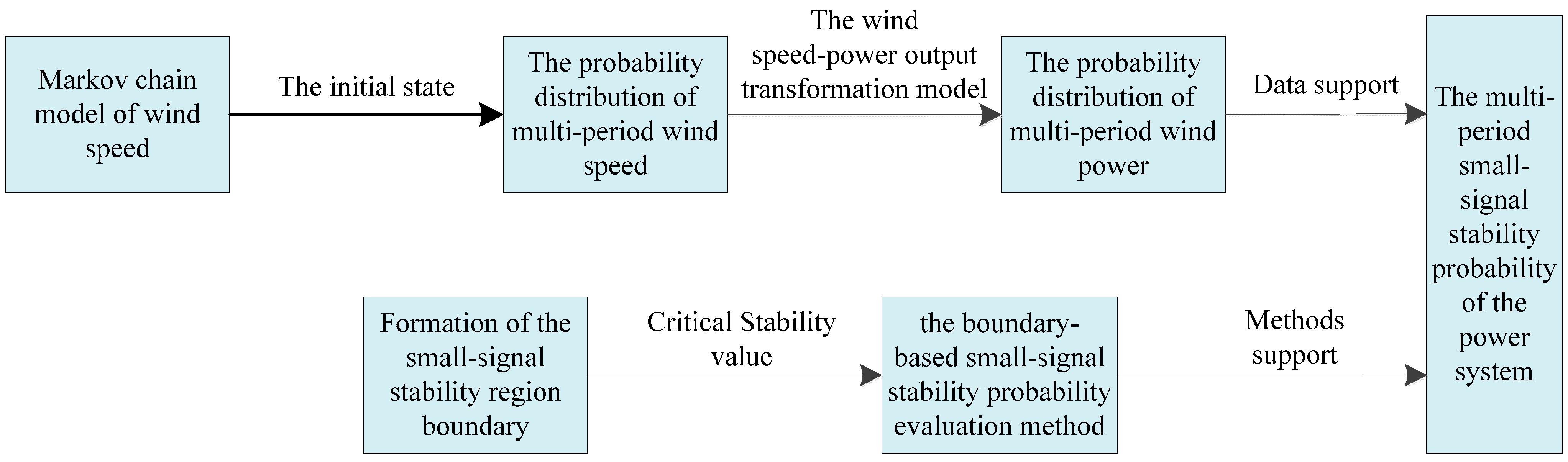
3. Uncertainty Modeling of Wind Power Based on the Markov Chain

The change of wind speed has the Markov property, which is a typical stochastic process. Using the Markov chain to describe the change of wind speed, and through the establishment of transition matrix of wind speed’s states, we can analyze the wind power’s transfer process of uncertainty, so as to establish probability distribution models for wind speed and wind power in multi-time periods.

3.1. The Markov Property of Wind Speed

Current studies point out that wind speed has the Markov property and even the method of the Markov chain has become one of the typical methods to generate wind speed time series. Shamshad et al. [19] and Castro et al. [20] analyzed and verified the Markov property of wind speed based on large amount of historical data, and through simulation they obtained the wind speed time series which bears a strong similarity to the actual wind speed. Nicola et al. [21] combined the Markov chain method and Monte Carlo method to generate wind speed time series. The research of Hocaoglu et al. [22] showed that when the Markov chain is applied to generate the data of wind speed, the increase of the number of states will make the generated wind speed data closer to the real data.

3.2. The Establishment of Transition Matrix

For the Markov chain, the transition matrix between each state can be obtained by the historical statistical data. The more historical data we get, the better practical variation laws of each state can be reflected by the results. The specific steps of establishing the transition matrix between each state are as follows:
(1)
The state division of wind speed: for single wind farm, random variables are the wind speeds for the wind farm, where wind speeds are divided into s discrete intervals. For multi wind farms, wind speeds of each wind farm are random variables. Considering the influence of geographical and environmental factors, wind speeds of each wind farm in the same area often have a certain correlation. Then we can combine the states of each wind farm’s wind speed and make use of the transition probability to reflect the correlation relationship. That is, the statistical transition probabilities obtained will be different if the correlations are different. Assume n wind farms, the number of wind speed states of which are s1, s2, …, sn respectively. Then the total number of the system’s states is
s = i = 1 n s i
(2)
Historical wind speed data statistics: set the historical wind speed data as sample data, judge which state the sample data belongs to according to the state division of wind speed, calculate statistics of the number of times (Nij) that the wind speed’s state transfers from Xi to Xj in adjacent time, and obtain the transition frequency matrix:
N = [ N 11 N 1 s      N s 1 N s s ]
(3)
The establishment of the transition matrix: according to the definition of transition probability we can get:
p ij = N ij / j = 1 s N i j
Thus, the transition matrix P between each wind speed state is obtained.
(4)
The establishment of multi-step transition matrix: according to the definition of multi-step transition matrix, we can get the k-step transition matrix Pk after iterating matrix P for k times.

3.3. The Probability Distribution Model of Multi-period Wind Speed

After we get the transition matrix between each wind speed state, combined with the initial distribution of wind speed and according to Equations (2) and (3), we can forecast the probability distribution of wind speed in multi time periods. Equations (2) and (3) are just the probability distribution model of multi-period wind speed.

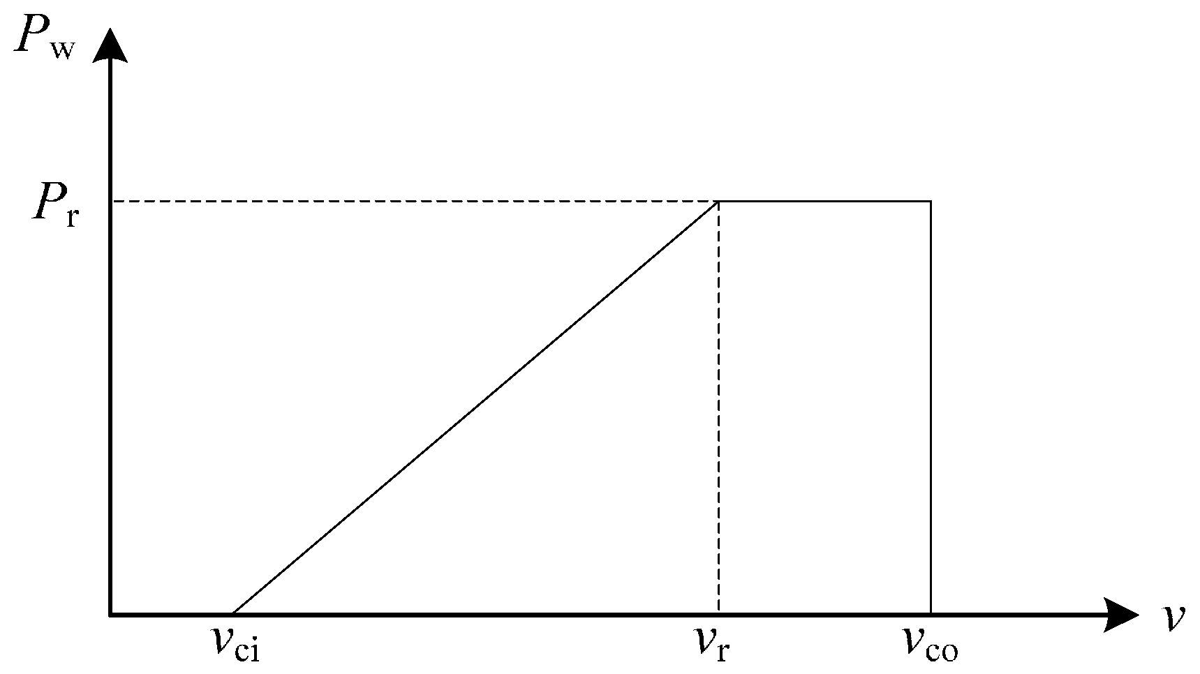
3.4. The Probability Distribution Model of Multi-period Wind Power

According to the wind speed-power curve of wind turbines, wind speed can be converted to the corresponding wind power. In general, the conversion between wind power and wind speed can approximately be represented by the curve [23] shown in Figure 1.
Figure 1. The wind speed-power characteristic curve of wind turbines.
Sustainability 07 04582 g001
Expression for the characteristic curve is:
P w = { 0 v < v c i o r v > v c o v v c i v r v c i P r v c i v v r P r v r < v < v c o
In Equation (6), v is wind speed, Pw is the output of wind turbines. Pr, vci, vr, vco are respectively the rated power, cut-in wind speed, rated wind speed and cut-out wind speed of the wind turbines. The corresponding values for the parameters in this paper are 2 MW, 3 m/s, 12 m/s, 25 m/s, respectively.
Assuming the state and parameters of each wind turbine in the wind farm are the same, we used the lumped model to make them equivalent to a signal machine. Then the active power output of the equivalent wind turbine is:
Pfarm = NwPw
In which, Pfarm is the active power output of the equivalent wind turbine, Nw is the number of wind turbines in the wind farm.
Through the wind speed-power output transformation model defined by Equations (6) and (7) and the probability distribution of multi-period wind speed, we can get the probability distribution of multi-period wind power.

4. The Evaluation Model of Multi-Period Small-Signal Stability Probability of a Power System with Wind Farms

The probability distribution model of multi-period wind power in wind farms has been established above, and in this section we will apply it to the evaluation of small-signal stability probability. To determine the small-signal stability of the system, the method based on small-signal stability region boundary was adopted.

4.1. The Boundary-Based Small-Signal Stability Probability Evaluation Method

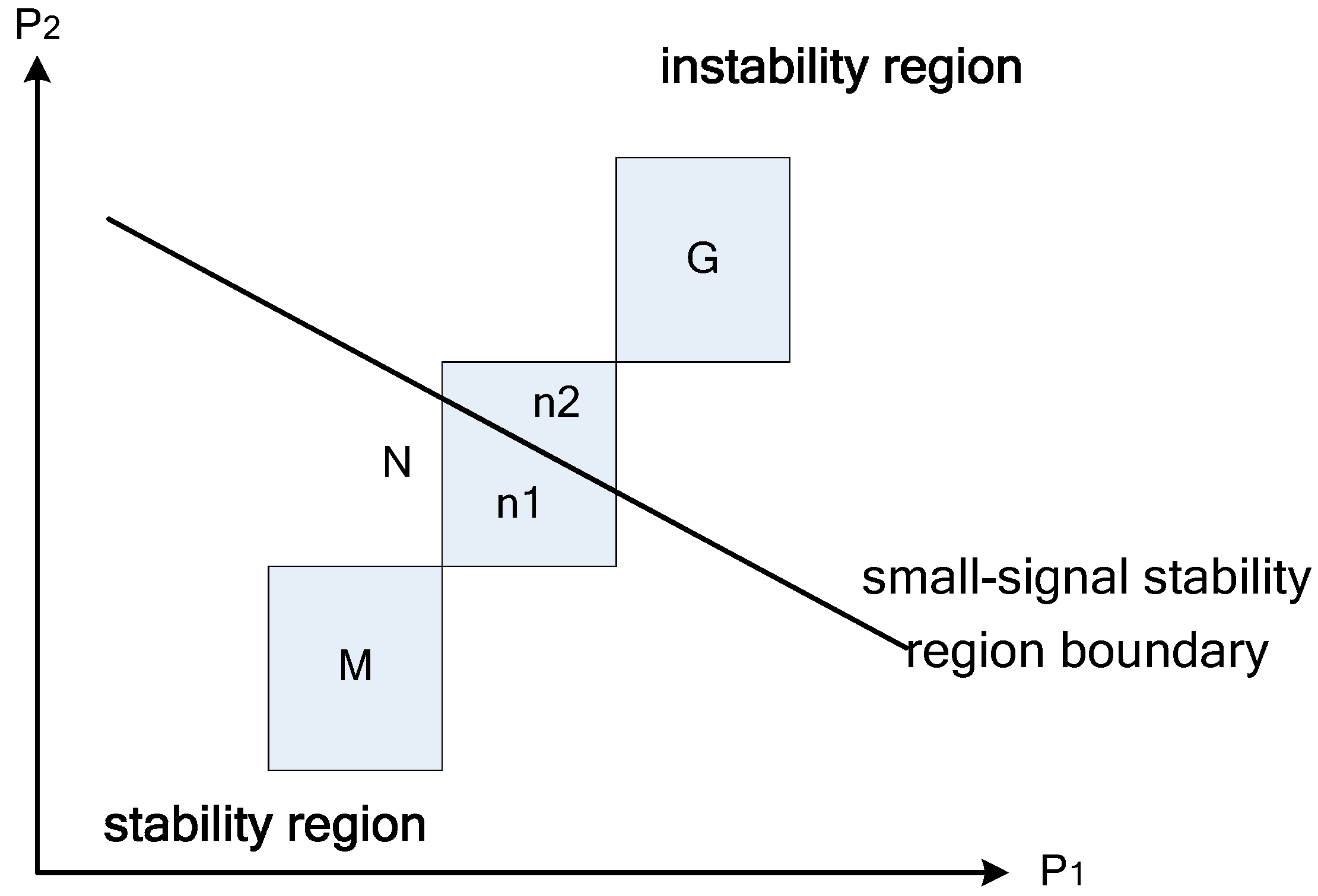
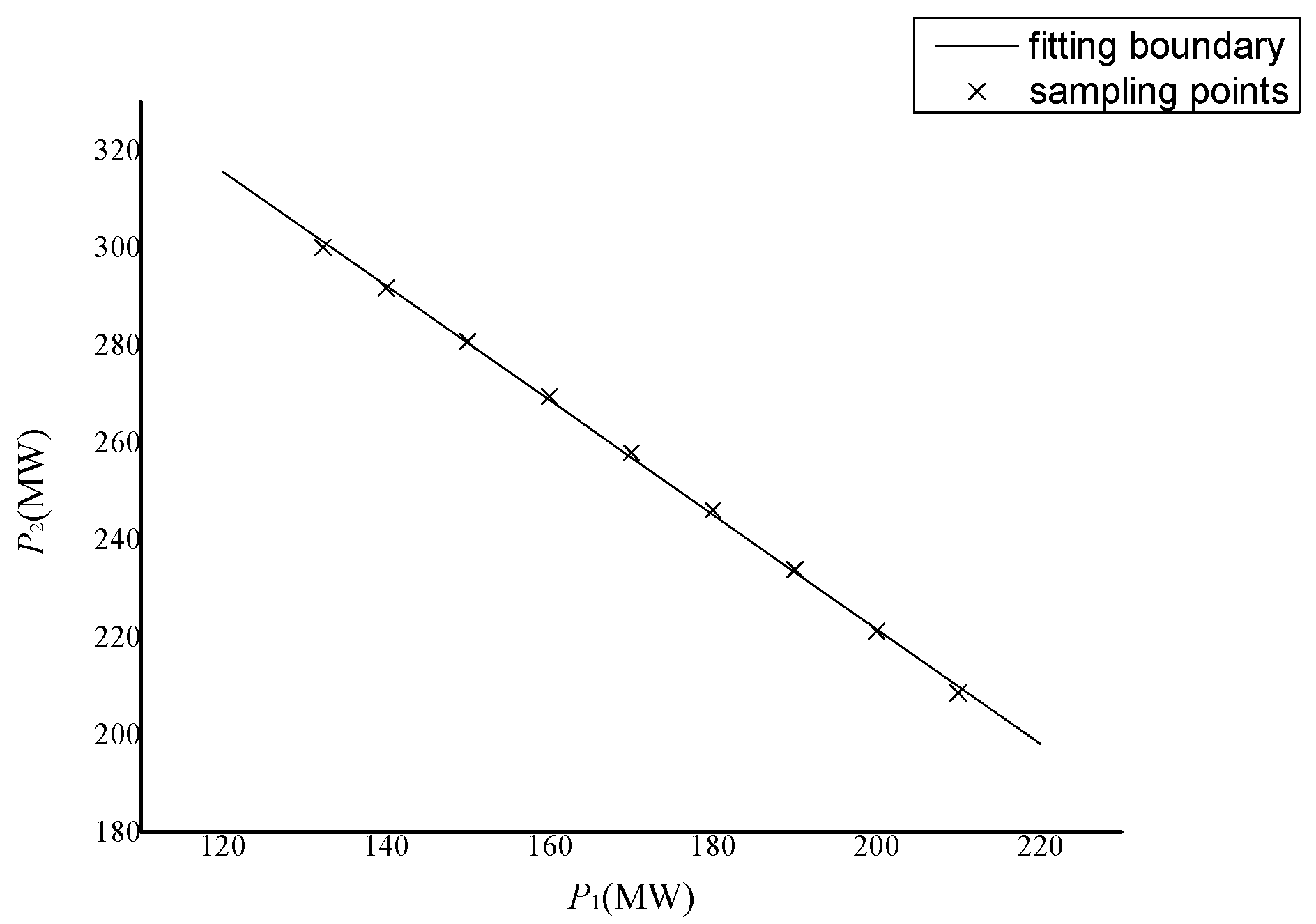
4.1.1. Small-signal Stability Region Boundary

The dynamics model of power systems can be described by a set of differential-algebraic equations:
{ x ˙ = f ( x , y , k ) 0 = g ( x , y , k )
In Equation (8), x∈Rn is the state variable of the system, n is the dimension of the state variable, y∈Rm is the algebraic variable, m is the dimension of the algebraic variable, k∈Rp is the system parameter and p is the dimension of the parameter.
At the equilibrium point (x0, y0, k0) of the power system, the equation set satisfies Equation (9).
{ f ( x 0 , y 0 , k 0 ) = 0 g ( x 0 , y 0 , k 0 ) = 0
Linearize Equation (9) and we get:
[ Δ x ˙ 0 ] = [ f x f y g x g y ] [ Δ x Δ y ]
in which
{ f x = f / x | ( x 0 , y 0 , k 0 ) f y = f / y | ( x 0 , y 0 , k 0 ) g x = g / x | ( x 0 , y 0 , k 0 ) g y = g / y | ( x 0 , y 0 , k 0 )
When the gy is nonsingular, the algebraic variables can be eliminated in Equation (10) and after arranging we get:
Δ x ˙ = J ( x , y , k ) Δ x
in which the formula of J is:
J ( x , y , k ) = f x f y g y 1 g x
In Equation (13) J is the characteristic matrix of the system. According to Lyapunov’s first theorem, the small-signal stability of the system is decided by the eigenvalues of the characteristic matrix J. When all of the real parts of the eigenvalues are less than zero, the system is stable under small disturbance. Under normal circumstances, the system can keep stable in operation. However, with the change of parameter k, three circumstances may appear in which the eigenvalue makes the system achieve critical conditions of the small-signal stability: (1) A pair of real eigenvalues cross the imaginary axis, causing saddle node bifurcation (SNB); (2) A pair of conjugate complex eigenvalues cross the imaginary axis, causing Hopf bifurcation (HB); and (3) Matrix gy is singular, causing singularity-induced bifurcation (SIB). Thus the small-signal stability region boundary ( Ω s s s r ) consists of these three types of point set.
Ω s s s r = { S N B s } { H B s } { S I B s }
In Equation (14), SNBs is the point set of SNB, HBs is the point set of HB, and SIBs is the point set of SIB. Among them, Hopf bifurcation [24,25] relates to the oscillatory instability of the power system. This paper mainly focuses on the small-signal stability region boundary formed by this kind of bifurcation.

4.1.2. The Model of Small-signal Stability Region Boundary

The traditional method of obtaining the small disturbance stability boundary often comes from the normal operation conditions of the system gradually changing the nodal injection power in the search direction and calculating the eigenvalues of the state matrix of each operation state until Hopf bifurcation occurs, thereby obtaining one boundary point. Because the small-signal stability region boundary consists of infinite points, to precisely acquire the stability region boundary points, a lot of boundary points are needed and the calculation is complicated. This method cannot work out analytical expressions for boundary topology. SUN et al. [26], Yu [27] and Liu et al. [28] respectively built the model of small-signal stability region boundary formed by Hopf bifurcation based on experience and theoretical derivation. This model indicated that the small-signal stability region boundary of the system can be expressed as the hyper plane shown in Equation (15):
P2 + …+eiPi+…+ enPn = 1
in which, P is the nodal injection power, e is constant coefficient, and the subscripts 1-n are for each node number. In Equation (15), the small-signal stability region boundary can be obtained by data fitting with a small amount of boundary sampling points.

4.1.3. Evaluation Method

According to Equation (15), for a certain operating state, when all the nodal injection power satisfies the formula: e1P1 + e2P2 +…+ eiPi+…+ enPn < 1, the operating state is located within the boundary and the system can keep small-signal stability. When all the nodal injection power satisfies the formula: e1P1 + e2P2 + …+ eiPi+… + enPn > 1, the operating state is located outside the boundary and the system will lose stability.
After discretizing the wind speed states, the wind power obtained by wind power transition is several discrete intervals. Then there may be three kinds of circumstances between each interval and the small-signal stability boundary line. This occurs as an example with the two-dimensional power injection space, as shown in Figure 2.
Figure 2. The position relationship between small-signal stability region boundary and the system states.
Sustainability 07 04582 g002
By the previous analysis, for the state of M, the small-signal stability probability of the system is 1. For the state of G, the small-signal stability probability of the system is 0. For the state of N, in the range of n1, the system can keep small-signal stability as represented by Sn1 for the area, whereas in the range of n2, the system will lose stability as represented by Sn2 for thearea. When the intervals of wind speed are divided into small parts, the wind speed can be assumed to approximately obey the average distribution in the intervals, with the stability probability being Sn1/(Sn1+Sn2).

4.2. The Evaluation Model of Multi-period Small-signal Stability Probability of a Power System with Wind Farms Considering the Uncertainty of Wind Power

For the power system with wind farms, according to Equation (3), in the case that the system state is X(t) at the time t, we can obtain the probability distribution model of multi-period wind speed through the Markov chain mode. Label the row vector for the probability distribution of wind speed in each state interval as X(t + k) during the period of k, then by Equation (6) we get the row vector D sec k for the probability distribution of wind power during the period of k. The boundary-based small-signal stability probability evaluation method provides a way to calculate the small-signal stability probability of each interval. By using the method of small-signal stability region boundary, the system stability probability of each state interval can be obtained and labelled as a column vector Dpro. Label the system stability probability during the period of k as P sec k , then:
P sec k = D sec k × D pro
By Equations (3), (6) and (16), when k takes different values, we can obtain the small-signal stability probabilities of the system in different time periods. The overall idea is as shown in Figure 3.
Figure 3. The evaluation of multi-period small-signal stability probability of power system with wind farms.
Sustainability 07 04582 g003

5. Example Analysis

Build the simulation system using DIgSILENT/PowerFactory software as shown in Figure 4, where bus D is an infinite bus, bus A, B, and C are respectively connected to normal generators G1 with excitation system, DFIG (Doubly Fed Induction Generator) wind farm 1 and DFIG wind farm 2. The capacity of wind farm 1 and wind farm 2 are 210 MVA and 300 MVA, respectively. Both these two wind farms consist of several sets of DFIG (this paper adopts the 2 MW wind turbine built in the software) with same parameters and operation condition in parallel. In this paper, each wind farm is equivalent to one wind turbine based on the most common single machine equivalent method [29,30]. Hansen et al. [31] introduced the wind turbine model and its control parameters in detail. Appendix A shows parameters of each element in the system.
Figure 4. The wire map of the power system.
Sustainability 07 04582 g004
Taking this power system with two wind farms as an example, we analyzed its small-signal stability probability.

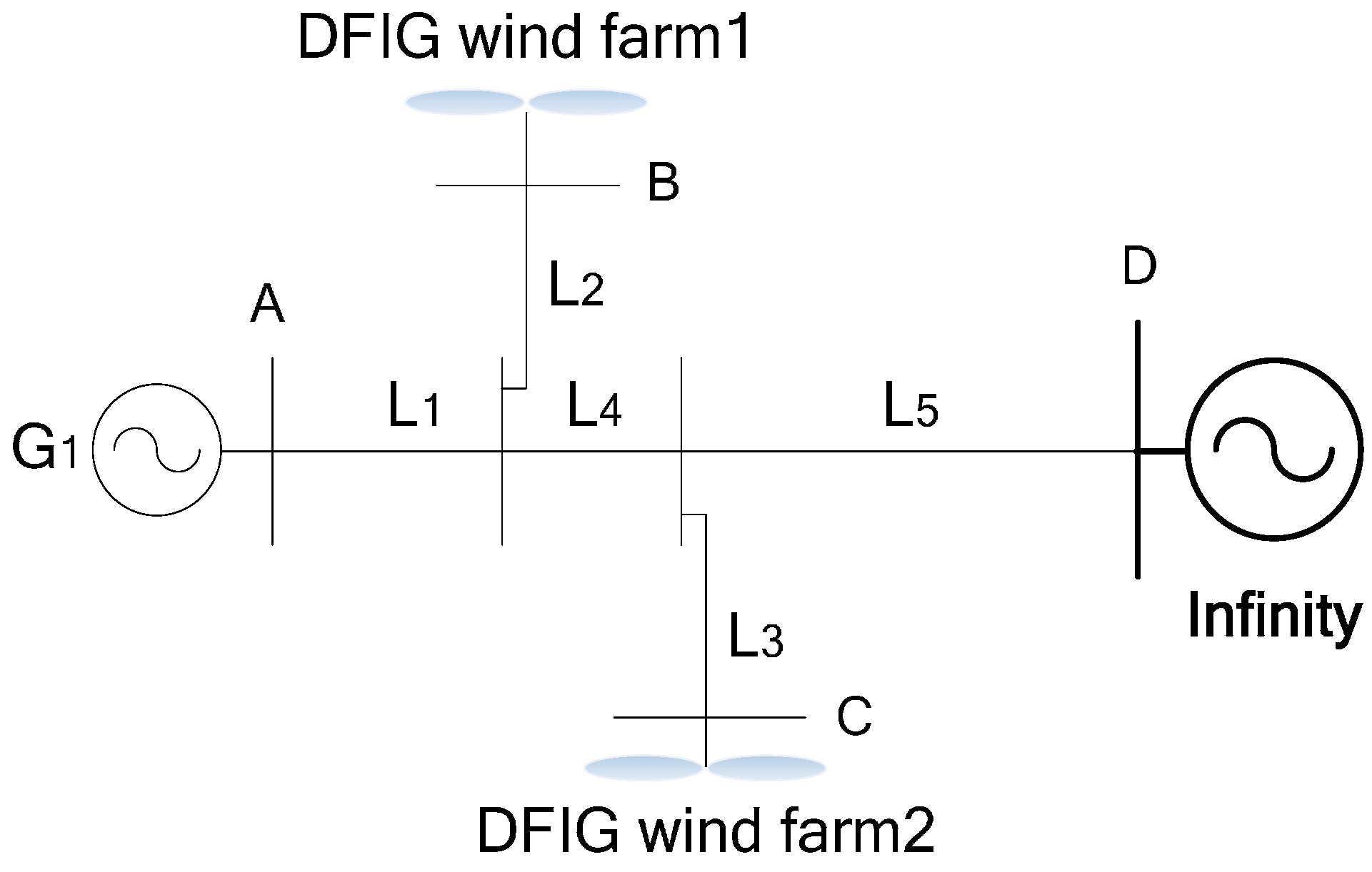
5.1. Calculation of Small-signal Stability Region Boundary of the Power System

This paper mainly studied the impact of wind power’s fluctuations on the small-signal stability of the system. Label the active power outputs of wind farm 1 and wind farm 2 as P1, P2 respectively. Keep the active power output of the conventional generator G1 at 200 MW. By fitting the sampling points, we obtained the small-signal stability region boundary as shown in Equation (17).
1.17489P1 + P2 = 456.6134
Figure 5 shows the comparison between sampling points and the fitting boundary, where P1 is the abscissa and P2 is the ordinate. According to Figure 5, they have good consistency. Details of the sampling points and errors are shown in Appendix B.
Figure 5. The contrast figure of stability region boundary.
Sustainability 07 04582 g005

5.2. Analysis of Small-signal Stability Probability of the Power System Considering the Uncertainty of Wind Power

5.2.1. Calculation of the One-step TransitionMatrix

Take the historical three years’ (2004–2006) wind speed data of two wind farms (Label the wind farms as A and B, the longitude and latitude of which are (−103.66, 45.89), (−96.74, 43.17), respectively in South Dakota, U.S.A. as the statistical object. The time interval of the data is 10 min. The wind speed data is from the American National Renewable Energy Laboratory [32]. In the two wind farms, the probabilities that wind speed exceeds 25 m/s are both less than 0.05%, which is not included within the scope of this paper. When dividing the wind speed states, the more number of states are, the more accurate the results will be. However, the amount of calculation increases accordingly. This paper divided the wind speed of a single wind farm into 11 states according to the operating condition of the wind turbine.The detail is as following: 1: [0,3); 2: [3,4); 3: [4,5); 4: [5,6); 5: [6,7); 6: [7,8); 7: [8,9); 8: [9,10);9: [10,11); 10: [11,12); 11: [12,25).
For wind speed states 1 and 11, no matter how much the wind speed changes in the intervals, the output of wind farms will not change. As for states 2 to 10, wind speed can be assumed to approximately obey the average distribution in the intervals. In this paper, the wind speeds of wind farm 1 and wind farm 2 were represented by the wind speed data of wind farm A and B. Then the total number of states was 11 × 11 = 121 after combining the states of the two wind farms. The one-step transition matrix followed the format of 121 × 121. Through data statistics, we calculated the signal-step transition matrix, details of which are in the data file “appendix-data.xlsx”.

5.2.2. Analysis of the Influence of Wind Speed’s Initial States

To study the influence of the initial states of wind farm on small-signal stability probability on short time scales, we used the one-step transition matrix and considered the case that the initial state was stable (similar to the state of interval M in Figure 2). The instability probability of each state at the next moment, namely after 10 min, are shown in Figure 6.
In Figure 6, the coordinates X, Y, and Z respectively represent the wind speed state of wind farm 1, wind speed state of wind farm 2 and the instability probability of the system. The greater the wind speed of the initial state, the larger the output of the wind farm and the system gets closer to the boundary. As can be seen from Figure 6, on short time scales, the instability probability of the system has a strong correlation with the current state. When the initial state is far from the boundary, the probability that the system loses stability in the next moment (after 10 min) is very small, which is essentially 0. While with the increase of wind speed the initial state of the system is closer to the boundary of the stability region boundary, the instability probability of the system at the next moment is greater. The maximum value of the instability probability is 8.64%.
Figure 6. The instability probability graph of each state after 10 min.
Sustainability 07 04582 g006

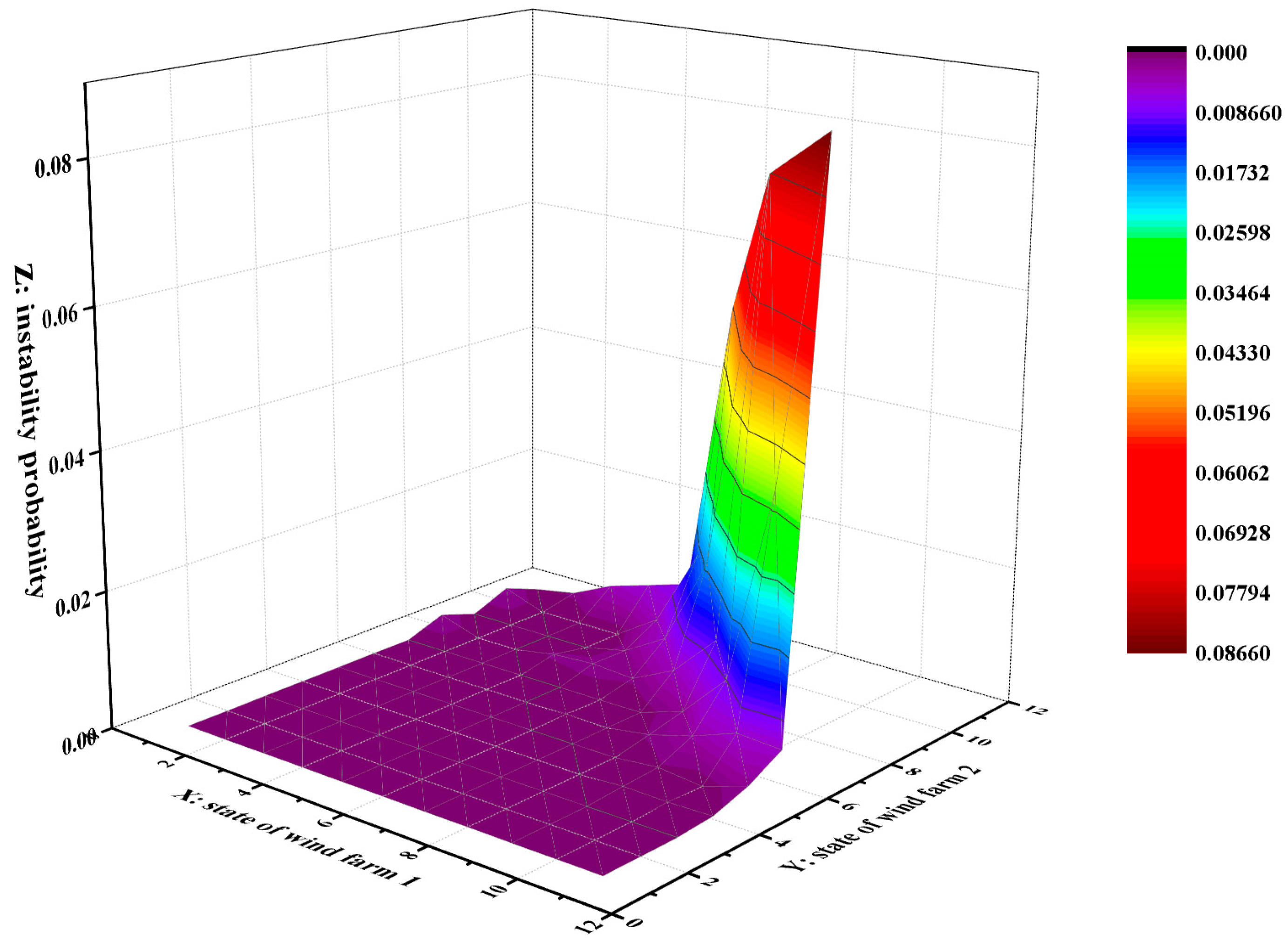
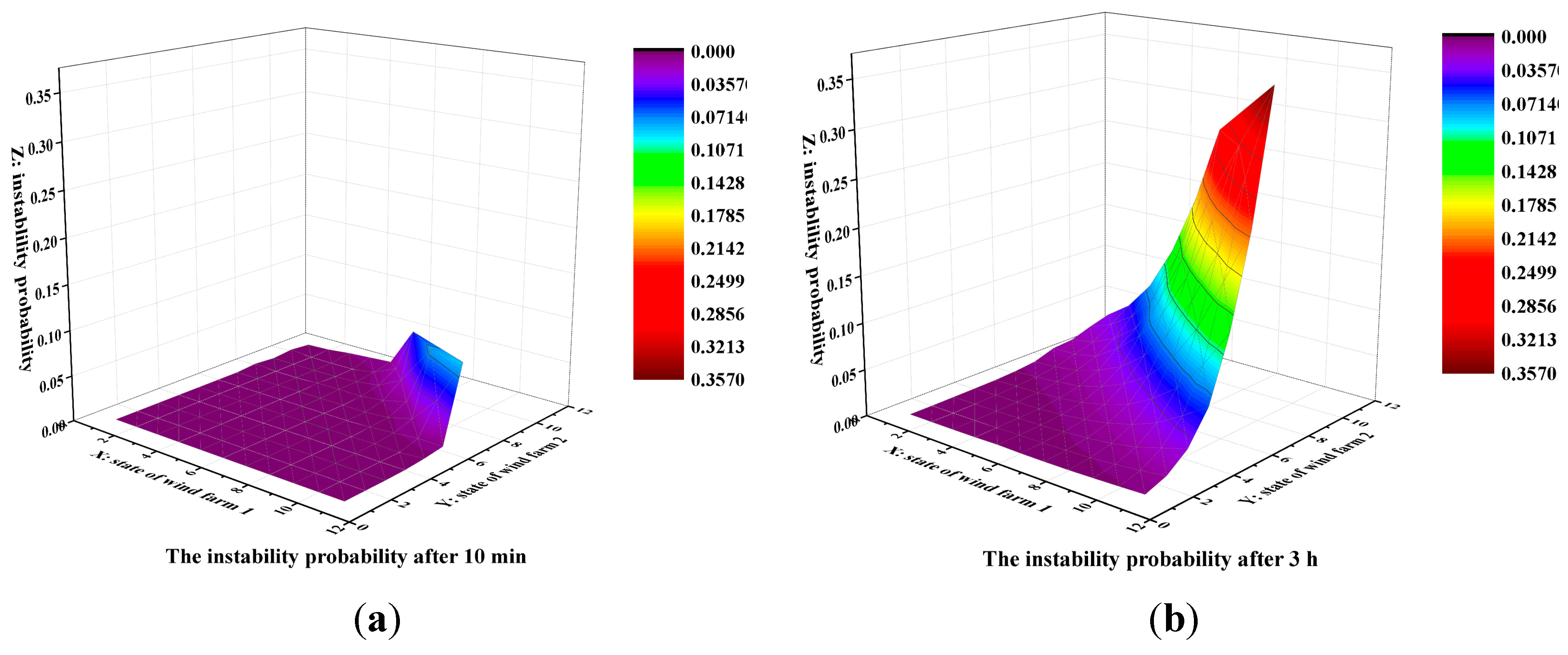
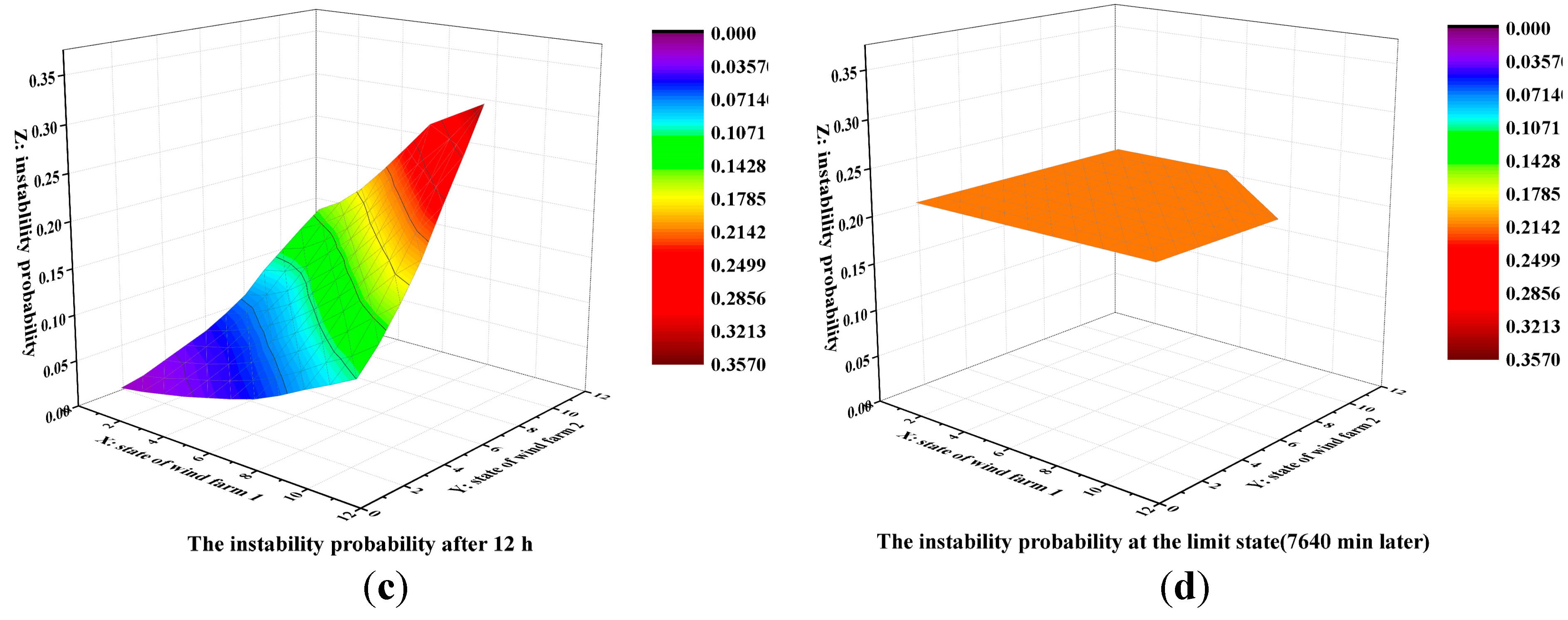
5.2.3. The Influence of Multi-time Periods

To study the change of the instability probability of each initial state in different time periods, this paper calculated the instability probabilities of each initial state after 10 min, 3 h, 12 h and the limit state (after 7640 min), respectively. The contrast is shown in Figure 7.
As can be seen from Figure 7, in the case that the initial state is far from the stability region boundary, the probability that the system loses stability gradually increases with the increase of the period of time. While in the case that the initial state is close to the stability region boundary, the probability that the system loses stability first increases quickly and gradually decreases afterwards with the increase of the period of time. Finally, when the system reaches the limit state (after 7640 minutes), no matter what the initial state is, the instability probabilities of the system are exactly the same, each of which is 21.38%.
Figure 7. The instability probability graph of each state in multi-time periods.
Sustainability 07 04582 g007aSustainability 07 04582 g007b

5.2.4. Discussion on the Simulation Results

Here, the study results are discussed as follows:
(1)
When the period of time reaches 7640 min, the calculated results of stability are the results of the small-signal stability probability of the system by the traditional method based on a probability distribution of wind speed. That is, in a long period of time, the frequency distribution of wind speed has certain probability characteristics, so the system has a small-signal stability probability and the probability value is independent of the initial state of the wind speed and only has a correlation with the overall probability distribution of wind speed.
(2)
Similarly, the small-signal stability probability of the system at the limit state or by the traditional method actually reflects the stability characteristics of the system on a considerable long time scale. However, on short time scales, the traditional method is not applicable to the change of the small-signal stability characteristics of the system caused by the change of wind speed.
(3)
On short time scales, the initial state of the system has great influence on the further stability characteristics. The steady operation point of the wind farm should be kept away from the small-signal stability region boundary.

6. Conclusions

The traditional small-signal stability probability of a power system with wind farms is applicable to the statistical results on long time scales. Conversely, this paper mainly focuses on analysis of the small-signal stability probability of a power system with wind farms in multi-time periods, especially on short time scales. Through the analysis, the conclusions are as follows:
(1)
On short time scales, the instability probability of the system has strong correlation with the current state. When the initial state is far from the boundary, the probability that the system loses stability at the next moment is very small. While when the initial state of the system is closer to the boundary of the stability region boundary, the instability probability of the system at the next moment is greater.
(2)
In the case that the initial state is far from the stability region boundary, the probability that the system loses stability gradually increases with the increase of the period of time. While in the case that the initial state is close to the stability region boundary, the probability that the system loses stability first increases quickly and gradually decreases afterwards with the increase of the period of time. Finally, when the system reaches the limit state, no matter what the initial state is, the instability probabilities of the system will be exactly the same.
(3)
When the system reaches the limit state, the calculated stability probability is independent of the initial state, which is also the result of the small-signal stability probability of the system by the traditional method based on probability distribution of wind speed, which reflects the probability characteristics of the system on a considerable long time scale.
(4)
On short time scales, the initial state of the system has great influence on the further stability characteristics. The steady operation point of the wind farm should be kept away from the small-signal stability region boundary of the system.
The study results of this paper provide a new method and support for analyzing the small-signal stability probability of power system with wind farms.

Acknowledgments

This work is supported by the project “Research of the Impact Mechanism on Self-organized Critical State by Large-scale Cluster Grid-Connected Wind Power and Identification”, funded by the National Science Foundation of China (51377053), and the project “Research on Key Techniques of Load-Net-Source Coordinated Control Based on Large-Scale Wind, Solar Power and High-Energy Load Integration”, funded by National Science and Technology Support Project of China (SQ2015BA0502239).

Author Contributions

Rundong Ge contributed to design, analysis, and the writing of this paper. Wenying Liu contributed to direction of the research and consultation. Huiyong Li made some suggestions and translated this article from Chinese to English. Jianzong Zhuo contributed to the experiment. Weizhou Wang made some suggestions. All co-authors contributed to the writing of the final research article.

Appendix

This article has two appendixes: Appendix A, Appendix A.

Appendix A

Appendix A1 DFIG Parameters

The parameters of DFIG are as follows: Pn(MW): 2; Us(V): 690; Rs(p.u.): 0.01; Xs(p.u.): 0.1; Xm(p.u.): 3.5; Rr(p.u.): 0.01; Xr(p.u.): 0.1; Hw(s): 4.02; Hg(s): 0.47; K(p.u.): 80.27.
In these parameters, the voltage and power reference values are this machine’s rated voltage and capacity.

Appendix A2 Generator Parameters

The parameters of Generator G1are as follows: Capacity (WVA) : 300; Voltage (KV): 18; xd(p.u.): 1.72; x d ( p.u. ) : 1.66; xq(p.u.): 0.23; x q ( p.u. ) : 0.378; T d 0 ( s ) : 0.8; T q 0 ( s ) : 0.12.
In these parameters, the voltage and power reference values are this machine’s rated voltage and capacity.

Appendix A3 Excitation parameters

Details of the excitation system model refer to the A-type exciter in Appendix D of reference [33]. The specific parameters are as follows: τR: 0.001; τA1: 0.05; KA: 400; τA2:0.01; VRmax:3; VRmin: -3; τE: 0.95; KE: 0.17; KF: 0.04; τF: 1; E1: 3.66; Se1: 0.03; E2: 4.89; Se2: 0.1.

Appendix A4 Line parameters

Line type is LGJ-400, L1 of 50 km in length, L2 of 10 km in length, L3 of 30 km in length, L4 of 30 km in length and L5 of 80 km in length.

Appendix B

In order to accurately express the error between sampling points and the fitting boundary, define the error σ as follows:
σ = d P 1 2 + P 2 2
where d is the distance from sampling points to the fitting boundary. After calculation, we ascertained that the average error was 0.156% and the biggest was 0.295%, which achieved a good accuracy and showed that the model was reasonable and feasible. Detailed sampling points and their error are shown in Table A1.
Table A1. The sampling points of small-signal stability region boundary and their errors.
P1(MW)P2(MW)Real partImaginary partError (%)
210208.540.000046.969830.295
200221.3206.9580730.069
190233.830.000036.933810.096
180246.030.000066.9027870.191
170257.8706.8728420.207
160269.390.000046.8413040.157
150280.680.000026.6980430.061
140291.690.000036.7501840.088
132.263000.000036.7137190.242

Conflicts of Interest

The authors declare no conflict of interest.

References

  1. Baños, R.; Manzano-Agugliaro, F.; Montoya, F.G.; Gil, C.; Alcayde, A.; Gómez, J. Optimization methods applied to renewable and sustainable energy: A review. Renew. Sustain. Energy Rev. 2011, 15, 1753–1766. [Google Scholar] [CrossRef]
  2. Hernandez-Escobedo, Q.; Saldana-Flores, R.; Rodriguez-García, E.R.; Manzano-Agugliaro, F. Wind energy resource in Northern Mexico. Renew. Sustain. Energy Rev. 2014, 32, 890–914. [Google Scholar] [CrossRef]
  3. Montoya, F.G.; Manzano-Agugliaro, F.; López-Márquez, S.; Hernández-Escobedo, Q.; Gil, C. Wind turbine selection for wind farm layout using multi-objective evolutionary algorithms. Expert Syst. Appl. 2014, 41, 6585–6595. [Google Scholar] [CrossRef]
  4. Liu, W.Y.; Ge, R.D.; Li, H.Y.; Ge, J.B. Impact of Large-Scale Wind Power Integration on Small Signal Stability Based on Stability Region Boundary. Sustainability 2014, 6, 7921–7944. [Google Scholar] [CrossRef]
  5. Slootweg, J.G.; Kling, W.L. The impact of large scale wind power generation on power system oscillations. Electr. Power Syst. Res. 2003, 67, 9–20. [Google Scholar] [CrossRef]
  6. Gautam, D.; Vittal, V.; Harbour, T. Impact of Increased Penetration of DFIG-based Wind Turbine Generators on Transient and Small Signal Stability of Power Systems. IEEE Trans. Power Syst. 2009, 24, 1426–1434. [Google Scholar] [CrossRef]
  7. Rueda, J.L.; Colome, D.G. Probabilistic performance indexes for small signal stability enhancement in weak wind-hydro-thermal power systems. IET Gener. Transm. Distrib. 2009, 3, 733–747. [Google Scholar] [CrossRef]
  8. Rueda, J.L.; Erlich, I. Impacts of Large Scale Integration of Wind Power on Power System Small-signal Stability. In Proceedings of the 4th International Conference on Electric Utility Deregulation and Restructuring and Power Technologies (DRPT), Weihai, Shandong, China, 6–9 July 2011.
  9. Bu, S.Q.; Du, W.; Wang, H.F.; Chen, Z.; Xiao, L.Y.; Li, H.F. Probabilistic analysis of small-signal stability of large-scale power systems as affected by penetration of wind generation. IEEE Trans. Power Syst. 2012, 27, 762–770. [Google Scholar] [CrossRef]
  10. Soleimanpour, N.; Mohammadi, M. Probabilistic small signal stability analysis considering wind energy. In Proceedings of the 2nd Iranian Conference on Smart Grids (ICSG), Tehran, Iran, 23–24 May 2012.
  11. Yue, H.; Li, G.Y.; Zhou, M. A Probabilistic Approach to Small Signal Stability Analysis of Power Systems with Correlated Wind Sources. J. Electr. Eng. Technol. 2013, 8, 1605–1614. [Google Scholar] [CrossRef]
  12. Carta, J.A.; Ramírezb, P.; Velázquez, S. A review of wind speed probability distributions used in wind energy analysis: Case studies in the Canary Islands. Renew. Sustain. Energy Rev. 2009, 13, 933–955. [Google Scholar] [CrossRef]
  13. Halilcevic, S.S.; Gubina, F.; Gubina, A.F. Prediction of power system security levels. IEEE Trans. Power Syst. 2009, 24, 368–377. [Google Scholar] [CrossRef]
  14. Li, J.; Wei, W. Probabilistic evaluation of available power of a renewable generation system consisting of wind turbines and storage batteries: A Markov chain method. J. Renew Sustain. Energy 2014, 6, 130–139. [Google Scholar]
  15. Wang, J.M.; Kang, J.J.; Sun, Y.F.; Liu, D.M. Load forecasting based on GM-Markov chain model. In Proceedings of the Second Pacific-Asia Conference on Circuits, Communications and System (PACCS 2010), Beijing, China, 1–2 August 2010.
  16. Li, Y.Z.; Niu, J.C.; Ru, L.; Yue, Y.T. Research of multi-power structure optimization for grid-connected photovoltaic system based on Markov decision-making model. In Proceedings of the International Conference on Electrical Machines and Systems, Wuhan, China, 17–20 October; 2008. [Google Scholar]
  17. Lawler, G.P. Introduction to Stochastic Processes, 2nd ed.; Chapman & Hall: New York, NY, USA, 1995; pp. 7–49. [Google Scholar]
  18. Michael, M.; Eli, U. Probability and Computing: Randomized Algorithms and Probabilistic Analysis; Cambridge University Press: London, UK, 2005; pp. 153–182. [Google Scholar]
  19. Shamshad, A.; Bawadi, M.A.; Wan Hussin, W.M.A.; Majid, T.A.; Sanusi, S.A.M. First and second order Markov chain models for synthetic generation of wind speed time series. Energy 2005, 30, 693–708. [Google Scholar] [CrossRef]
  20. Castro Sayas, F.; Allan, R.N. Generation availability assessment of wind farms. IEE Proc. Gener. Transm. Distrib. 1996, 143, 507–518. [Google Scholar] [CrossRef]
  21. Nicola, B.N.; Ole, H.; Birgitte, B.; Poul, S. Model of a synthetic wind speed time series generator. Wind Energy 2008, 11, 193–209. [Google Scholar] [CrossRef]
  22. Hocaoglu, F.O.; Gerek, O.N.; Kurban, M. The effect of markov chain state size for synthetic wind speed generation. In Proceedings of the 10th International Conference on Probabilistic Methods Applied to Power Systems (PMAPS 2008), Rincon, Puerto Rico, 25–29 May 2008.
  23. Yu, D.Y.; Han, X.H.; Liang, J.; Song, S.G. Study on the Profiling of China’s Regional Wind Power Fluctuation Using GEOS-5 Data Assimilation System of National Aeronautics and Space Administration of America. Autom. Electr. Power Syst. 2011, 35, 77–81. (In Chinese) [Google Scholar]
  24. Canizares, C.A.; Mithulananthan, N.; Milano, F. Linear Performance Indices to Predict Oscillatory Stability Problems in Power Systems. IEEE Trans. Power Syst. 2004, 19, 1104–1114. [Google Scholar] [CrossRef]
  25. Abed, E.H.; Varaiya, P.P.; Milano, F. Nonlinear Oscillations in Power Systems. Int. J. Elec. Power 1984, 6, 37–43. [Google Scholar] [CrossRef]
  26. Sun, Q.; Yu, Y.X. Hyper-Plane Approximation of Boundary of Small Signal Stability Region and Its Application. J. Tianjin Univ. 2008, 41, 647–652. (In Chinese) [Google Scholar]
  27. Yu, Y.X. Review of study on methodology of security regions of power system. J. Tianjin Univ. 2008, 41, 635–646. (In Chinese) [Google Scholar]
  28. Liu, W.Y.; Ge, R.D.; Lv, Q.C.; Li, H.Y.; Ge, J.B. Research on Small Signal Stability Region Boundary Model of the Interconnected Power System with Large-scale Wind Power. Energies 2015, 8, 2312–2316. [Google Scholar] [CrossRef]
  29. Fernández, L.M.; Jurado, F.; Saenz, J.R. Aggregated Dynamic Model for Wind Farms with Doubly Fed Induction Generator Wind Turbines. Renew. Energy 2008, 33, 129–140. [Google Scholar] [CrossRef]
  30. Ali, M.; Ilie, I.S.; Milanovic, J.V. Wind farm model aggregation using probabilistic clustering. IEEE Trans. Power Syst. 2008, 28, 309–316. [Google Scholar] [CrossRef]
  31. Hansen, A.D.; Jauch, C.; Sørensen, P.; Cutululis, N.; Jauch, C.; Blaabjerg, F. Dynamic Wind Turbine Models in Power System Simulation Tool DIgSILENT; The Risø National Laboratory: Roskilde, Denmark, 2003; pp. 1–82. [Google Scholar]
  32. National Renewable Energy Laboratory (NERL). Wind integration datasets. Available online: http://www.nrel.gov/wind/integratioiidatasets/ (accessed on 20 January 2014).
  33. Anderson, P.M.; Fouad, A.A. Power System Control and Stability, 2nd ed.; Wiley: West Sussex, UK, 2002; pp. 555–582. [Google Scholar]

