Detection and Modeling of Vegetation Phenology Spatiotemporal Characteristics in the Middle Part of the Huai River Region in China

Abstract

Vegetation plays an important role in atmospheric, hydrologic and biochemical cycles and is an important indicator of the impact of climate and human factors on the environment. In this paper, a method, which combines the empirical orthogonal function (EOF) and temporal unmixing analysis (TUA) methods, is applied to monitor the phenological characteristcs and spatial distribution of vegetation phenology in the middle part of the Huai River region. Based on the variance and EOF curves, the EOF provides the number of phenology modes, information which is the basis for an accurate temporal unmixing model. The TUA describes the temporal vegetation phenological details and spatial distribution. Importantly, this approach does not require assumptions, prior information or pre-defined thresholds. The vegetation phenology curves derived from the MODIS EVI data using the combined EOF and TUA methods display much more detail than the curves from Landsat TM using spectral mixture analysis (SMA). Additionally, the vegetation phenology spatial distribution from MODIS EVI is consistent with the field survey data. The combination method of EOF and TUA can be used to monitor vegetation phenology spatiotemporal change in a large area from time series of MODIS EVI data.

1. Introduction

Vegetation phenology dynamics influence the ecosystem through seasonal changes in albedo [1], canopy conductance [2,3] and by exerting strong effects on water and heat fluxes [4], carbon cycling [5] and net ecosystem productivity [6]. Therefore, accurate and detailed spatiotemporal vegetation phenology is critical to model climatic, hydrological and ecological processes [7].

Vegetation phenology has been studied using field surveys of bud, flowering and leaf-fall dates [8]. Phenology can be monitored on regional, national and global scales using remote sensing data [9,10]. Thresholds technology [11], spectral analysis [12], largest increase identification [13] and temporal unmixing analysis [14] are among the most common methods used to study vegetation phenology. However, the most important problem is to extract accurate and effective information from image time series with fewer limitations and assumptions. The combination method of empirical orthogonal function (EOF) and temporal unmixing analysis (TUA) was first provided in [15]. Based on EOF variances and EOF curves, three phenology endmembers have been used effectively to model the phenology in the Ganges-Brahmaputra delta. In this study, the combination method of EOF and TUA are used to study the phenological phenomena in the middle part of Huai River region in China, and four phenology endmembers are selected.

Phenology dimensions by EOF method could be considered the base information for temporal unmixing modelling. Phenology dimensions mean the number of phenology modes that can be distinguished from image time series through time. Dimensions could provide a way to show different image processes, to determine what processes can and cannot be distinguished. In meteorology and oceanography, the EOF and principal comment (PC) are always related to important spatiotemporal patterns. They produce statistically uncorrelated modes, but do not guarantee physical significance. Based on variances and EOF curves, EOFs provide prior statistical dimensions for a temporal unmixing model. Temporal unmixing analysis provides partial interpretation for EOF. The challenge for temporal unmixing models is to determine the number of phenology endmembers, and the statistical EOF results provide base information for modelling [15].

This paper’s objectives are: (1) to apply the combined method of EOF and TUA to produce the temporal phenology endmembers and spatial vegetation abundance in the middle part of Huai River region from MODIS EVI time series; and (2) validate the EOF and TUA methods by comparing their results with those derived from Landsat TM using spectral unmixing and with a field survey spatial map. In this study, the EOF method provide a statistical way to representing the number of phenological dimensions by variances. The temporal EOFs and corresponding spatial PCs display spatiotemporal phenological dimensions of images. Based on the base information of EOFs, the TUA method is used to extract phenological curves and unmix the spatial distribution as processes. When EOF and TUA methods are used together, they make up for each other’s shortcomings. The EOF provides the number of phenological dimensions as prior for temporal unmxing modelling. The TUA method helps to explain realistic meaning of the statistic EOFs. The spatiotemporal processes were validated using phenology curves extracted from Landsat and a phenology spatial map derived from field surveys. For estimating vegetation, MODIS EVI performs better than NDVI and is less susceptible to bias with high temporal resolution [16,17,18]. Landsat TM and ETM+ at 30-m resolution also have been used to identify vegetation phenology [19,20]. Spectral mixture analysis (SMA) could be used to map urban land cover and provide vegetation fraction that could be compared to other measures of vegetation cover [7,21]. In this study, spectral mixture analysis (Substrate-Vegetation-Dark endmembers) has been used to extract vegetation abundance time series curves that are compared with phenological endmembers from EVI, to calibrate the phenology patterns [7,22]. Finally, spatial vegetation phenology maps based on field survey [23,24,25] are compared with vegetation phenology map derived from the EOF and TUA methods.

2. Study Sites and Data

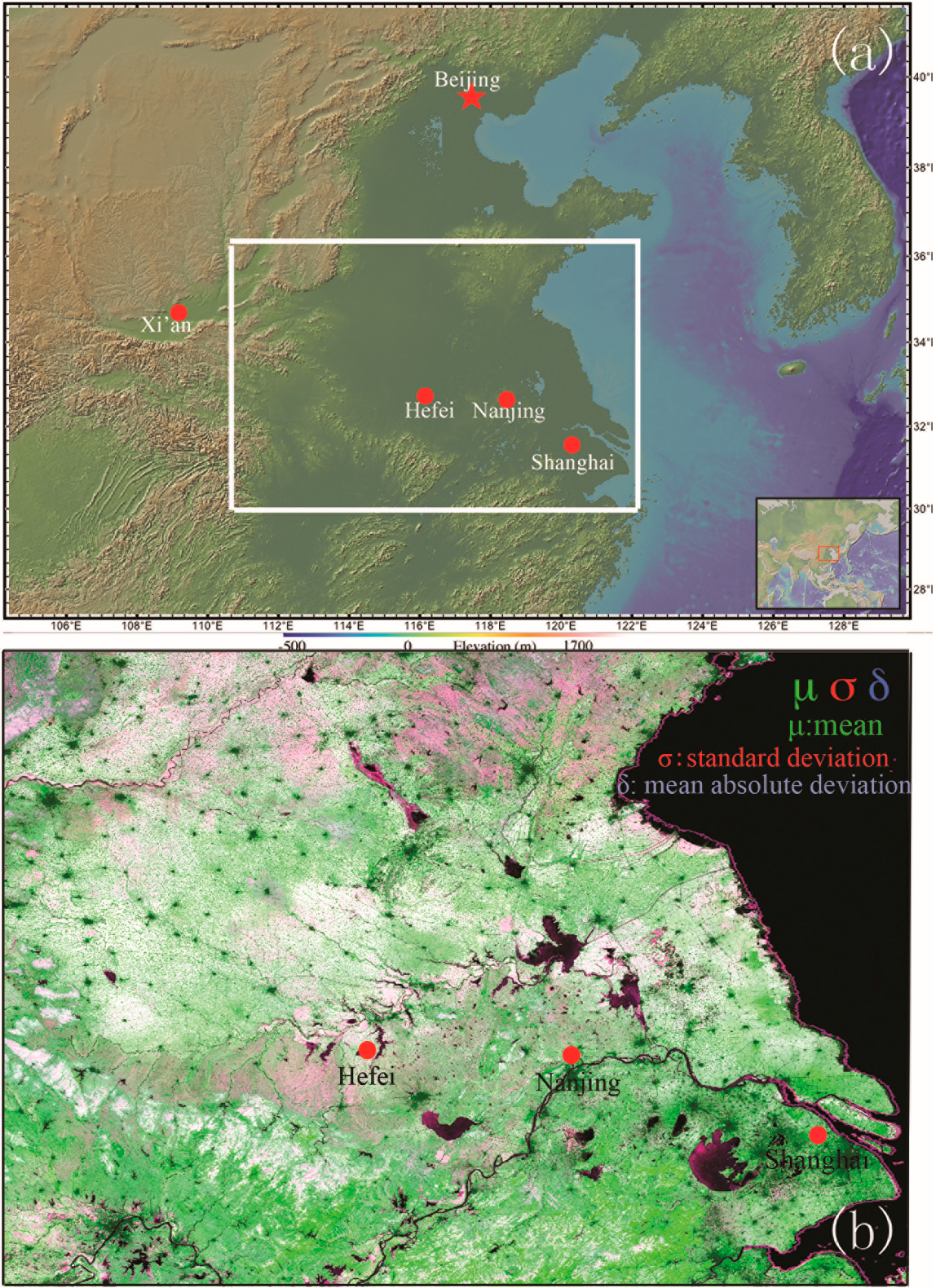
2.1. Study Sites

The study area in the middle part of the Huai River basin is located at 113°1′24″~122°0′29″E, 30°0′29″~36°2′24″N (Figure 1a). The study area covers the entire Jiangsu province and Shanghai, and part of the provinces as follows: Anhui province, Zhejiang province, Shandong province, Henan province, Hubei province, Jiangxi province, Shanxi province and Hebei province. The elevation of study area ranges from −126–1750 m. The average annual temperature is 13 °C. The average annual precipitation is 888 mm [26]. The Huai River lies between the Yangtze River and the Yellow River [27]. It marks the approximate boundary for the northern and southern climate regions in China. Its northern region is in the warm temperate zone, and its southern region is in the subtropical zone. The Huai River also bounds the subhumid and humid regions [28]. Because of these natural conditions, the study area has a diverse phenology.

The Huai River region is defined by provincial administrative boundaries and includes the entire Henan, Anhui, Jiangsu, Shanghai and Shandong provinces. In this research, however, the study area is the middle part of Huai River region because much attention has been paid to the vegetation phenology in the natural range of the Huai River region.

The temporal composite is composed of the standard deviation EVI, mean EVI and mean absolute deviation EVI (Figure 1b). The standard deviation and mean absolute deviation show the EVI value change amplitude [16]. The magenta part corresponds to high standard deviation and high mean absolute deviation. The reason for the magenta region lies in either significant vegetation change or cloud contamination. The white part corresponds to high standard deviation, high mean absolute deviation and high mean EVI. The green part shows the vegetation distribution with low vegetation change. The temporal composite shows the vegetation spatial distribution and EVI temporal change.

2.2. Data

The MODIS-EVI (Q1) 250m from February 2000 to December 2012 and Landsat data 30 m were downloaded from the USGS [29]. There are 277 scenes in the MODIS EVI dataset. There are 15 good quality Landsat images, including 11 scenes from 2003 and four scenes from 2002. The elevation data were downloaded from GeoMap. The Chinese vegetation data set at a scale of 1:1,000,000 was provided by Environmental and Ecological Science Data Center for West China, National Natural Science Foundation of China [25].

Figure 1. (a) Location and elevation map of the study area. (Based on data from Geomap); (b) Temporal moment composite of MODIS EVI (Enhanced Vegetation Index) 2000–2012. The spatiotemporal variability of vegetation is shown by the temporal mean (μ), standard deviation (σ) and mean absolute deviation (δ).2.3. Methods.

Figure 1. (a) Location and elevation map of the study area. (Based on data from Geomap); (b) Temporal moment composite of MODIS EVI (Enhanced Vegetation Index) 2000–2012. The spatiotemporal variability of vegetation is shown by the temporal mean (μ), standard deviation (σ) and mean absolute deviation (δ).2.3. Methods.

2.3. Methods

2.3.1. Empirical Orthogonal Function

Mathematically, the EOF method breaks down the original data into products of temporal and spatial functions [30,31]. The EOFs are the eigenvectors of the covariance matrix from the principle transform of the original data and represent temporal patterns. The principal components (PCs) represent the major spatial distribution of corresponding phenological patterns (EOFs). According to the EOF phenological curves characters, the corresponding spatial PCs is the basis to form the two dimensional scatter diagram for endmember selection by the TUA method below. The EOFs are statistical results and any physical meaning cannot be guaranteed. A physical process may include many statistical EOFs and many processes contribute to one statistical EOF. Recombining EOFs could produce phenological curves with physical meaning. The two dimensional scatter diagram of PCs is a basis to select phenologic endmembers and it also offers a process to recombine EOFs.

Moreover, the EOF method aims to reduce the dimensionality with a minimal loss of information, while maintaining the majority of the essential features [32,33]. The previous EOFs can represent the characters of the data because they account for the major part of the variance. In this study, according the variance and EOF curves, the EOFs could provide prior information to determine the number of phenology dimensions.

2.3.2. Temporal Unmixing Analysis

The temporal unmixing model is the extended concept from spectral mixture analysis [34]. The notion of a temporal unmixing model is that each pixel is the linear combination of different temporal endmembers and corresponding fractions [35]. The temporal endmembers can show distinct time series processes. From a mathematical perspective, the temporal unmixing model can be described as:

$${\text{DN}}_{\text{X}}={\text{E}}_1{\text{f}}_1+{\text{E}}_2{\text{f}}_2+\dots +{\text{E}}_{\mathrm{T}}{\text{f}}_{\mathrm{T}}+\text{ε}$$

DN means the digital number for each pixel. X represents each pixel position. E means temporal end members. T represents the temporal dimension, $\text{ε}$ means residual. $\text{f}$ represents the abundance of the corresponding temporal end member.

The fractions of the end members are commonly a response to:

$${\displaystyle \sum }_{\text{i}=1}^{\text{T}}{\text{f}}_{\mathrm{i}}=1{\text{f}}_{\mathrm{i}}\ge 0$$

Accurate endmembers and temporal dimensions are the key to temporal mixture models. Endmembers are in the extreme position of the feature space and represent different fundamental processes.

In a temporal unmixing model, each pixel is the linear combination of different temporal endmembers and corresponding fractions [35,36]. In this paper, the pixel purity index (PPI) is an adjunct method to TUA and makes the PC results more accurate. In the feature space, the furthest points away from the origin of coordinates must be the endmembers [37]. The PPI method involves randomly generating vectors among the feature space and recording the distance of pixels from vectors. The frequency of points with the furthest distance is the pure pixel index. The larger the pure pixel index is, the greater the possibly that the points are endmembers. The advantage of PPI is that it can distinguish extreme distance and find pure pixels. This is different from other research in which PPI is used to select endmembers. First, the dimensionality and noise reduction is performed by the PC transform. Secondly, the PPI method could keep the record of extreme distance when the original data are projected onto the random generation vectors among the dataset [38]. As a result, the PC transformation and PPI mask can keep pure pixels that represent significant phenology types. These pure pixels are extracted as temporal phenology endmembers.

2.3.3. Combining Empirical Orthogonal Function and Temporal Unmixing Analysis

Phenology endmember selection includes the determination of the number of endmembers and the spectral type. Based on the first inflection point of variance and EOF curves, EOFs provide the number of phenology patterns as a basis for the temporal unmixing model. The advantage of the EOF method is that the variance is based on the data rather than artificially pre-defined values or assumptions; therefore, it can reflect the basic data structure. Temporal unmixing analysis provides partial interpretation for EOF. Temporal unmixing analysis models areal phenology modes and spatial distribution.

2.3.4. Spectra Mixture Analysis

In linear spectral mixture analysis, pixels are modeled as linear mixtures of spectrally pure endmembers with estimated abundances [22,39]. Theoretically, the constraint equation specifies that the sum of the fractions should equal 1 and the unmixing process should make the RMS error small. Linear spectral mixture modeling is described in detail in [7]. The selection of substrate, vegetation and dark endmembers is consistent with this research [40]. In this study, SMA is taken as a calibration method. The phenology from MODIS EVI by EOF and TUA is compared with vegetation fraction curves from Landsat TM by SMA.

3. Results

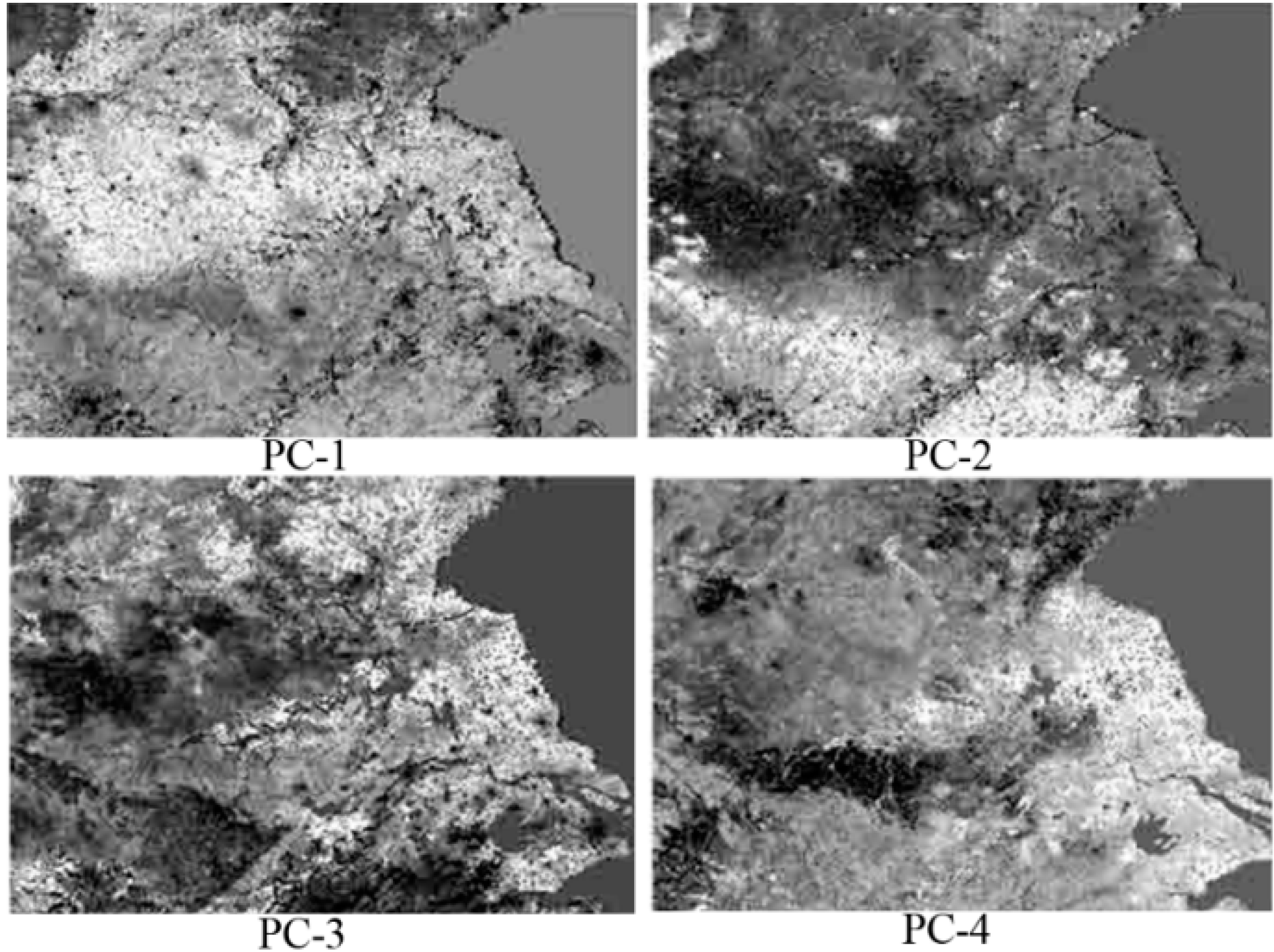
3.1. Empirical Orthogonal Function

There is an obvious inflection point at the fourth EOF (Figure 2a). The four significant EOF modes will be analyzed further; specifically, they account for 45.20%, 15.55%, 7.32% and 5.07% of the variance. The first four EOFs explain the majority of the vegetation changes in the middle Huai River region. These EOF and PC results represent vegetation changes relative to the large area. The other 273 dimensions explain the remaining 26.86% of the variance.

The EOF structure also shows that the first four have different frequency behaviors with the remaining EOFs (Figure 2c). The first four EOFs have a regular seasonal or annual frequency change that represents the main vegetation phenology changes over a large area. In contrast, the other EOFs exhibit poorly expressed annual frequency variability because the corresponding phases stem from noise or cloud contamination, or only represent phenology in small areas.

EOFs display periodicities that are related to annual, semiannual and seasonal changes (Figure 2b). The first EOF corresponding to the mean EVI has weak amplitude. The second EOF shows approximately annual cycles, and the third and fourth EOFs have regular peaks at annual and biannual periods, while these peaks identify the amplitude of the most energetic vegetation albedos in different months. In contrast, the remaining EOFs have high or low level peaks where they are linked to a small local area.

Figure 2. (a) EOFs (Empirical orthogonal function) variance of MODIS EVI dataset; (b) EOFs 1–10 for the extreme PC transform of the MODIS EVI time series; (c) Different frequency behaviors between the first four EOFs and the others.

Figure 2. (a) EOFs (Empirical orthogonal function) variance of MODIS EVI dataset; (b) EOFs 1–10 for the extreme PC transform of the MODIS EVI time series; (c) Different frequency behaviors between the first four EOFs and the others.

The light grey sections exhibit the spatial PCs that correspond to the first four temporal EOFs, which emphasize the vegetation spatial distribution in the west along the Huai River, in the south, in the north and in the east, respectively (Figure 3). Note that only the phenology mode of large spatial distribution can be identified. As a result, the EOF method provides dimensional characters to describe the spatial and temporal vegetation phenology distribution over a large area.

Figure 3. Spatial distribution of temporal EOFs 1–4 that corresponds to the area in the north along the Huai River, in the south, in the northeast and in the southeast. The variances of the first four PCs are 45.2%, 15.6%, 7.3% and 5.1%.

Figure 3. Spatial distribution of temporal EOFs 1–4 that corresponds to the area in the north along the Huai River, in the south, in the northeast and in the southeast. The variances of the first four PCs are 45.2%, 15.6%, 7.3% and 5.1%.

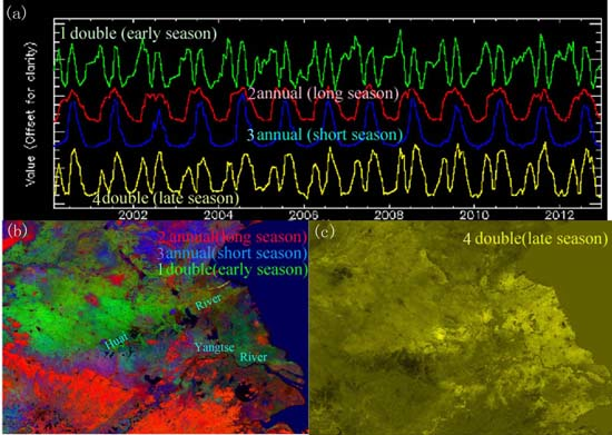
3.2. Temporal Unmixing Analysis

Based on PC transform, phenology endmembers are the vertex of a geometry that consists of two PCs as X, Y apexes (Figure 4). Taking Figure 4b as an example, it uses the PC2, PC3 defined as X, Y apexes. The three endmembers are at the extreme vertices of the pixel cloud. The fourth endmember is identified by projection in the direction of PC2 and PC4. In addition, no vegetation endmembers with low EVI are identified in Figure 4a [15]. The EOF eigenvalues describe the phenology dimensional characters, and four endmembers for the temporal unmixing model were selected in this paper.

Figure 4. Temporal feature space. The extreme vertices of the pixel cloud represent vegetation phenology endmembers. The middle parts are mixture endmembers. The topology of low order PCs also represents temporal pattern distributions as linear combinations of individual EOFs.

Figure 4. Temporal feature space. The extreme vertices of the pixel cloud represent vegetation phenology endmembers. The middle parts are mixture endmembers. The topology of low order PCs also represents temporal pattern distributions as linear combinations of individual EOFs.

The phenology endmembers are combinations of individual EOFs. The eigenvalues of the covariance explain the weight of each spatial EOF in the entire dataset. The temporal PCs express the weight of each pixel of corresponding EOFs. EOFs have statistical meaning. A spatiotemporal process may include more than one EOF and many spatiotemporal processes contribute to one EOF [15]. In the topology of pixel cloud, PCs focus on low order EOFs and combined EOFs contribute to a spatiotemporal process. The combined EOFs that represent phenology patterns exist in the geometry vertex.

A set of vegetation endmembers was selected to represent the dominant phenology mode in the middle part of the Huai River (Figure 5a). Two annual endmembers and two double cycle endmembers can be seen. There may be several days or weeks between the early season double and late season double endmembers because of climate differences caused by the ocean, elevation, sunshine and other factors. Clearly, the endmember (long season annual) has long green-up periods and a lower maximum EVI. The endmember (short season annual) has a higher maximum EVI.

The abundance map of vegetation endmembers estimated using the temporal mixture method is shown in Figure 5b,c. The figure shows that the abundance is mainly distributed over large areas corresponding to the area in the west along the Huai River, in the south, in the northeast and in the east. The annual endmember abundances are found in the south and north of the study area. The double cycle endmember abundances are distributed in the west and east of the study area along the Huai River. The total root mean square (RMS) of the temporal unmixing analysis is less than 0.02869.

Figure 5. (a) Vegetation phenological endmembers. (b, c) Fraction spatial distribution of corresponding phenological endmembers. There are four temporal endmembers: annual (short season), annual (long season), double (early season) and double (late season) for vegetation in the middle part of the Huai River region.

Figure 5. (a) Vegetation phenological endmembers. (b, c) Fraction spatial distribution of corresponding phenological endmembers. There are four temporal endmembers: annual (short season), annual (long season), double (early season) and double (late season) for vegetation in the middle part of the Huai River region.

3.3. Calibration

The base map in Figure 6a shows the substrate, vegetation and dark endmember abundances from a single RGB Landsat image from 2003 (scene ID LT 51210362003235BJC00). This study used 15 Landsat images from 2002 and 2003. Each image was unmixed using the substrate, vegetation and dark endmembers; therefore, 15 vegetation fractions were used to compose the vegetation abundance time series. According to the dots shown on the Figure 6a, the vegetation phenology temporal curve can be extracted from the vegetation abundance time series data.

Figure 6b shows the 12 vegetation phenology comparison point positions of the MODIS data, corresponding to the positions of the same color points from Landsat in Figure 6a. The base map in Figure 6b shows the abundance of the annual (long season), double (early season), and annual (short season) endmembers, corresponding to RGB. The red, green, blue and yellow dots in Figure 6b represent the position of the annual (long season), double (early season), annual (short season), and double (late season) endmembers from 23 MODIS EVI time series images from 2003.

Figure 6. (a) Base map is result of SVD mixture model for Landsat 30 m; (b) Base map is result of temporal mixture model with four periodic endmembers for MODIS 250 m. The periodic endmembers in 2003 are extracted from the MODIS and Landsat vegetation time series. The colored circles show the spatial locations of the four periodic endmembers.

Figure 6. (a) Base map is result of SVD mixture model for Landsat 30 m; (b) Base map is result of temporal mixture model with four periodic endmembers for MODIS 250 m. The periodic endmembers in 2003 are extracted from the MODIS and Landsat vegetation time series. The colored circles show the spatial locations of the four periodic endmembers.

In Figure 7, the phenology curve (color) derived from MODIS EVI data using the EOF and TUA methods is validated by comparison with the Landsat fraction curve (black). Generally, the vegetation phenology curves in 2003, as expressed by the EVI and Landsat vegetation fractions, are largely consistent, with a maximum peak at the same time and rising and falling at a similar rate. This demonstrates that the phenology endmembers selected in this study are real and characteristic.

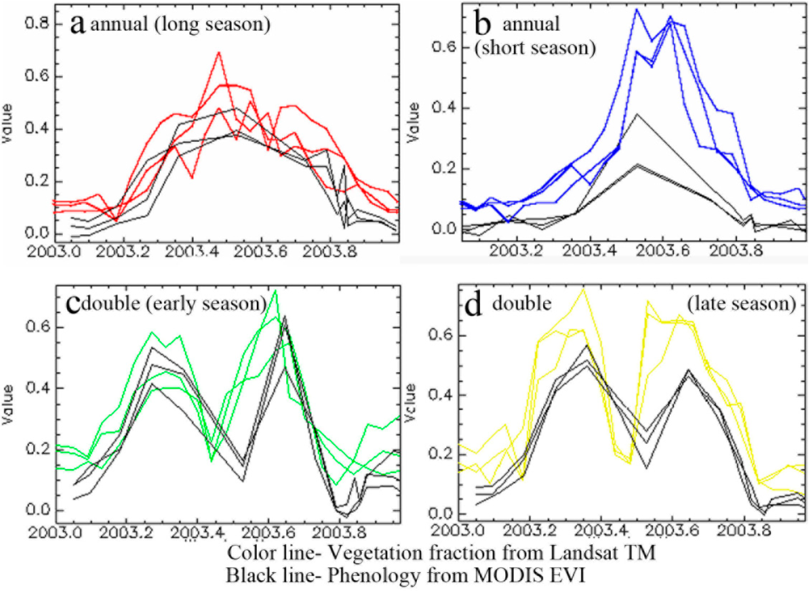
(1)

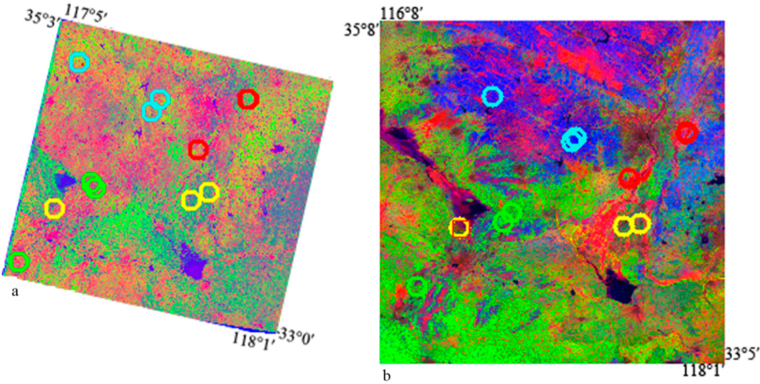
In Figure 7a, the red phenology endmembers display single peaks in May and have long temporal profiles. The phenological phase of MODIS and Landsat images agree well. The MODIS EVI describes more phenology details because there are 23 EVI images and 15 Landsat images.

(2)

In Figure 7b, the peaks of the blue phenology endmembers are both in July and the growing season is short. The peaks of Landsat fraction curves are found to maintain peaks in the same month with the EVI.

(3)

Figure 7c shows that the first peak of green endmembers is in April and the second peak is around July. The peaks of blank lines appear in the same time. These curves increase and fall at a similar rate.

(4)

In Figure 7d, the first peak of yellow phenology endmembers is in May and the second peak is in July. The peaks of blank lines are also in May and July. These curves have the same phenology phase.

The comparisons between EVI endmembers and vegetation fraction from Landsat TM aim to contrast the phenology phase, not the value. Phenology phase reflects the phenology patterns. The value of vegetation endmembers is enhanced vegetation index from MODIS. The value of vegetation fraction is the vegetation abundance by spectral mixture analysis from Landsat TM.

Figure 7. Periodic endmembers for a subset of the EVI temporal feature space. The colored periodic endmembers are extracted from the Landsat images. The black periodic endmembers are captured from MODIS EVI. These endmembers describe phenological amplitude and phase variations.

Figure 7. Periodic endmembers for a subset of the EVI temporal feature space. The colored periodic endmembers are extracted from the Landsat images. The black periodic endmembers are captured from MODIS EVI. These endmembers describe phenological amplitude and phase variations.

The advantage of MODIS EVI data is that it can be used to make temporal profiles, but the spatial resolution is 250 m, 500 m and 1000 m. Conversely, Landsat data have high spatial resolution but are often contaminated by clouds. Twenty-three EVI scenes from 2003 are compared with 15 Landsat scenes. Because of cloud cover, 10 Landsat scenes were obtained from 2003 and five from 2002. The disadvantage is that Landsat images are easily contaminated by clouds and are not sufficient temporal profiles. Single year Landsat images often cannot describe details of temporal phenology. The advantage of Landsat data is that the combination of Landsat data from several years by spectral mixture analysis can demonstrate the phenology cycles. This can also offer a way to represent phenological characteristics. In this paper, the combination of Landsat data in 2002 and 2003 is used to extract phenology curves compared with MODIS EVI in 2003 by EOF and TUA method.

4. Discussions

4.1. Comparison with Field Survey Data

Figure 5 and Figure 8a show that the spatial distribution of vegetation phenology from MODIS EVI is basically consistent with the field survey data except for a small area of forests. Note the cultivated vegetation and forest areas in Figure 8a. The distribution of annual and double vegetation in Figure 5 separately corresponds to the forest and cultivated areas in Figure 8a. The comparison also shows that the forest area in Figure 8a is larger than the area of annual vegetation in Figure 5a. The main reason is the difference in time between Figure 5, which spans from 2000–2012, and Figure 8a, which spans from 19810–2001. The spatial distribution of cropland in 2000 is undated in [24], which is consistent with the cropland distribution in Figure 5. The vegetation phenology map could be updated using the EOF and TUA methods. Compared with the field survey data, there are two crop phenology endmembers and two forest phenology endmembers.

The spatial distribution of vegetation phenology described in Figure 8b contains five types of vegetation phases from the field survey. The two-year three ripe grain fields (green) and one-year two ripe grain fields (yellow) in Figure 8b correspond well to cultivated vegetation with double early season (green) and double late season (yellow) in Figure 5. The one-year two ripe fields or three ripe parts in Figure 8b are not in accordance with the corresponding field in Figure 5 because the phenology classification is not precise in Figure 8b. Phenology based on remote sensing mainly represents total vegetation changes over large areas, and it is different from traditional remote sensing in observing the start and end dates of a single plant at a fixed point. When the ground greenness reaches a certain limit, the satellite sensors begin to extract the beginning and end date in large-scale regions. The growing season determined by remote sensing describes the active state of entire vegetation communities.

Figure 8. (a) Spatial distribution of vegetation in the middle part of the Huai River region. Notice the spatial distribution of cultivated vegetation and forests; (b) Spatial distribution of cultivated vegetation phenology. The cultivated vegetation area is divided into five phenological subspaces. Compare the phenological distribution from the temporal mixture model results and the cultivated vegetation phenology figure.

Figure 8. (a) Spatial distribution of vegetation in the middle part of the Huai River region. Notice the spatial distribution of cultivated vegetation and forests; (b) Spatial distribution of cultivated vegetation phenology. The cultivated vegetation area is divided into five phenological subspaces. Compare the phenological distribution from the temporal mixture model results and the cultivated vegetation phenology figure.

4.2. Strengths and Uncertainties

The EOF method provides the number of phenology dimensions as a basis for the TUA method, and in this lies the strength of the combined method. The most similar comparison is temporal unmixing using independent component analysis in [35]. The approach in [35] decomposes mixed observations by a remote sensor into individual crop signals in three regions covering parts of Kansas and Nebraska in the US and a third region in northwestern Turkey. The method in [35] may be appropriate for regions where the phenology patterns are known previously. Sometimes, the phenology phenomenon in certain areas is diverse (once a year, twice a year and so on), but the phenology endmember types are not known. Information on more general endmember characteristics is needed. The EOF method discussed in this paper is used to describe the dimensionality based on the dataset itself and provide the number of phenology patterns. The combined EOF and TUA methods are appropriate for areas where phenology patterns are without prior information for phenology patterns.

The number of endmembers is uncertain because it depends on the phenological characteristics of the study area. However, the EOF method described here could characterize phenology as a priori. The combined EOF and TUA method provided by Small [15] uses three phenology endmembers to describe the phenology pattern in the Ganges-Brahmaputra delta. The three phenology endmembers represent 81% of the spatiotemporal variance in the data. In this study, four phenology endmembers are selected to characterize the phenology in the Huai River region. The first four endmembers explain 73.14% of the variance corresponding to spatiotemporal processes. The first inflection point is at the fourth EOF. More phenology endmembers could be selected to describe abundant phenological spatiotemporal processes, but it is easy to overfit if the endmembers are not sufficiently independent. The EOF method provides a statistical dimensional representation. Areal phenology diversity determines the first inflection point of EOF variances, and further determines the number of dominant phenology dimensions.

4.3. Further Application

The EOF method decomposes the vegetation indexes into different directions, and these eigenvectors have clear physical meanings. In Figure 2, the fifth EOF shows a significantly decreasing trend. By comparing the fifth EOF with its corresponding spatial distribution, there is a high vegetation reduction, so the EOF eigenvectors can be used to detect the most sudden decreases in vegetation in a region. Because the balance between population, resources and environmental pollution has been neglected, there are problems such as population explosion and vegetation deterioration. The EOF method could also help detect changes to vegetation within evolving urban areas.

The vegetation phenology distribution map could be applied at large scales in China. The EOF provides phenology dimensions based on the data without assumptions, and the TUA extracts phenology endmembers that describe phenology stages at large scales. To expand the use of this method in China, the correlation between vegetation indexes and elevation must be considered. Elevation and temperature are the dominant factors that control vegetation phenology [41]. Elevation could complicate the study of regional phenology. If the combined EOF and TUA methods are applied to vegetation phenology in China, the phenology in alpine regions, such as the Tibetan Plateau, can be analyzed further.

The phenology partition could be utilized as the basis of agricultural production estimation sampling [16]. Because global warming, water shortages and extreme weather greatly impact agriculture, food security issues have gained global attention. Accurate knowledge of agricultural production and effective food security alarm forecasts could benefit agricultural trade, macroeconomic policy-making and other socioeconomic functions. Usually, sampling for agricultural production estimation is based on random statistical selection, but phenology partitions derived from the joint application of the EOF and TUA methods could narrow the sampling frame and optimize the sampling results.

5. Conclusions

The variances and EOF curves help to determine the number of phenology dimensions. A large amount of data is concentrated by the EOF method. The first inflection point appears at the fourth EOF and the first four EOF curves have regular patterns. The first four EOFs can simultaneously represent the phenology modes. The EOFs provide the number of phenology dimensions as a basis for the temporal unmixng model. The first four PCs simultaneously represent the spatial distribution of corresponding EOFs.

Phenology endmember abundance by TUA method is based on the endmembers’ extraction. The endmembers are extracted using a scatterplot based on PCs that are optimized by the PPI mask. Based on the EOF prior information, four phenology endmembers (annual long season, annual short season, double early season, double late season) are applied into a temporal unmixing model. The spatial distribution of four endmembers (short season annual, long season annual, early season double, late season double) are separately located in the north, south, west and east of the middle part of Huai river region.

By comparison, the phenology curves derived by linear spectral unmixing using Landsat fraction temporal profiles have simultaneous peaks with the EVI phenology endmembers, and both increase and fall at a similar rate. These results demonstrate that the phenology phase of endmembers and vegetation fraction are consistent. In addition, the Landsat images could be used for phenology, but it is difficult to acquire sufficient temporal profiles that are not contaminated by clouds. In this work, the phenology endmembers derived by the EOF and TUA methods can describe many more details of vegetation phenology than the Landsat images processed with spectral unmixing.

References

- Bala, G.; Caldeira, K.; Wickett, M.; Phillips, T.J.; Lobell, D.B.; Delire, C.; Marin, A. Combined climate and carbon-cycle effects of large-scale deforestation. Proc. Natl. Acad. Sci. USA 2007, 104, 6550–6555. [Google Scholar] [CrossRef] [PubMed]
- Blanken, P.D.; Black, T.A. The canopy conductance of a boreal aspen forest, Prince Albert National Park, Canada. Hydrol. Process. 2004, 18, 1561–1578. [Google Scholar] [CrossRef]
- Richardson, A.D.; Keenan, T.F.; Migliavacca, M.; Ryu, Y.; Sonnentag, O.; Toomey, M. Climate change, phenology, and phenological control of vegetation feedbacks to the climate system. Agric. For. Meteorol. 2013, 169, 156–173. [Google Scholar] [CrossRef]
- Richardson, A.D.; Black, T.A.; Ciais, P.; Delbart, N.; Friedl, M.A.; Gobron, N.; Hollinger, D.Y.; Kutsch, W.L.; Longdoz, B.; Luyssaert, S.; et al. Influence of spring and autumn phenological transitions on forest ecosystem productivity. Philos. Trans. R. Soc. Lond. Ser. B Biol. Sci. 2010, 365, 3227–3246. [Google Scholar] [CrossRef]
- Garrity, S.R.; Bohrer, G.; Maurer, K.D.; Mueller, K.L.; Vogel, C.S.; Curtis, P.S. A comparison of multiple phenology data sources for estimating seasonal transitions in deciduous forest carbon exchange. Agric. For. Meteorol. 2011, 151, 1741–1752. [Google Scholar] [CrossRef]
- Dragoni, D.; Schmid, H.P.; Wayson, C.A.; Potter, H.; Grimmond, C.S.B.; Randolph, J.C. Evidence of increased net ecosystem productivity associated with a longer vegetated season in a deciduous forest in south-central Indiana, USA. Glob. Chang. Biol. 2011, 17, 886–897. [Google Scholar] [CrossRef]
- Small, C.; Lu, J.W.T. Estimation and vicarious validation of urban vegetation abundance by spectral mixture analysis. Remote Sens. Environ. 2006, 100, 441–456. [Google Scholar] [CrossRef]
- Williams, R.J.; Myers, B.A.; Muller, W.J.; Duff, G.A.; Eamus, D. Leaf phenology of woody species in a north Australian tropocal savanna. Ecology 1997, 78, 2542–2558. [Google Scholar] [CrossRef]
- Tucker, C.J.; Elgin, J.H., Jr.; McMurtrey, J.E., III; Fan, C.J. Monitoring corn and soybean crop development with hand-held radiometer spectral data. Remote Sens. Environ. 1979, 8, 237–248. [Google Scholar] [CrossRef]
- Beck, P.S.A.; Atzberger, C.; Høgda, K.A.; Johansen, B.; Skidmore, A.K. Improved monitoring of vegetation dynamics at very high latitudes: A new method using MODIS NDVI. Remote Sens. Environ. 2006, 100, 321–334. [Google Scholar] [CrossRef]
- Studer, S.; Stockli, R.; Appenzeller, C.; Vidale, P.L. A comparative study of satellite and ground-based phenology. Int. J. Biometeorol. 2007, 51, 405–414. [Google Scholar] [CrossRef] [PubMed]
- Moody, A.; Johnson, D.M. Land-Surface Phenologies from AVHRR Using the Discrete Fourier Transform. Remote Sens. Environ. 2001, 75, 305–323. [Google Scholar] [CrossRef]
- Schwartz, M.D.; Reed, B.C.; White, M.A. Assessing satellite-derived start-of-season measures in the conterminous USA. Int. J. Climatol. 2002, 22, 1793–1805. [Google Scholar] [CrossRef]
- Lobell, D.B.; Asner, G.P. Cropland distributions from temporal unmixing of MODIS data. Remote Sens. Environ. 2004, 93, 412–422. [Google Scholar] [CrossRef]
- Small, C. Spatiotemporal dimensionality and Time-Space characterization of multitemporal imagery. Remote Sens. Environ. 2012, 124, 793–809. [Google Scholar] [CrossRef]
- Pan, Y.; Li, L.; Zhang, J.; Liang, S.; Zhu, X.; Sulla-Menashe, D. Winter wheat area estimation from MODIS-EVI time series data using the Crop Proportion Phenology Index. Remote Sens. Environ. 2012, 119, 232–242. [Google Scholar] [CrossRef]
- Houborg, R.; Soegaard, H.; Boegh, E. Combining vegetation index and model inversion methods for the extraction of key vegetation biophysical parameters using Terra and Aqua MODIS reflectance data. Remote Sens. Environ. 2007, 106, 39–58. [Google Scholar] [CrossRef]
- Waring, R.H.; Coops, N.C.; Fan, W.; Nightingale, J.M. MODIS enhanced vegetation index predicts tree species richness across forested ecoregions in the contiguous U.S.A. Remote Sens. Environ. 2006, 103, 218–226. [Google Scholar] [CrossRef]
- Goetz, S.J.; Prince, S.D. Remote sensing of net primary production in boreal forest stands. Agric. For. Meteorol. 1996, 78, 149–179. [Google Scholar] [CrossRef]
- Fisher, J.I.; Mustard, J.F. Cross-scalar satellite phenology from ground, Landsat, and MODIS data. Remote Sens. Environ. 2007, 109, 261–273. [Google Scholar] [CrossRef]
- Weng, Q.; Lu, D.; Schubring, J. Estimation of land surface temperature-vegetation abundance relationship for urban heat island studies. Remote Sens. Environ. 2004, 89, 467–483. [Google Scholar] [CrossRef]
- Small, C. The Landsat ETM+ spectral mixing space. Remote Sens. Environ. 2004, 93, 1–17. [Google Scholar] [CrossRef]
- Wu, W.B.; Yang, P.; Tang, H.J.; Zhou, Q.B.; Chen, Z.X.; Shibasaki, R. Characterizing Spatial Patterns of Phenology in Cropland of China Based on Remotely Sensed Data. Agric. Sci. China 2010, 9, 101–112. [Google Scholar] [CrossRef]
- Liu, J.; Liu, M.; Tian, H.; Zhuang, D.; Zhang, Z.; Zhang, W.; Tang, X.; Deng, X. Spatial and temporal patterns of China’s cropland during 1990–2000: An analysis based on Landsat TM data. Remote Sens. Environ. 2005, 98, 442–456. [Google Scholar] [CrossRef]
- Cold and Arid Regions Environmental and Engineering Research Institute, Chinese Academy of Sciences. Available online: http://westdc.westgis.ac.cn (accessed on 1 April 2013).
- Zhang, Y.; Shao, Q.; Xia, J.; Bunn, S.E.; Zuo, Q. Changes of flow regimes and precipitation in Huai River Basin in the last half century. Hydrol. Process. 2011, 25, 246–257. [Google Scholar] [CrossRef]
- Wang, G.; Xia, J. Improvement of SWAT2000 modelling to assess the impact of dams and sluices on streamflow in the Huai River basin of China. Hydrol. Process. 2010, 24, 1455–1471. [Google Scholar] [CrossRef]
- Gao, C.; Gemmer, M.; Zeng, X.; Liu, B.; Su, B.; Wen, Y. Projected streamflow in the Huaihe River Basin (2010–2100) using artificial neural network. Stoch Environ. Res. Risk Assess. 2010, 24, 685–697. [Google Scholar] [CrossRef]
- United States Geological Survey. Available online: http://www.usgs.gov/ (accessed on 30 January 2013).
- Kim, K.Y.; Wu, Q. A Comparison Study of EOF Techniques: Analysis of Nonstationary Data with Periodic Statistics. J. Clim. 1999, 12, 185–199. [Google Scholar] [CrossRef]
- Hannachi, A.; Jolliffe, I.T.; Stephenson, D.B. Empirical orthogonal functions and related techniques in atmospheric science: A review. Int. J. Climatol. 2007, 27, 1119–1152. [Google Scholar] [CrossRef]
- Munoz, B.; Lesser, V.M.; Ramsey, F.L. Design-based empirical orthogonal function model for environmental monitoring data analysis. Environmetrics 2008, 19, 805–817. [Google Scholar] [CrossRef]
- Yu, H.L.; Chu, H.J. Understanding space–time patterns of groundwater system by empirical orthogonal functions: A case study in the Choshui River alluvial fan, Taiwan. J. Hydrol. 2010, 381, 239–247. [Google Scholar] [CrossRef]
- Horwitz, H.M.; Nalepka, R.F.; Hyde, P.D.; Morgenstern, J.P. Estimating the proportions of objects within a single resolution element of a multispectral scanner. In Proceedings of 7th International Symposium on Remote Sensing of Environment, Ann Arbor, MI, USA, 17–21 May 1971.
- Ozdogan, M. The spatial distribution of crop types from MODIS data: Temporal unmixing using Independent Component Analysis. Remote Sens. Environ. 2010, 114, 1190–1204. [Google Scholar] [CrossRef]
- Winter, M.E. Comparison of approaches for determining end-members in hyperspectral data. In Proceedings of the 2000 IEEE Aerospace Conference Proceedings, Big Sky, MT, USA, 18–25 March 2000; Volume 3, pp. 305–313.
- Bateson, A.; Curtiss, B. A method for manual endmember selection and spectral unmixing. Remote Sens. Environ. 1996, 55, 229–243. [Google Scholar] [CrossRef]
- Chang, C.I.; Wu, C.C.; Chen, H.M. Random Pixel Purity Index. IEEE Geosci. Remote Sens. Lett. 2010, 7, 324–328. [Google Scholar] [CrossRef]
- Taramelli, A.; Pasqui, M.; Barbour, J.; Kirschbaum, D.; Bottai, L.; Busillo, C.; Calastrini, F.; Guarnieri, F.; Small, C. Spatial and temporal dust source variability in northern China identified using advanced remote sensing analysis. Earth Surf. Process. Landf. 2013, 38, 793–809. [Google Scholar] [CrossRef]
- Small, C. Multiresolution Analysis of Urban Reflectance. In Proceedings of the IEEE/ISPRS Joint Workshop on Remote Sensing and Data Fusion over Urban Areas, Rome, Italy, 8–9 November 2001; 2001; pp. 15–19. [Google Scholar]
- Sun, L.; Chen, J. Influences of topography and climate on vegetation distribution over mainland China. In Proceedings of The 10th General Assembly of the European Geosciences Union (EGU 2013), Vienna, Austria, 7–12 April 2013.
© 2015 by the authors; licensee MDPI, Basel, Switzerland. This article is an open access article distributed under the terms and conditions of the Creative Commons Attribution license (http://creativecommons.org/licenses/by/4.0/).
Share and Cite
Xu, D.; Fu, M. Detection and Modeling of Vegetation Phenology Spatiotemporal Characteristics in the Middle Part of the Huai River Region in China. Sustainability 2015, 7, 2841-2857. https://doi.org/10.3390/su7032841
Xu D, Fu M. Detection and Modeling of Vegetation Phenology Spatiotemporal Characteristics in the Middle Part of the Huai River Region in China. Sustainability. 2015; 7(3):2841-2857. https://doi.org/10.3390/su7032841
Chicago/Turabian StyleXu, Di, and Meichen Fu. 2015. "Detection and Modeling of Vegetation Phenology Spatiotemporal Characteristics in the Middle Part of the Huai River Region in China" Sustainability 7, no. 3: 2841-2857. https://doi.org/10.3390/su7032841
APA StyleXu, D., & Fu, M. (2015). Detection and Modeling of Vegetation Phenology Spatiotemporal Characteristics in the Middle Part of the Huai River Region in China. Sustainability, 7(3), 2841-2857. https://doi.org/10.3390/su7032841