The Impact of Agro-Economic Factors on GHG Emissions: Evidence from European Developing and Advanced Economies

Abstract

Environmental degradation by greenhouse gas (GHG) emissions has been an important challenge of sustainable economic development and climate changes control. Industry is the major source of CO₂ emissions, whereas 84% of global anthropogenic methane and nitrous-oxide emissions emerge from agriculture. The impact of agro-economic factors on GHG emissions in European developing economies (Southeastern Europe in focus) as compared with European advanced economies has been examined in this paper. The results have confirmed the existence of significant differences in impact of these factors depending on the level of economic development. For both groups of economies, we have confirmed the Environmental Kuznets Curve (EKC) hypothesis (inverted U-shaped relationship between GDP per capita and carbon dioxide emissions), but different sectoral outputs, too. We have also established different impacts of agro emission sources. In developing economies, we have recognized livestock breeding as a predominant factor and recommended measures for reducing the emissions in this sector, following developed economies. The findings may be useful to European developing economies as a support to implementation of binding commitments emerging from the UN Framework Convention on Climate Change (UNFCCC). In the panel analysis, we have taken into consideration the non-stationarity of the series, heterogeneity of the sample, and also examined a dynamic specification.

1. Introduction

The trend of global warming caused by increased GHG emissions has been pronounced in the last several decades. Climate changes influenced by GHG emissions have caused temperature increase of up to 2 °C [1]. Emissions of CO₂ total 58.8% out of the overall GHG emissions in the world. The existing global energetic system and economic development are directly responsible for such result [2]. CO₂ emissions (metric tons per capita) in highly advanced economies total on average 12.5 and in middle-income developed ones 3.3, whereas in low-income developed economies they total 0.28 [3]. However, more recently, large developing countries also show a pronounced growth of impact on pollution, inter alia, because they have the highest concentration of world’s population, which has an increasingly emphasized need for energy consumption.

The EKC has been used in the literature to explain the connection between economic growth and GHG emissions. In advanced economies, the EKC curve mainly has the shape of an inverted letter U (EKC hypothesis). Namely, with economic growth, emissions grow to a certain extent, and then, at one moment, the start to decline, no matter that economic growth continues (when GDP per capita increases, a portion of excess income is typically allocated for environmental problems and consequently emissions decline) [4,5,6,7]. The structure of economic growth, as well as the impact of some sectors on pollution, differ from one country to the other [2]. With advanced economies in post-industrial period, the service sector has an increasing share of total GDP, and thus in total pollution level. In addition, in developing economies, the participation of agricultural sector in total GHG emissions is increasing. However, the majority of global warming still emerges from industry [8].

Agriculture contributes 10%–12% of overall global GHG emissions, where 60% relates to global N₂O, 50% to global CH₄ and less than 1% to CO₂ [9]. When including GHG emissions emerging from the forestry sector, agriculture might have a share of 17%–30% of overall global anthropogenic GHG emissions. In 2005, developing economies increased their agricultural GHG emissions by 32%, whereas advanced countries decreased their share by 12% [10]. Major sources of agricultural GHG emissions are N₂O from land (38%), CH₄ from enteric fermentation (32%), N₂O and CH₄ from biomass combustion (12%), and N₂O and CH₄ from manure management (7%). The significance of these sources differs at the regional level depending on the level of the country’s economic development.

Empiric investigations of the impact of agriculture on climate change and respective measures for reduction of the emissions are numerous [11,12,13,14,15]. Most of these investigations relate to advanced European and world economies as well as to large developing economies (i.e. India, China, and Brazil).

The principal objective of this investigation is to conduct a comparative analysis of economic and agro factors impact on GHG emissions in developing European economies with a focus on Southeastern Europe, in comparison with advanced European economies. In accordance with previously mentioned studies, we have considered as economic factors the economic growth and indicators that reflect the impact of individual sectors, specifically industrial, service and agricultural sectors. We have also tested EKC hypothesis for both groups of economies. Complementary to former investigations, in addition to economic, the analysis has also included indicators that cover the main sources of agricultural GHG emissions (including forestry). The suggestion for GHG census in developing economies (which is in preparation or in the process of realization) is to take into consideration the country-specific emissions factors [16]. For this purpose, this study will identify these factors as well as the intensity of the impact on GHG emissions. The measures for GHG emissions mitigation following the advanced economies have also been considered, aimed at more successful implementation of environmental protection strategies in these countries where it has not been fully implemented. To the best of our knowledge, the impact of agro-economic factors on GHG emission as well as the implementation of mitigation practices in European developing economies, has not been investigated yet.

The remainder of this paper is organized as follows: Section 2 is a survey of the literature. Section 3 describes data, conceptual framework and methodology. In Section 4, the results of empiric analysis have been presented. Section 5 consists of the comparative analysis and discussion of obtained results as well as recommendations for reduction of emissions in European developing economies. Concluding considerations have been given at the end.

2. Literature Review

In the existing literature, the connection between GHG emissions and economic development has already been established [4,6,17,18,19]. The analysis of this type is very complex and it depends on a number of factors, like: size of the economy, sectorial structure, development of technology, etc. Most of the investigations relate either to a specific country or to an entire geographic region. The papers focusing on a specific country have too narrow focus, whereas the ones relating to an entire region most frequently have too generalized conclusions. Thus, several authors investigate determinants CO₂ for Austria, BRIC countries and EU countries [6,20,21].

Complementary to former investigations, Al Mamun et al. considered the countries divided according to the level of their economic development (lower income, lower middle income, upper middle income, high income OECD countries and high income non-OECD countries) [2]. In addition, they have included into their consideration the share of individual sectors in GDP, in order to include the structural versatility of economies. Duro et al. show that the structure of sectors has impact on international non-equivalence of CO₂ emissions per capita [22] .

In some studies, EKC hypothesis has been confirmed [1,6,23,24]. However, there are studies that have established different dependence between economic growth and CO₂ emissions. Thus, it is established that EKC has the shape of letter N for China (the initial deterioration of environmental conditions and then economic growth causing an improvement of the environment; however, despite the efforts of environment-friendly development, environmental circumstances cannot get better continually) and the shape of letter U for Japan (these results suggest that economic growth is not the only way to improve the quality of the environment and that the resulting EKC hypothesis is inconclusive) [4]. A cubic dependence of letter N for Austria has been established [20].

Investigating the connection between good governance and CO₂, Gani also included sectorial outputs as important indicators of versatility of economies. In addition, he has established a strong support of EKC hypothesis for developing economies at the global level. However, in his considerations he has not performed geographical division of the economies, which might neglect significant factors that can influence the output variable.

In our study, we have considered European economies divided by their level of economic development and included differences emerging from their sectorial structure. Although European economies have been included in previous investigations, to our knowledge, there are no studies in which the impact of economic growth has been studied together with sectorial outputs on GHG emissions for European developing economies where the economies of Southeastern Europe are the most represented.

The investigations studying the sources of agricultural GHG emissions are numerous as well as studies on impact reduction techniques. Smith discussed the possibility of mitigation of agricultural GHG emissions for EU 27 countries and the UK [9] . He established that soil carbon sequestration in croplands has the largest potential for reduction, whereas the economic potentials are to a high extent lower. Lesschen et al. concluded that livestock breeding has a significant impact on global warming with circa 10% of the total GHG emissions in the EU 27 [15]. The largest portion of this emerges from the dairy production sector, followed by cattle-raising. Enteric fermentation (is a digestive process by which carbohydrates are broken down by microorganisms) is the main source of GHG emissions in the European livestock sector (36%), followed by N₂O soil emissions (28%). Tubiello et al. discussed the sources from agriculture, forestry and change of land use (LUCF) [13]. They established growth of the emissions from agriculture, decrease in deforestation rates and decrease in forest sinks. They conclude that the mitigation of GHG emissions intensity is evident, but should the adequate measures not be implemented, future emissions may rise up to 30% by 2050. Hirschfeld et al. analyzed the sources of agricultural GHG emissions in Germany and established that the largest rate of 16% in Germany arises from cattle farming, followed by arable farming on moorland (15%), grassland use of moorland (13%) and mineral fertilizer use (8%) [11]. In addition, 71% of agricultural GHG emission relates to animal products including animal feed, and only 29% to production of crops, excluding animal feed. They established the mitigation potentials of agricultural production in Germany and pointed out that the transformation of conventional production into the organic farming is one of major potentials, together with eating habits of consumers change. Tuomisto et al. also established that organic farming in Europe has generally lower impact on agricultural GHG emissions in comparison to conventional farming [25].

In our study, we have dealt with impact of agro-factors, which are recognized in the literature as the major sources of agricultural GHG emissions. European developing economies have been our focus (which, to the highest extent include the countries of Southeastern Europe) as they have not been the subject of separate investigations yet.

Developing economies face many challenges when constructing national inventories of greenhouse gas (GHG) emissions, such as lack of activity data, insufficient measurements for deriving country-specific emission factors, and a limited basis for estimating GHG mitigation options [26]. For European developing economies, the results of our study can be useful for the implementation of Intergovernmental Panel on Climate Change (IPCC) recommendations for GHG inventory [27]. Namely, the majority of developing economies implement the method Tier 1 (which imply the inventory of default average value of emissions factors). However, the recommendation is to use the method Tier 2 (which imply the inventory of country-specific emissions factors for the largest sources of emissions). The results of this study will contribute to identification of such sources, by estimating the intensity of some agro factors impact.

3. Data, Conceptual Framework and Methodology

3.1. Data

For panel analysis, 18 European advanced economies and 11 developing economies were used, over the period 1960–2012 for CO₂ emissions, as well as five time points (1990, 2000, 2005, 2008, and 2010) for agro emissions of other GHG (methane and nitrous-oxide). European advanced economies (based on [28] (p.148)) considered in the analysis are: Austria, Belgium, Denmark, Finland, France, Germany, Greece, Iceland, Ireland, Italy, Malta, Netherlands, Norway, Portugal, Spain, Sweden, Switzerland, and the United Kingdom. European developing economies (based on [28] (p.150)), covered by the analysis are: Albania, Bosnia and Herzegovina, Bulgaria, Croatia, Hungary, Macedonia, Montenegro, Poland, Romania, Serbia and Turkey. The data have been taken from World Development Indicators [29]. Missing data are a huge problem, especially in developing countries. Thus, the data have been prepared in a way that missing values have been replaced with average ones for the country and then normalized.

3.2. Conceptual Framework

The main research issues discussed in the paper are:

(1)

How do the agro-economic factors influence the emission of GHG in European developing economies in comparison with advanced economies?

(2)

What are the measures for GHG emissions mitigation in agriculture in European developing economies following the advanced economies?

Most anthropological GHG emissions are from emissions of carbon dioxide emitted by the combustion of fossil fuels [30,31], as well as by the agricultural emissions of methane and nitrous-oxide [10].

In accordance with this, two dependent variables have been used in the work: CO₂_pc (CO₂ per capita), including the emission of CO₂ from the combustion of fossil fuels expressed in metric tons per capita; and GHG_pc, which includes agro emissions of methane and nitrous-oxide expressed in metric tons of CO₂ equivalent per capita.

Starting from Grossman et al. [32], who were the first to test EKC for the level of urban emission until now, there have been many studies investigating the impact of economic growth on environment pollution in various countries and regions around the world [4,6,7,33]. Different sectors have different shares of economic growth and thus also in CO₂ emissions [1,2].

Consistent with these findings, in this paper, as the economic factors influencing CO₂ emissions, the following substantial variables are discussed: GDP_pc, economic growth that reflects the size of overall economy; AVA, the size of agricultural sector; IVA, the size of industrial sector; and SVA, the size of the sector of services.

Most anthropogenic emissions of GHG (the majority of which are methane and nitrous-oxide) emerge from agriculture (up to 84% of global anthropogenic emissions [10]). The largest portion of this comes from cattle-breeding, owing to the process of cattle’s digestion, storage of natural fertilizers, and farming crops for livestock (forage). The share in emissions due to artificial fertilizers and pesticides in agricultural land used for farming crops and livestock feed [11,14,15] is also significant. Forestland is an important source of primary and secondary emissions of nitrous-oxide [34]. Agricultural land use change, like draining of moist land, and the cutting down of forests and turning them into arable land or pastures, leads to increased emissions of these gases [10,13]. There is a large number of more recent papers that indicate that the growth of urban population influences the growth of CO₂ emissions [35,36]. Urban areas consume more than 66% of global energy and generate more than 70% of global GHG emission [35]. They have established that the emissions scale of CO₂ is commensurate to the size of urban population. However, there are also investigations that have established that, more recently, time urbanization does not have an impact per se, as it depends on other factors like the level of revenues, etc. [37] or showing negative influences owing to better awareness and implementation of adequate measures [38]. Rural population increasingly consumes commercial energy and has a positive impact on emissions [39].

Consistent with these findings, in this paper, as agro factors, the following substantial variables are also discussed: Fertilizer—quantity of nutrients used per unit of arable land; AgrLand—surface area of agricultural land per capita expressed in square kilometers; Forest—surface area of forest land per capita expressed in square kilometers; CropIndex—index of all crops output with the exception of forage; FoodIndex—index of all crops output that have nutritive value (also including the crops for forage); LivestIndex—index of livestock products output (meat, milk, cheese, eggs, wool, honey, etc.); and RuralPopGrow—annual rural population growth (negative value of this indicator shows the growth of urban population).

The impact of agro factors on emission of CO₂ from fossil fuels combustion emerges mainly from production of fertilizers and use of mechanization when plowing land, crop and forage harvesting, cutting forests as well as energy consumption in output of livestock products [40,41].

This is the reason why we have also considered the impact of agro factors on CO₂ emissions from fossil factors (although, as we have already mentioned, their impact is much higher on emissions of other GHG).

3.3. Method

In this paper, we have applied the analysis of panel data, which includes observations of several individuals (in our case countries) through several time periods. Panel analysis settles the problem of data unavailability for a larg number of time periods required for time series analyses. Panel analysis solves the problems that cannot be resolved by analyses of time series or individual cross-sections of data [42]. It enables researchers to have greater flexibility in modeling the differences in behaviors among the individuals through time. In addition, panel analysis is increasingly used in investigations of the impacts on GHG emissions [38,43] because, opposite to the estimate by Granger, causality among the variables estimates the character of effect and interactive impact of variables (provides for establishing the determinants of emissions). For these reasons, we have chosen the method of panel analysis for investigation of agro-economic factors impact on GHG emissions.

Basic linear regression model in panel analysis has the following form:

$$y_{it}=\alpha +x_{it}\beta +{\mu }_i+{\lambda }_t+{\epsilon }_{it}$$

(1)

where i = 1, N individual (country) index and t = 1, T time index.

In Equation (1), disturbance term has been expressed through three components: μ_i represents unobserved individual effect, λ_t represents unobserved time effect and ε_it is a random or idiosyncratic error term. Individual effects do not vary in time and they depend exclusively on observed cross-sections (for instance, surface area of land, geographic location of land, civil war—as some of the developing economies suffered civil wars during the time of observation, etc.). On the other hand, time effects enable taking into consideration some factors typical for the observed time period that are common to all countries (for example, global economic crisis, global climatic conditions, technological progress, etc.).

First of all, we have estimated the POOLING model by application of ordinary last square (OLS) method, and then random effect (RE) model by application of generalized least squares (GLS) methods. By adding the country and time fixed effects (FE), we have estimated FE model and first difference (FD) models and conducted standard tests of panel analysis [44,45,46,47,48,49,50,51,52,53]. Multicollinearity of regressors may lead to inaccurate statistical conclusions. For multicollinearity testing, we used in our work unit root from Variance Inflation Factor (VIF) [44]. A very significant issue is the danger of spurious regressions when the data (dependent variable and regressors) are non-stationary. For stationarity of variables testing, we have used two types of tests, common unit root test [54] and individual unit root tests [55,56]. With series suffering from cross-section dependence, we applied in our work cross-sectional de-meaning, thus eliminating cross dependence [54,55]. Thereafter, we have applied standard panel unit root tests on transformed series.

In the event of heteroscedasticity and series correlation, robust covariance matrix estimation according to White [44,45,57,58,59] was applied, as well as robust estimation by means of General Feasible Generalized Least Squares method (GFGLS) [44,45].

In our work, we have also estimated the dynamic panel model in order to consider the assumption that present values of emissions depend on emissions from previous periods. In dynamic panel models Equation (2), lagged values of dependent variable (not diminishing the generality, an event was presented when only the first lag of dependent variable has been included, which we used in our work) occur as endogenous regressors that are correlated with unobserved effects, which makes standard estimators inconsistent.

$$y_{it}=\rho y_{it-1}+x_{it}\beta +{\mu }_i+{\lambda }_t+{\epsilon }_{it}$$

(2)

where i = 1,...,N individual (country) index and t = 1,...,T time index.

To estimate the dynamic model, we have used Generalized Method of Moments (GMM) [45,60], which has predominantly been designed for “lower case T, capital N“ panels (several time periods and many cross-sections). In panel analysis with capital T, dynamic bias becomes statistically insignificant and FE model gives better results [60]. Applied GMM method permits regressors that are not strictly exogenous; that is, those that are correlated with past and present occurrences of errors, fixed effects, heteroscedasticity and serial correlation within the cross-sections, but not among them. Arellano et al. suggested the model to be previously differentiated in order to eliminate fixed effects and to use GMM, that is the matrix of instruments made of all exogenous variables and lagged dependant variable in level [61]. This model is known as Difference GMM. They have also suggested the test for autocorrelation in GMM model, which is especially important when the lags are used as instruments. Blundell et al. extended the model into a system consisting of an equation in first differences and equation in levels [62]. In this model, known as System GMM, the matrix of instruments has been constructed in such a manner as to include instruments in levels for equation in differences as well as the instruments in first differences for equation in levels. In the event of heteroscedasticity and autocorrelation, applied GMM method permits the use of robust covariance matrix [45,63]. Validity of model and instruments is established by means of Saragan test of over identifying restrictions which in applied GMM estimator was also implemented for the event of heteroscedasticity [60]. In addition, serial correlation in the first-differenced errors at an order higher than 1 implies that moment conditions used by estimator are not valid. Estimator at the end also gives Wald statistics for null hypothesis that all coefficients other than the constant are null.

4. Empirical Results

For panel analysis, the statistical R packages plm, sandwich and lmtest were used [45,49,57,64].

For testing the impact of agro-economic factor on CO₂ emissions, we have derived empiric model Equation (3):

ln CO₂_pc_it = α + β_1it ln Fertilizer_it + β_2it ln AgrLand_it + β_3it ln Forest_it + β_4it ln CropIndex_it + β_5it ln FoodIndex_it + β_6it ln LivestIndex_it + β_7it ln RuralPopGrow_it + β_8it ln AVA_it + β_9it ln IVA_it + β_10it ln SVA_it + β_11it ln GDP_pc_it + β_12it ln sqGDP_pc_it + μ_i + λ_t + ε_it

(3)

For testing the impact of agro factors on emission of other GHG emissions (methane and nitrous-oxide), we have derived empiric model Equation (4):

ln GHG_pc_it = α + β_1it ln Fertilizer_it + β_2it ln AgrLand_it + β_3it ln Forest_it + β_4it ln CropIndex_it + β_5it ln FoodIndex_it + β_6it ln LivestIndex_it + β_7it ln RuralPopGrow_it + β_8it ln AVA_it + β_9it ln GDP_pc_it + μ_i + λ_t + ε_it

(4)

We have estimated empirical model Equation (3) first by means of OLS for both groups of economies (advanced and developing), including the interaction terms and we have established that majority of interaction terms is significant, which indicates that there are statistically significant differences between these two groups of economies (the results of this estimate have not been presented in this paper, but they are available upon request). For this reason, we have estimated the two panels separately, panel of advanced economies and panel of developing economies.

The results of panel analysis for advanced economies (balanced panel for n = 18 economies and T = 53 years with 954 observations) have been presented in Table 1 (the results of panel tests have been presented in

Table A1. Results of panel tests for models in Table 1.

Panel Test	Model 1 †	Model 2	Model 3	Model 4
1	BP = 109.203, df = 10, p-value < 2.2e-16			BP = 190.089, df = 78, p-value = 2.4e-11
2	LM test = 583.741, df = 1, p-value < 2.2e-16
3		chisq = 526.643, df = 53, p-value < 2.2e-16	chisq = 566.282, df = 53, p-value < 2.2e-16
4	z = 18.729, p-value < 2.2e-16	z = 6.632, p-value = 3.321e-11	z = 0.518, p-value = 0.6041
5				chisq = 0.060, p-value = 0.8071
6	F = 0.554, df1 = 520, df2 = 371, p-value = 1
7	normal = 47.501, p-value < 2.2e-16
8	normal = 7.059, p-value = 1.681e-12
9	normal = 38.580, p-value < 2.2e-16
10			F = 37.653, df1 = 17, df2 = 926 p-value < 2.2e-16
11			F = −7.969, df1 = 35, df2 = 891, p-value = 1
12			F = 5.158, df1 = 52, df2 = 874, p-value < 2.2e-16
13		chisq = 6.343, df = 10, p-value = 0.786		chisq = 118.681, df = 10, p-value < 2.2e-16

^† Model 1—Pooling; Model 2—RE (random.method = “amemiya”, “twoways”); Model 3—FE (“within”, “twoways”); Model 4—FD.

).

Table 1. Determinants of CO₂ emissions from fuel combustion for advanced economies.

Variable	Model 1 †,††	Model 2	Model 3	Model 4	Model 5
Constant	−0.008	−0.250		0.011 ***	−0.010 ***
Fertilizer	0.192 .	0.086	−0.129	0.046 .	0.051 ***
AgrLand	0.051	−0.117 **	−0.118 *	0.051	0.044 ***
Forest	0.002	0.039	0.028	−0.069 *	−0.093
CropIndex	−0.090	0.022	−0.089	0.026	0.027 ***
LivestIndex	0.797 **	0.655 *	0.484 *	−0.037	−0.037 ***
RuralPopGrow	−0.114	−0.032	−0.025	0.030	0.025 ***
AVA	−0.074	0.039	0.173 **	0.063 *	0.065 ***
IVA	0.211	0.089	0.227	0.086 *	0.086 ***
SVA	0.220	−0.049	−0.021	0.039	0.043 ***
GDP_pc	−0.042	−0.115 **	−0.121 *	0.028 **	0.066 ***
sqGDP_pc					−0.031 ***
R-squared	0.418	0.315	0.259	0.044	0.960
Residual standard error (SE)	0.230	0.173	0.154	0.059	0.059

^† Model 1—Pooling—HC consistent coefficients; Model 2—RE (“two ways”)—HC consistent coefficients; Model 3—FE (“within”, “two ways”)—HC consistent coefficients; Model 4—FD—coefficients; Model 5—FD GFGLS (“within”)—coefficients; ^†† Signif. codes: 0; “***” 0.001; “**” 0.01; “*” 0.05; “.” 0.1; “ ” 1.

Table 1. Determinants of CO₂ emissions from fuel combustion for advanced economies.

Variable	Model 1 †,††	Model 2	Model 3	Model 4	Model 5
Constant	−0.008	−0.250		0.011 ***	−0.010 ***
Fertilizer	0.192 .	0.086	−0.129	0.046 .	0.051 ***
AgrLand	0.051	−0.117 **	−0.118 *	0.051	0.044 ***
Forest	0.002	0.039	0.028	−0.069 *	−0.093
CropIndex	−0.090	0.022	−0.089	0.026	0.027 ***
LivestIndex	0.797 **	0.655 *	0.484 *	−0.037	−0.037 ***
RuralPopGrow	−0.114	−0.032	−0.025	0.030	0.025 ***
AVA	−0.074	0.039	0.173 **	0.063 *	0.065 ***
IVA	0.211	0.089	0.227	0.086 *	0.086 ***
SVA	0.220	−0.049	−0.021	0.039	0.043 ***
GDP_pc	−0.042	−0.115 **	−0.121 *	0.028 **	0.066 ***
sqGDP_pc					−0.031 ***
R-squared	0.418	0.315	0.259	0.044	0.960
Residual standard error (SE)	0.230	0.173	0.154	0.059	0.059

^† Model 1—Pooling—HC consistent coefficients; Model 2—RE (“two ways”)—HC consistent coefficients; Model 3—FE (“within”, “two ways”)—HC consistent coefficients; Model 4—FD—coefficients; Model 5—FD GFGLS (“within”)—coefficients; ^†† Signif. codes: 0; “***” 0.001; “**” 0.01; “*” 0.05; “.” 0.1; “ ” 1.

The first column presents the pooled model. Owing to correlation of regressor FoodIndex with regressors LivestIndex and CropIndex, we have excluded it from the model. We have established that there is no multicollinearity for other regressors as the root from VIF for all of them is less than two (the multicollinearity of regressors test results are available upon request).

The tests of homoscedasticity and serial non-correlation have rejected the null hypothesis. For that reason, we have thus applied robust estimation to the table and they have presented HC (heteroscedasticity and series correlation) consistent coefficients. Pesaran CD test [51] rejects null hypothesis on cross-sectional (cs) independence. However, since N < T (18 < 53), correlation of cs residuals does not have an impact on consistency of model and accuracy of SE. The results of Chow test are strongly against the rejection of null hypothesis on poolability of slope coefficients.

Null hypothesis on insignificance of unobserved effects (individual, time and two ways) has been rejected on basis of Lagrange Multiplier test. On the basis of the results of this test, we have added country and time effects and estimated “two ways“ RE and FE model. The results have been presented in the second and third column. Like in pooling model, heteroscedasticity and serial correlation has been established and consequently robust estimation applied. By F test, we have established the significance of fixed country and two ways effects. Hausman test is strongly against the rejection of null hypothesis that country and time effects are random variables that are uncorrelated with regressors.

In the event of non-stationarity of regressors and dependable variable, there is a danger of spurious regression. The tests of stationarity (common and individual unit root tests) indicate that almost all series in levels are non-stationary, whereas they are stationary in first differences (the results of unit root tests have not been presented here but they are available upon request). This is why we have estimated FD model and the result has been presented in the fourth column of the Table 1 (due to heteroscedasticity, we have applied robust estimation). Wooldridge’s first-difference test confirms that FD model is better than FE; that is, the residuals in FE model follow a random walk.

Almost all of the estimated models have a low coefficient of determination (R-squared) and especially FD model. For robust estimation, we have also applied General FGLS on series in first differences (FD GFGLS). The results have been presented in the last column of the table. This model gives the best values for R-squared and RSE.

The results of panel analysis for developing economies (balanced panel for n = 11 countries and T = 53 years with 583 observations) have been presented in Table 2 (the results of panel tests have been presented in the

Table A2. Results of panel tests for models in Table 2.

Panel Test	Model1 †	Model 2	Model 3	Model 4
1	BP = 84.887, df = 10, p-value = 5.5e-14			BP = 84.887, df = 10, p-value = 5.5e-14
2	LM test = 450.575, df = 1, p-value < 2.2e-16
3		chisq = 393.969, df = 53, p-value < 2.2e-16	chisq = 386.77, df = 53, p-value < 2.2e-16
4	z = 15.115, p-value < 2.2e-16	z = 2.190, p-value = 0.02849	z = −2.528, p-value = 0.0115
5				chisq = 0.266, p-value = 0.606
6	F = 1.33, df1 = 468, df2 = 53, p-value = 0.01
7	normal = 39.987, p-value < 2.2e-16
8	normal = 4.516, p-value = 6.3e-06
9	normal = 31.468, p-value < 2.2e-16
10			F = 54.704, df1 = 10, df2 = 562, p-value < 2.2e-16
11			F = –4.482, df1 = 42, df2 = 520, p-value = 1
12			F = 8.467, df1 = 52, df2 = 510, p-value < 2.2e-16
13		chisq = 1.077, df = 10, p-value = 0.1		chisq = 138.352, df = 10, p-value < 2.2e-16

† Model 1—Pooling; Model 2—RE (random.method = “amemiya”, “twoways”); Model 3—FE (“within”, “twoways”); Model 4—FD.

).

Table 2. Determinants of CO₂ emissions from fuel combustion for developing economies.

Variable	Model 1 †, ††	Model 2	Model 3	Model 4	Model 5
Constant	0.388 **	0.028		0.006 ***	0.007 ***
Fertilizer	−0.027	0.006	0.003	0.018	0.016 ***
AgrLand	0.120	−0.006	−0.007	0.006 .	0.010 ***
Forest	0.123 **	0.221 ***	0.240 ***	−0.005	−0.094 .
CropIndex	−0.018	0.175 **	0.164 **	0.035	0.028 ***
LivestIndex	0.307 ***	−0.078 ***	−0.098 **	0.067 ***	0.041 ***
RuralPopGrow	0.203	0.088	0.085	−0.011	−0.003 ***
AVA	−0.065	0.029	0.040	−0.083	−0.084 ***
IVA	0.720 **	0.454 ***	0.438 ***	0.239 ***	0.244 ***
SVA	0.439 *	0.141	0.135	−0.098 .	−0.092 ***
GDP_pc	0.228 .	0.009	0.008	0.054 *	0.171 ***
sqGDP_pc					−0.149 ***
R-squared	0.720	0.572	0.516	0.088	0.969
Residual standard error (SE)	0.180	0.099	0.094	0.060	0.060

^† Model 1—Pooling—HC consistent coefficients; Model 2—RE (“two ways”)—HC consistent coefficients; Model 3—FE (“within”, “two ways”)—HC consistent coefficients; Model 4—FD—coefficients; Model 5—FD GFGLS (“within”)—coefficients; ^†† Signif. codes: 0; “***” 0.001; “**” 0.01; “*” 0.05; “.” 0.1; “ ” 1.

Table 2. Determinants of CO₂ emissions from fuel combustion for developing economies.

Variable	Model 1 †, ††	Model 2	Model 3	Model 4	Model 5
Constant	0.388 **	0.028		0.006 ***	0.007 ***
Fertilizer	−0.027	0.006	0.003	0.018	0.016 ***
AgrLand	0.120	−0.006	−0.007	0.006 .	0.010 ***
Forest	0.123 **	0.221 ***	0.240 ***	−0.005	−0.094 .
CropIndex	−0.018	0.175 **	0.164 **	0.035	0.028 ***
LivestIndex	0.307 ***	−0.078 ***	−0.098 **	0.067 ***	0.041 ***
RuralPopGrow	0.203	0.088	0.085	−0.011	−0.003 ***
AVA	−0.065	0.029	0.040	−0.083	−0.084 ***
IVA	0.720 **	0.454 ***	0.438 ***	0.239 ***	0.244 ***
SVA	0.439 *	0.141	0.135	−0.098 .	−0.092 ***
GDP_pc	0.228 .	0.009	0.008	0.054 *	0.171 ***
sqGDP_pc					−0.149 ***
R-squared	0.720	0.572	0.516	0.088	0.969
Residual standard error (SE)	0.180	0.099	0.094	0.060	0.060

^† Model 1—Pooling—HC consistent coefficients; Model 2—RE (“two ways”)—HC consistent coefficients; Model 3—FE (“within”, “two ways”)—HC consistent coefficients; Model 4—FD—coefficients; Model 5—FD GFGLS (“within”)—coefficients; ^†† Signif. codes: 0; “***” 0.001; “**” 0.01; “*” 0.05; “.” 0.1; “ ” 1.

Similar to the advanced economies panel, we have excluded the regressor FoodIndex because the correlation and other regressor have not shown multicollinearity. Slope coefficients are constant, on the basis of Chow test. Like the previous panel, the existence of unobserved effect, heteroscedasticity and serial correlation has been established (in accordance with this, country and time effects have been added and robust estimation HC coefficients have been applied), random model is consistent, fixed country and time effects are significant, data are non-stationary in level and stationary in first differences, FD model is more efficient than FE model and General FGLS model on the series in first differences gives the best values for R-squared and RSE.

In empirical model Equation (4), we have established statistically significant differences between the advanced and developing economies, therefore we have also considered two separate panels (the results are available upon request).

The results of panel analysis for advanced economies (balanced panel for n = 18 economies and T = 5 years with total of 90 observations) have been presented in Table 3 (the results of panel tests have been presented in

Table A3. Results of panel tests for models in Table 3.

Panel Test	Model 1 †	Model 2	Model 3	Model 4	Model 6
1	BP = 9.048, df = 8, p-value = 0.338
2	LM test = 48.144, df = 1, p-value = 3.96e-12
3		chisq = 24.224, df = 5, p-value = 0.0002	chisq = 28.272, df = 5, p-value = 3.2e-05
4		z = −1.114, p-value = 0.265	z = −0.886, p-value = 0.376
5				chisq = 2.782, p-value = 0.095
6	F = 0.87, df1 = 32, df2 = 45, p-value = 0.657
7	normal = 11.399, p-value < 2.2e-16
8	normal = −1.471, p-value = 0.141
9	normal = 7.02, p-value = 2.22e-12
10			F = 57.642, df1 = 17, df2 = 64, p-value < 2.2e-16
12			F = 1.835, df1 = 4, df2 = 60, p-value = 0.134
13		chisq = 1.377, df = 8, p-value = 0.995		chisq = 3.375, df = 8, p-value = 0.909
14					chisq(16) = 18 (p-value = 0.3239)
15					normal = −0.8241667 (p-value = 0.40984)
16					normal = −0.6338902 (p-value = 0.52615)
17					chisq(9) = 14750.19 (p-value = < 2.22e-16)

^† Model 1—Pooling; Model 2—RE (random.method = “amemiya”, “twoways”); Model 3—FE (“within”, “individual”); Model 4—FD; Model 6—SYS GMM (“ld”, “onestep”, “individual”).

).

Table 3. Determinants of agro GHG (methane and nitrous-oxide) emissions for advanced economies.

Variable	Model 1 †,††	Model 2	Model 3	Model 4	Model 5	Model 6
Constant	0.441 **	−0.161		−0.021 *	−0.025 ***
Fertilizer	0.645 **	0.181 **	0.061	0.123 .	0.096 *	0.106 .
AgrLand	0.217 ***	0.019	−0.071	0.021	0.018	0.021
Forest	0.212 **	0.167 *	0.232 .	0.163	0.176	0.048 *
CropIndex	0.413	−0.196 .	−0.271 *	−0.137	−0.036	−0.130
LivestIndex	0.019	0.183	0.158	0.144 *	0.031	0.002 .
RuralPopGrow	−0.113	−0.012	−0.009	−0.022	−0.021	−0.061
AVA	0.031	0.139 *	0.114	0.095 **	0.072 **	0.032 *
GDP_pc	0.043	−0.030	−0.049	−0.015	−0.002	−0.001
GHG_pc (-1)						0.853 ***
R-squared	0.615	0.277	0.269	0.248	0.980	0.977
Residual standard error (SE)	0.230	0.060	0.054	0.051	0.053	0.062

^† Model 1—Pooling—HC consistent coefficients; Model 2—RE (“two ways”)—HC consistent coefficients; Model 3—FE (“within”, “two ways”)—HC consistent coefficients; Model 4—FD—coefficients; Model 5—FD GFGLS (“within”)—coefficients; ^†† Signif. codes: 0; “***” 0.001; “**” 0.01; “*” 0.05; “.” 0.1; “ ” 1.

Table 3. Determinants of agro GHG (methane and nitrous-oxide) emissions for advanced economies.

Variable	Model 1 †,††	Model 2	Model 3	Model 4	Model 5	Model 6
Constant	0.441 **	−0.161		−0.021 *	−0.025 ***
Fertilizer	0.645 **	0.181 **	0.061	0.123 .	0.096 *	0.106 .
AgrLand	0.217 ***	0.019	−0.071	0.021	0.018	0.021
Forest	0.212 **	0.167 *	0.232 .	0.163	0.176	0.048 *
CropIndex	0.413	−0.196 .	−0.271 *	−0.137	−0.036	−0.130
LivestIndex	0.019	0.183	0.158	0.144 *	0.031	0.002 .
RuralPopGrow	−0.113	−0.012	−0.009	−0.022	−0.021	−0.061
AVA	0.031	0.139 *	0.114	0.095 **	0.072 **	0.032 *
GDP_pc	0.043	−0.030	−0.049	−0.015	−0.002	−0.001
GHG_pc (-1)						0.853 ***
R-squared	0.615	0.277	0.269	0.248	0.980	0.977
Residual standard error (SE)	0.230	0.060	0.054	0.051	0.053	0.062

^† Model 1—Pooling—HC consistent coefficients; Model 2—RE (“two ways”)—HC consistent coefficients; Model 3—FE (“within”, “two ways”)—HC consistent coefficients; Model 4—FD—coefficients; Model 5—FD GFGLS (“within”)—coefficients; ^†† Signif. codes: 0; “***” 0.001; “**” 0.01; “*” 0.05; “.” 0.1; “ ” 1.

Regressor FoodIndex has been excluded due to correlation in the same way as in the previous panels. On the basis of Chow test, slope coefficients are constant. Studentized Breusch–Pagan test opposes rejection of null hypothesis on homoscedasticity. However, the tests of autocorrelation of residuals and serial correlation reject the null hypothesis, thus the HC coefficients have been presented in the table. Pesaran CD test opposes rejection of null hypothesis on cs independence, therefore there is no danger of contemporaneous correlation. It has been established that there are unobserved countries and “two ways“ effects so the “two ways“—RE and “individual“—FE models (F test has established the significance of country fixed effects and insignificance of “two ways“ fixed effects) were estimated. Hausman test is against the rejection of null hypothesis on RE model consistence. Wooldridge’s first-difference test is against the rejection of null hypothesis that FD model is more efficient than FE model. Since T = 5 is a minor case, we have not treated the stationarity of series. General FGLS model on series in level gives robust estimation with determination coefficient of approximately 96%.

Finally, since N > T, we have also estimated a dynamic panel model in order to consider the possibility present emission depends on previous levels of emissions. We have applied System GMM estimator (this estimator is the preferable dynamic panel model in many applications [65]), where we used as valid instruments all exogenous variables and the first lag of the endogenous (dependent) variable, in level and in first difference (lags of higher order have no statistically significant impact). The results have been presented in the last column of Table 3. The results of Sargan test are against rejection of null hypothesis on validity of model and instruments. Zero second-order autocorrelation in the first-differenced errors implies no evidence of model misspecification. Wald test rejects null hypothesis that all coefficients other than the constant are zero.

The results of panel analysis for developing economies (balanced panel for n = 10 countries and T = 5 years with a total of 50 observations) have been presented in Table 4 (the results of panel tests have been presented in

Table A4. Results of panel tests for models in Table 4.

Panel Test	Model 1 †	Model 2	Model 4
1	BP = 3.912, df = 8, p-value = 0.865
2	LM test = 9.978, df = 1, p-value = 0.001584
3		chisq = 4.709, df = 5, p-value = 0.4525
4		z = −1.168, p-value = 0.243
6	F = 1.7, df1 = 32, df2 = 5, p-value = 0.2912
7	normal = 3.6092, p-value = 0.0003071
8	normal = −1.077, p-value = 0.281
9	normal = 1.790, p-value = 0.0734
10		F = 12.653, df1 = 9, df2 = 32, p-value = 2.84e-08
14			chisq(16) = 10 (p-value = 0.86663)
15			normal = −1.206876 (p-value = 0.22748)
16			normal = 1.280697 (p-value = 0.2003)
17			chisq(9) = 1951.815 (p-value = < 2.22e-16)

^† Model 1—Pooling; Model 2—FE (“within”, “individual”); Model 4—SYS GMM (“ld”, “onestep”, “individual”).

).

Regressor FoodIndex has been excluded owing to correlation in the same way as in the previous panels. Chow test shows that slope coefficients are constant. By the analysis it has been established that heteroscedasticity is not present. In pooling model, AR (1) (autoregressive model of order 1) errors have been detected, for which reason HC coefficients have been presented. Unobserved country effects have been confirmed and, in accordance with this, “individual“ RE and FE models estimated. Hausman test (chisq = 27.8317, df = 8, p-value = 0.0005073) has shown that RE model is inconsistent and for this reason it has not been presented in the table. In FE model, serial correlation and cs dependence have not been established. Fixed country effects are significant. FD estimator is statistically insignificant (F-statistic: 1.06477 on 8 and 31 DF, p-value: 0.41212), therefore, it has not been presented in the table. Robust estimation by General FGLS, with determination coefficient of circa 84% has been presented in the third column. Dynamic estimator has been presented in the last column. In dynamic specification, the first lag of independent variable occurs as endogenous regressor as it has been established that the lags of higher order do not have statistically significant impacts. The results of Sargan test, zero second-order autocorrelation and Wald test imply no evidence of model misspecification.

Table 4. Determinants of agro GHG (methane and nitrous-oxide) emissions for developing economies.

Variable	Model 1 †,††	Model 2	Model 3	Model 4
Constant	−0.279
Fertilizer	0.611 ***	−1.207 **	−0.686 **	0.155
AgrLand	0.244 .	−0.069	−0.050	0.002
Forest	0.154	1.265 **	0.708 .	−0.213 .
CropIndex	−0.488	−0.058	−0.024	0.049
LivestIndex	0.423 .	0.435	0.291	0.344 **
RuralPopGrow	−0.356	0.071	0.114	−0.157
AVA	−0.103	0.133 .	0.090 .	0.014 .
GDP_pc	−0.498 *	−0.135	−0.114	−0.077
GHG_pc (-1)				0.786 ***
R-squared	0.368	0.461	0.842	0.801
Residual standard error (SE)	0.393	0.184	0.197	0.231

^† Model 1—Pooling—HC consistent coefficients; Model 2—RE(“two ways”)—HC consistent coefficients; Model 3—FE (“within”, “two ways”)—HC consistent coefficients; Model 4—FD—coefficients; Model 5—FD GFGLS (“within”)—coefficients; ^†† Signif. codes: 0; “***” 0.001; “**” 0.01; “*” 0.05; “.” 0.1; “ ” 1.

Table 4. Determinants of agro GHG (methane and nitrous-oxide) emissions for developing economies.

Variable	Model 1 †,††	Model 2	Model 3	Model 4
Constant	−0.279
Fertilizer	0.611 ***	−1.207 **	−0.686 **	0.155
AgrLand	0.244 .	−0.069	−0.050	0.002
Forest	0.154	1.265 **	0.708 .	−0.213 .
CropIndex	−0.488	−0.058	−0.024	0.049
LivestIndex	0.423 .	0.435	0.291	0.344 **
RuralPopGrow	−0.356	0.071	0.114	−0.157
AVA	−0.103	0.133 .	0.090 .	0.014 .
GDP_pc	−0.498 *	−0.135	−0.114	−0.077
GHG_pc (-1)				0.786 ***
R-squared	0.368	0.461	0.842	0.801
Residual standard error (SE)	0.393	0.184	0.197	0.231

^† Model 1—Pooling—HC consistent coefficients; Model 2—RE(“two ways”)—HC consistent coefficients; Model 3—FE (“within”, “two ways”)—HC consistent coefficients; Model 4—FD—coefficients; Model 5—FD GFGLS (“within”)—coefficients; ^†† Signif. codes: 0; “***” 0.001; “**” 0.01; “*” 0.05; “.” 0.1; “ ” 1.

5. Discussion of Results

Although some European developing economies do not have quantified obligations of GHG gases reduction, as members of United Nations Framework Convention on Climate Changes (UNFCCC) they have committed themselves to submit the national report on its implementation. In the scope of the mentioned report it is necessary to make an inventory of emissions of gases with greenhouse effect, where this analysis may provide additional support.

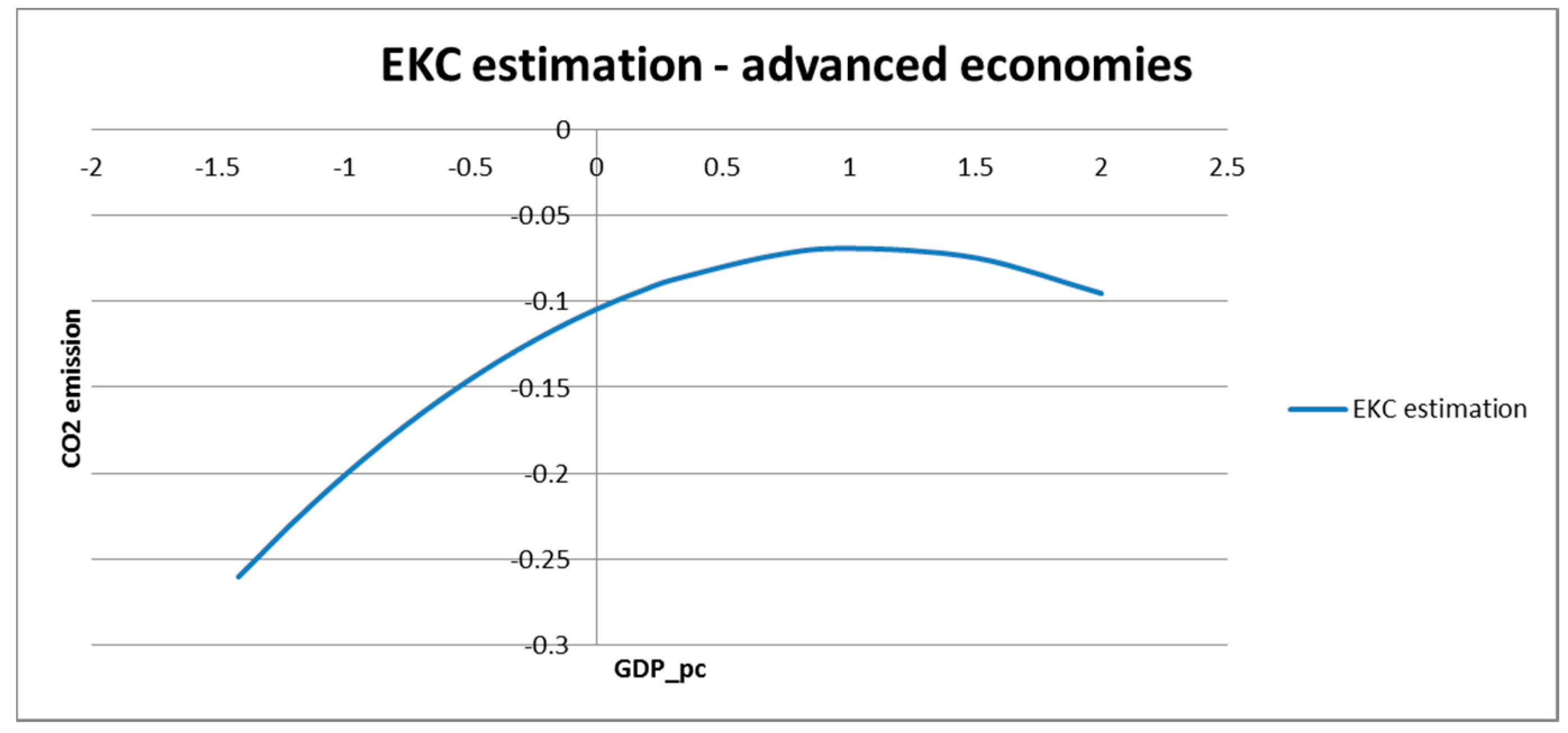
On basis of model 5 (Table 1), for advanced economies, as far as the economic factors are concerned, we have established that economic growth (GDP_pc) has a small positive impact, whereas the squared amount (sqGDP_pc) has a negative impact, which have confirmed EKC hypothesis for these countries (Figure 1). This result is consistent with the findings of Han et al. who have empirically proved the EKC hypothesis for 19 OECD countries [66], as well as with the findings of Acaravci et al., which have confirmed the EKC hypothesis for some of EU countries [6]. The results also show that in advanced European economies the impact of sectoral outputs is positive and statistically significant, which coincides with Al Mamun et al.. From model 5, we see that the impact of the industrial sector (IVA) is the largest, followed by the agricultural (AVA) and service (SVA) sectors with similar values. These results clearly suggest that the size of the industrial sector also determines to the highest extent the growth of CO₂ emissions, which coincides with [1]. Al Mamun et al. established that services sector in highly advanced world economies has an increasing share of CO₂ emissions, whereas for agriculture they have established a decreasing share owing to the application of modern technologies [2].

In addition, one can notice a positive, statistically significant impact of artificial fertilizers use on CO₂ emissions, due to combustion of fuel aimed at production, transportation and application of fertilizer. The surface area of agricultural land (AgrLand) also has a somewhat less positive impact due to the use of fuel for cultivation and adaptation, as well for as crops production (CropIndex) owing to the application of fuel for land cultivation, harvesting, etc. Livestock (LivestIndex) has a negative statistically significant impact (use of fuel in production of forage, meat, milk and other livestock products). This might be explained by the fact that other factors have much higher impacts in this model, which stresses, with high accuracy, their interdependent impact. However, Models 1–3 point to positive and statistically significant impact of livestock-breeding as an individual factor. On the basis of model 5, the size of forestland (Forest) does not have a statistically significant impact on CO₂ emissions. This finding might be explained by the fact that in advanced European economies forest cutting and their change into arable land is performed in a controlled manner. With model 4, we have a statistically significant negative impact of forest size. This might be explained by the fact that forests influence mitigation of CO₂ emissions absorption during the photosynthesis and by storing C in the biomass.

Figure 1. Estimation of EKC for advanced economies.

Figure 1. Estimation of EKC for advanced economies.

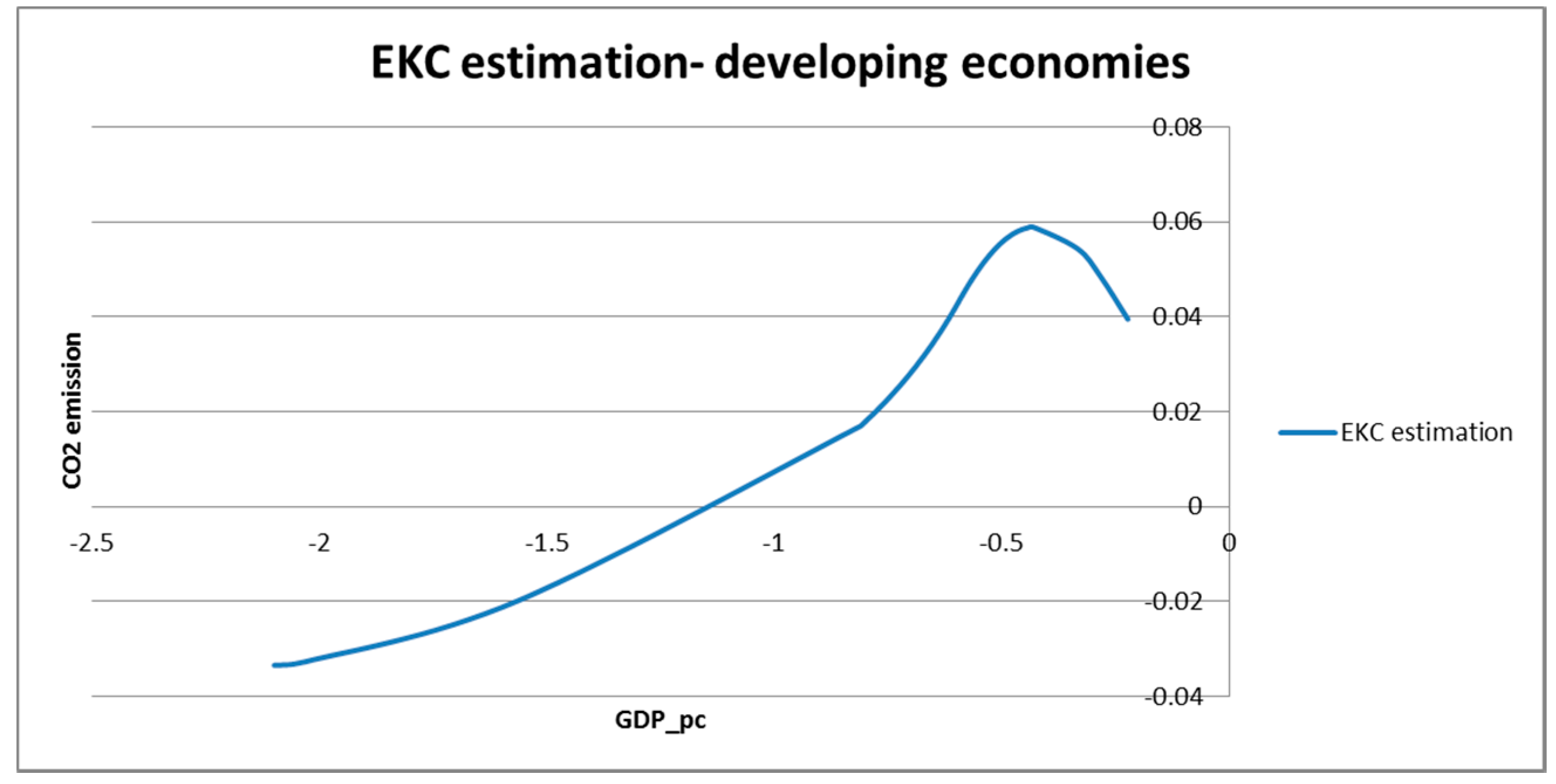
Table 2 presents the results of model estimate for European developing economies. According to model 5, growth of GDP per capita for these economies has significantly higher statistical impact on CO₂ emission compared to advanced economies. This finding shows that advanced economies have higher preferences towards environment quality. Squared economic growth (sqGDP_pc) has statistically significant negative impact, which confirms the dependence of emission on economic growth in the form of an inverted U, whereas we have also confirmed the EKC hypothesis for developing economies (Figure 2). A large number of previously mentioned studies has confirmed this hypothesis for developing economies [1,2,19].

Although, for both groups of countries, EKC has the shape of an inverted U, in developing economies EKC increases progressively unlike advanced economies where the EKC growth is slower. According to Panayotou et al., developing and developed countries find themselves on different sides of the EKC. Developing countries find themselves where the U.K. was 150 years ago, the U.S. 100 years ago, and Japan 50 years ago: when income growth, structural change, capital accumulation, and trade all contributed to rapidly growing CO₂ emissions [67]. The main reason for the rapid growth of emission in developing economies is the use of inappropriate technologies. According to Galeotti et al., considering that many developing countries are on the verge of industrialization, effective technological cooperation should be put in place to reach a sound cooperation between developed and developing countries. In the absence of such policies, governments of developing countries will pursue increases in per capita income with existing technology and this will adversely affect overall CO₂ emissions [68].

Figure 2. Estimation of EKC for developed economies.

Figure 2. Estimation of EKC for developed economies.

With sectorial outputs for developing economies, model 5 shows that industrial sector has the highest positive impact among all examined factors, whereas the services and agricultural sectors have negative impact. Opposite to advanced economies, where the sectorial output is almost on an equal footing, this finding shows that in developing economies industrial sector has a predominating impact. However, with model 1, which does not include country and time effects, it is interesting that the service sector has a positive, statistically significant impact. Growth of rural population (that is decrease of urban population) statistically makes impact on mitigation of CO₂ emissions in developing economies, which was expected. However, in advanced economies, this impact is positive, which is explained by the fact that the rural population consumes increasingly more energy owing to larger use of technology.

This finding is in harmony with [39]. On total CO₂ emissions from fuels combustion in developing economies, the second largest positive impact, after industrial sector, belongs to livestock breeding. This might be explained by the fact that modern (green) technologies in livestock breeding, fodder and livestock output, which, as a rule are used in advanced economies, are used to a lesser extent here. Use of artificial fertilizers (Fertilizer), cultivation and adaptation of agricultural land (AgrLand) and crops breeding (CropLand) have statistically significant, but lower impact on CO₂ increase as compared to livestock breeding, different form advanced economies. The reason for this is smaller scope of production and use of agro-chemical agents and technology, and thus also lower fuel consumption. Forests have statistically significant and high impact on mitigation of emitted CO₂, which shows that in these countries degradation of forests is not present and that climatic conditions are favorable for CO₂ absorption and its storage in forest soil during the process of photosynthesis.

The impact of agro-factors on CO₂ emissions mainly emerges from the use of fuel in agricultural production, as well as, to a small extent, from carbon-dioxide emissions from agricultural lands (which by its large portion is again absorbed by photosynthesis and stored in the soil by natural circulation of this gas in agro systems). Net flux of agricultural emissions of CO₂, as compared to the total emissions, is rather small.

However, agro-factors have much higher impacts on emissions of other GHG emisions (methane and nitrous-oxide). The main sources of these gases in agriculture are microbiological transformation of nitrogen from arable land and applied fertilizers as well as decomposition of organic matters in the process of livestock digestion and from stored fertilizers emission. However, forest fires also have an impact on concentration of these gases. Forests in which land cultivation is performed (agroforestry), draining and adaptation of forest and wetland into the arable land and pastures, restoration of degraded arable land, etc. also have impacts.

Table 3 features the results of model estimates for impact of agro factors on other GHG for advanced European economies. Dynamic model presented in the sixth column has the best performances, therefore we will use this model for the analysis.

According to this model, statistically significant impacts on increase of GHG (N₂O and CH₄) emissions is attributed to production and use of artificial fertilizers and forests, whereas livestock breeding has a lower impact. Surface area of agricultural land does not have a statistically significant impact, which points to the fact that in European economies land use change is performed in a controlled manner and to a lower extent.

Increased use of artificial fertilizers and its main ingredient nitrogen results in larger quantity of this ingredient in land than the crops can effectively use, and thus by emitting of this surplus in form of nitrous-oxide. Global disturbances of natural circulation of nitrogen caused by increased anthropogenic emission of this gas result in increasing decomposition of nitrogen in forest ecosystems [34]. As a result, especially acid forestland consists of larger quantities of nitrogen, which causes higher N₂O emissions. This also depends on climatic conditions, traits of land and vegetation. In Northern and Western Europe, to which most advanced economies belong, forestland is rich in carbon and has a high rate of acidity (opposite to Mediterranean and Balkan economies, where the land has lower acidity and contains a high rate of clay). This is the reason why the forests in Northern and Western European countries have impacts on increase of GHG emissions (coefficient with Forest is positive and statistically significant).

In developed countries, livestock breeding has a small positive statistically significant impact owing to implementation of adequate strategies for GHG emissions mitigation, some of them being adding dietetic additives in fodder, efficient storage of fertilizers, efficient strategies of calves fattening in more juvenile age, in order to shorten their life and thus the CH4 emissions from the process of digestion, etc.

Dynamic model 6 includes, as a regression variable, GHG emissions from the previous year. The results indicate that the quantity of these gases emitted in previous year has high and statistically significant impact, because, inter alia, the concentration of these gases increases from year to year much more than it is absorbed in natural agro systems. Accumulated quantities of anthropogenic emissions of these gases have impact on their increasingly higher emission. Atmospheric concentration of nitrous oxide approximately increases by 0.25% each year [34]. This finding on impact of accumulated emissions from previous year is a very robust finding in our work.

Models 2 and 3 show that crop production that does not include forage (CropIndex) has a negative impact on increase of GHG emissions. Forage production is included in outcome of livestock products (LivestIndex), which has positive impact on GHG emissions. Therefore, production of livestock products, including forage, has greater impact on the environment than crop production for people. Approximately 60% of arable land in Germany is used for this purpose, and only 30% for crops necessary for human nutrition [11]. This shows increased consumption of meat and dairy products in comparison with cereals and vegetables. Decreases in consumption of these products could have double benefit, in regards to both health and ecology.

The increase of rural population does not have statistically significant impact on GHG emissions. Increase of agro sector output (AVA) has statistically positive impact on increase of emissions of CH₄ and N₂O, which is in harmony with the findings in [10].

Table 4 presents the results of estimate of GHG emissions model for European developing economies.

On the basis of dynamic model 4, in European developing economies, which mainly belong to the Mediterranean and Balkans regions, forests have statistically negative impact on GHG emission, opposite to advanced European economies. This is the consequence of Mediterranean climate and properties of land that consists of a higher rate of clay and lower acidity; thus, lower quantities of nitrogen are absorbed [34]. Negative coefficient shows that the forests in this region absorb in nitrogen circulation cycle more of the nitrogen from the air than they emit. This is consistent with the findings in [34].

The impact of land area is statistically insignificant, like in advanced economies. Use of artificial fertilizers has positive, but not statistically significant impacts. Organic production generally has a positive impact on the environment because the land has higher contents of organic substances and smaller losses of nutrients [25]. However, constraints for implementation of organic agriculture in developing economies are significant, including demanding procedures, education of producers, decline of yields, level of income, etc. Model 4 shows that Livestock production (LivestIndex) has the largest positive impact on GHG emissions, opposite to advanced economies where the largest impact of use of fertilizers has been recorded (Fertilizer). This shows that in European developing economies modern technologies are insufficiently used in breeding and nutrition of livestock, storage of fertilizers and output of livestock products.

The recommendations for mitigating the emissions of GHG that emerges from the livestock production, for these economies are: combining of diary with meat production (slaughtering of older cows that do not produce quality milk any longer), instead of sole calves fattening, thus decreasing the production of forage for animals; rational use of forage (putting additives in the form of antibiotics, probiotic and vaccines that influence methane emissions mitigation in the digestion process); and efficient management of artificial fertilizer [10,25]. One of the main actuating factors for overcoming the constraints in implementation of these recommendations is the change of mind set and education of farmers as well as the financial support of agrarian policy at the state level.

Crop production for human nutrition does not have statistical impact on GHG emissions. However, in all models, a positive coefficient has been obtained (although statistically insignificant), opposite to advanced economies where there has been a negative coefficient in all models. A conclusion derived from this is that more vegetable products are consumed for nutrition in developing economies than in advanced economies.

Models 2 and 3 indicate the statistically significant negative impact of use of artificial fertilizers. This finding shows that in European developing economies artificial fertilizers are used less than the natural ones, therefore from this source the emissions of N₂O are much lower than in advanced economies.

The impact of emission level from the previous year, like in the case of advanced economies, has a very high significance threshold. This robust finding on impact of accumulated emissions from the previous year has been obtained owing to the results of dynamic model 4.

The impact of the agro sector is statistically significant and positive, as we expected, like in advanced economies and it is consistent with the fact that a high rate of total CH₄ and N₂O emissions (even up to 84%) emerges from this sector. GDP per capita growth has no statistical impact on GHG emissions in developing economies, which coincides with the finding for advanced European economies.

In general, it may be stated that there are significant differences of environmental impact depending on the level of economic development. Predominating factors of impact on GHG emissions identified for advanced economies are the use of artificial fertilizers, whereas for developing countries these are the sources from livestock breeding. Identified sources might be used for the implementation of an inventory of GHG emissions for developing economies, since they have committed themselves to UNFCCC. Namely, model results indicate country-specific factors and the intensity of its impact on GHG emissions and present an important input for the realization of the GHG inventory and mitigation strategies considered in developing countries

6. Conclusions

Emissions of GHG are the main cause of climate changes. UNFCCC has foreseen the scenario for all the countries on how to reduce emissions. According to the obligations emerging from Kyoto Protocol, countries have been divided into two groups, on the basis of their industrial development level into advanced and developing economies. Whereas the highly-industrialized countries, grouped into Annex I, have to reduce GHG emissions by 5%–10%, developing countries, including the countries of Southeastern Europe, do not have such obligation; however, they have to participate in the so-called “Program of Clean Development“. This defines their binding commitment to make a GHG emissions sources inventory.

Identification of impact of sources on GHG emissions is significant for implementation of the assumed binding commitments, especially as regulation is concerned. Opposite to advanced European and global economies and large global developing economies, in which, in the literature, this impact has been considerably studied already, there is no similar analysis for developing economies focusing on Southeastern Europe.

Thus, in this study, the impact of agro-economic factors on GHG emissions in European developing countries (especially Southeastern Europe countries) has been analyzed in comparison to advanced European economies as well as with consideration to measures for reducing GHG emissions from agriculture in these countries.

The research has been conducted by econometric panel analysis, taking into consideration non-stationarity of time series, including the effects of countries and time periods, which might have a significant impact on emissions, as well as dynamic specification, which provides for investigation of impact of emissions from previous periods. Complementary to some other methods that estimate the impact of individual independent variables on the dependent variable, this method estimates the interdependent impact of independent variables, enabling the establishment of determinants of the emissions. When estimating the parameters, the models were obtained with high coefficient of determination and small standard error, therefore; the interdependence of factors has been established with high level of accuracy. The results have shown that there are significant differences of impact on emissions depending of the level of economic development of analyzed countries.

For both groups of economies, EKC hypothesis has been confirmed as well as the strongest impact of industrial sector on CO₂ emissions, which emerge from combustion of fossil fuels. In developing economies, service and agricultural sectors do not influence the increase of CO₂ emissions, which is the opposite of advanced European economies where the impact of all three sectors is positive with relatively small differences. The finding that in advanced countries the growth of rural population has small, but positive effect on CO₂ emissions is interesting, and opposite to developing economies where this impact is negative.

For developing economies, it has been established that livestock breeding has a predominant impact on agricultural GHG emissions (methane and nitrous-oxide), as opposed to advanced economies where the use of artificial fertilizers has the largest impact. In developing economies, mainly those from the Southeastern Europe, the land area of forests has statistically negative impact on emissions of methane and nitrous-oxide, due to the characteristics of soil, which is the opposite of advanced European economies where a positive impact has been recorded. On basis of dynamic model, it has been established for both groups of countries that accumulated quantities of anthropogenic emissions of these gases influence their increasingly higher emission.

On the basis of the obtained results, recommendations of measures for reducing the impact on agro GHG emissions in livestock the breeding sector for developing economies, which has been identified as the main source, have been given. As one of the ways to reduce agro emissions, measures have been recommended for transition from conventional to organic agricultural production. Recommended measures represent a support to creators of internal agrarian policies of discussed developing economies for their implementation of binding commitments resulting from the UN Framework Convention.

Mainly the developing economies of Southeastern Europe and their comparison with advanced European economies have been the subject of interest of this investigation. Future investigations may embrace wider region which includes the remaining European countries, as well as the comparison with developing economies from the other parts of the world.