A Hybrid Stochastic Numerical Framework for Predictive Groundwater Risk Mapping: Integrating Time-Dependent Scenarios in a Strategic Alpine Aquifer

Abstract

Sustainable groundwater management represents a main goal for the future in the context of climate change and increasing anthropogenic pressure. In recent decades, intrinsic vulnerability assessment and risk mapping have been established as some of the most important tools for groundwater preservation, but they have also shown limitations due to their static nature and their failure to account for the inherent uncertainty of hydrogeological parameters. This study proposes an innovative hybrid framework that integrates traditional overlay-index methodology (SINTACS Release 5) with stochastic numerical modeling to assess groundwater contamination risk and evolve it into a dynamic time-dependent tool. This methodology was applied to a case study of the Lapisina Valley phreatic aquifer (Northeastern Italy), a strategic area for drinking water supply. Numerical simulations were implemented to reproduce groundwater flow using the MODFLOW-NWT code. To address parametric uncertainty, 237 stochastic realizations of the modeling domain were generated using the Latin Hypercube Sampling method, randomizing hydraulic conductivity values. Advective transport was simulated through forward particle tracking using the MODPATH code, starting from the identified and classified hazard sources within the study area. Assuming the absence of attenuation during transport allowed for a conservative worst-case scenario. The result was the definition of a probabilistic contaminant propagation factor, a time-dependent indicator that quantifies the probability of pollution arrival to a specific discrete portion of the domain. This probabilistic factor was combined with three indexes commonly utilized for risk assessment (the intrinsic vulnerability index, hazard index, and value of the resource) to generate four contamination risk maps representing different timestep scenarios (5, 10, 20, and 50 years) after the arrival of a hypothetical contaminant in the saturated zone. This approach transforms risk mapping from being a useful but static snapshot to a predictive dynamic framework.

1. Introduction

Groundwater constitutes the planet’s primary reservoir of liquid freshwater, representing approximately 99% of the earth’s available unfrozen water resources [1]. According to the United Nations World Water Development Report [2], groundwater currently provides nearly half of the global volume of water withdrawn for domestic use and supports 25% of all agricultural irrigation, highlighting a critical dependence of the food and water security of over two billion people on it. At the European Union level, groundwater supplies approximately 65% of water intended for human consumption [3], while in Italy, this figure reaches approximately 84.7% [4].

In an era characterized by unprecedented anthropogenic pressure and increasing climatic instability, groundwater resources emerge as cornerstones of climate change resilience; therefore, identifying effective tools for their sustainable management becomes of paramount importance for the future of the resource itself and the populations that depend upon it. Moreover, ensuring the availability and long-term preservation of clean water resources is one of the Sustainable Development Goals (SDGs) adopted by all United Nations Member States in 2015, as part of the 2030 Agenda. In this context, groundwater vulnerability assessment and risk mapping have become well-established tools over recent decades, evolving in tandem with the rapid advancement of GIS technologies [5]. These methodologies not only support environmental status analysis and land-use planning but also serve as effective communication instruments to highlight risks associated with the qualitative degradation of groundwater [6].

In the literature, a distinction is made between two types of vulnerability: intrinsic and specific. Intrinsic vulnerability refers to the set of subsurface characteristics that determine its susceptibility to contamination, regardless of the nature of the pollutant. Conversely, specific vulnerability relates to a particular contaminant (or category of contaminants) and accounts for the physico-chemical properties of the substance as well as its interaction with the subsurface features [7]. Groundwater vulnerability assessment methods were originally classified into three categories [8]: (i) overlay and index-based methods, (ii) process-based simulation models, and (iii) statistical methods. To these, (iv) hybrid methods have been added in recent years [9]. These approaches are primarily designed to provide a comparative evaluation of areas based on their susceptibility to contamination. Several review papers discuss the application of these methods in diverse geo-hydrogeological settings, outlining their strengths and weaknesses [9,10,11,12,13,14,15]. The overlay and index-based approach remain the most established, with DRASTIC and its modifications being the most prominent methods [16,17,18,19,20,21,22,23]. SINTACS Release 5 (SINTACS R5) is the nationally accepted method in Italy, specifically developed to assess intrinsic vulnerability in porous media [24,25,26]. Like the DRASTIC model, SINTACS R5 is defined as a Point Count System Model (PCSM). In this system, parameters representing physical and climatic properties are assigned specific ranges of values that are then combined through addition or multiplying. Weighting coefficients are also applied to these parameters to balance their significance and reflect the complex relationships between them.

Risk assessment can target either the entire groundwater body or specific receptors (spring or well) and may focus on specific contaminants or be built upon intrinsic vulnerability frameworks. Risk is generally derived from baseline vulnerability assessment by integrating at least two key factors: the presence and potential harmfulness of hazards, and the socio-economic or environmental value of the groundwater resource [27]. A similar approach is proposed by Civita et al. [28], where pollution risk is defined as the product of intrinsic vulnerability, groundwater resource value, and a hazard factor calculated according to the author’s specific methodology.

In this study, the risk assessment is integrated by incorporating a probabilistic factor of pollutant propagation under non-attenuation conditions. To this end, stochastic numerical simulations of groundwater flow were performed using the MODFLOW-NWT code [29], while the advective transport component was modeled through MODPATH [30]. This approach allows the risk assessment to account for the propagation dynamics of a hypothetical contaminant, effectively transitioning the risk map from a static to a dynamic tool [31], as it can be evaluated at different time steps relative to the arrival of the substance in the saturated zone. Within this methodology, the SINTACS R5 overlay-index method is coupled with the aforementioned process-based simulation model developed through a stochastic approach. The proposed methodology was applied to the phreatic aquifer of the Lapisina Valley (Venetian Prealps) as a primary case study. This area represents a strategic source for drinking water supply, with its groundwater resources serving several municipalities across Northeastern Italy.

Study Area

The Lapisina Valley is an N–S trending valley located in the Venetian Prealps (Veneto Region, Northeastern Italy), acting as a natural corridor between the Venetian plain and the mountainous regions of Alpago and Cadore. Geomorphologically, the Lapisina Valley was shaped by the erosive action of the Quaternary Piave glacier, resulting in characteristic steep slopes [32]. Its hydrographic setting is defined by a step-like sequence of three lacustrine basins: Morto Lake, Restello Lake, and Negrisiola Lake. This complex hydrological network has been significantly modified for hydroelectric purposes as a primary component of the Piave–Santa Croce system, where a series of penstocks and power stations exploit the available head between Santa Croce Lake and the valley floor. These regulated waters finally discharge into the Meschio River, which is fed by karst springs in Savassa and serves as the valley’s primary fluvial outlet toward Vittorio Veneto.

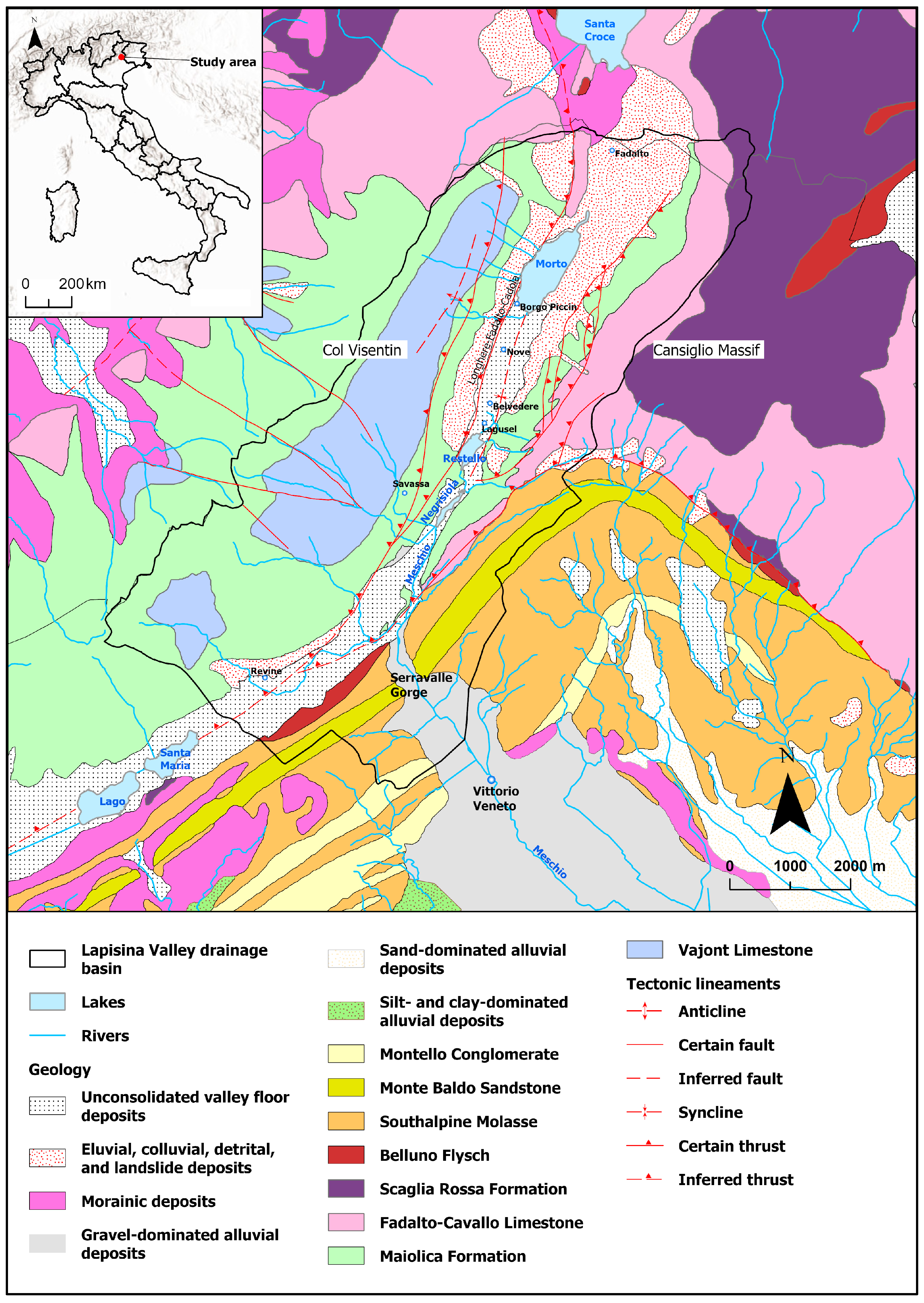
The evolution of the Lapisina Valley has been controlled by a structural depression situated between the Col Visentin ramp-anticline, which marks the eastern boundary of the Belluno Prealps, and the Cansiglio massif. The complex syncline forming the valley floor, displaced by a system of reverse and transcurrent faults associated with the Longhere–Fadalto–Cadola line, has predisposed the Lapisina Valley to develop as a transverse valley across the Prealpine range [33]. Both valley flanks are composed of a succession of Mesozoic calcareous rocks (Vajont Limestone, Maiolica Formation, and Fadalto Limestone), terminating with the Scaglia Rossa Formation (Lower Eocene–Upper Cretaceous). In the southeastern portion of the valley, this succession is locally and unconformably overlain by Tertiary rocks (Belluno Flysch, polygenic conglomerates, and Southalpine Molasse). The valley floor is covered by a blanket of unconsolidated deposits of eluvial, colluvial, detrital, morainic, glaciofluvial, and ancient-to-recent alluvial origin. In the northern sector, these deposits are not only thicker (approximately 65 m at Lagusel) but also coarser, consisting predominantly of gravel and sand. Moving toward the central and southern reaches, in addition to being thinner (20–30 m) [32], the sediments exhibit a finer grain size and are mainly composed of interbedded sands, silts, and clay (Figure 1).

From a hydrogeological perspective, the unconsolidated deposits host a phreatic aquifer, mainly recharged through interaction with the surface waters of the three lakes located on the valley floor and, to a lesser extent, by precipitation infiltration. The latter, estimated using the Thornthwaite & Mather [34] soil water balance and an infiltration coefficient of 30%, averaged 209.4 mm/year for the 1994–2022 period. The phreatic aquifer is bounded to the north by Morto Lake and to the east and west by rock outcrops. To the south, its extent is defined by the drainage divide separating the Lapisina Valley from the Soligo Valley near the village of Revine, as well as by the Serravalle Gorge, which connects the valley to the alluvial plain. Its base is defined by the contact with Mesozoic limestone, the variable depth of which was derived from geological cross-sections and available well logs. The prevailing groundwater flow direction in this aquifer is from NE to SW, from Morto Lake to the Serravalle Gorge, following the longitudinal development of the valley. Conversely, in its westernmost portion, between the Revine drainage divide and Serravalle, the flow is reversed (from SW to NE), consistent with the topographic gradient. The water table depth varies according to the topographic conditions, which are characterized by a terraced morphology developed on post-glacial landslide debris. In the lowest depressions and at slope breaks, groundwater emerges spontaneously, giving rise to spring zones (e.g., Lagusel and Belvedere). The Lapisina Valley phreatic aquifer is extensively exploited for drinking water supply through two well fields located at Borgo Piccin (adjacent to the southern shore of Morto Lake) and Lagusel, as well as by means of two drainage tunnels in the Belvedere locality.

2. Materials and Methods

2.1. Vulnerability Assessment

The intrinsic vulnerability was assessed by applying the SINTACS R5 method [24], a parametric point-rating and weighting system widely used both in Italy and internationally, with several applications across different hydrogeological contexts [35,36,37,38]. According to this method, seven parameters are considered to evaluate vulnerability: depth-to-water (S), recharge (I), impact of vadose zone (N), soil media (T), aquifer media (A), hydraulic conductivity (C), and slope (S).

The extent of the phreatic aquifer is discretized into a regular square-mesh grid overlaid on the base topographic map. The size of these Square Finite Elements (SFEs) typically depends on the available data and the morphology of the investigated area. For this case study, the SFEs have a side length of 10 m. Every evaluation is performed on individual SFEs to complete the required information matrix (scores, weights, and SINTACS index). Each of the seven parameters, divided into value ranges and/or specific categories, is assigned a score that increases according to its importance in the final overall assessment. Scores obtained for each parameter are multiplied by weighting strings that describe the local hydrogeological and/or impact scenario. The modular input structure of SINTACS was designed to accommodate various multiplier weighting strings, applied either alternatively or in parallel. These weighting lines serve as a powerful tool for tailoring the methodology to the local hydrogeological setting (impact scenario); they emphasize the relative importance of specific parameters while providing the analyst with a well-calibrated discretionary framework. The method accounts for five standard scenarios: normal impact, relevant impact, drainage, karst, and fractured. Based on the site’s hydrogeological characteristics and information extracted from geological, pedological, and land-use maps, two impact scenarios were assigned to the study area: relevant impact and drainage. The former accounts for territorial settings particularly prone to significant effects from potential diffuse pollution sources. These areas are characterized by an unsaturated zone mainly composed of unconsolidated deposits and are morphologically suitable for extensive human activity. Under these conditions, the unsaturated thickness plays a key role; thus, the weight string is designed to emphasize the parameters S, I, N, and T. The drainage scenario refers to areas where groundwater bodies are directly recharged by surface water bodies. In this case, great relevance is attributed to parameters A and C, highlighting the importance of fast transit times and the high propagation capacity of the aquifer. The northern portion of the domain, up to and including Negrisiola Lake, has been assigned the drainage scenario, given the presence of lakes that govern the exchange between surface water and groundwater. Meanwhile, the southern portion has been assigned the relevant impact scenario, given that nearly the entire valley floor is characterized by relatively uniform urban development, critical transport infrastructure (e.g., a motorway and a railway line), and agricultural areas where irrigation, fertilizers, and plant protection products are extensively applied. The southern area is also characterized by a shallow water table that increases vulnerability to potential pollution. The weighting strings applied to the SINTACS parameters for the two scenarios are reported in

Table 1. Weighting strings for relevant impact and drainage scenarios.

SINTACS Parameter	Relevant Impact	Drainage
S	5	4
I	5	4
N	4	4
T	5	2
A	3	5
C	2	5
S	2	2

.

To assess the intrinsic vulnerability of the aquifer using the SINTACS R5 method, each parameter was mapped in a GIS environment based on information collected from available reports and field data. The weights for the seven SINTACS parameters were calculated in parallel for each SFE, according to the respective hydrogeological/impact scenario. The final Intrinsic Vulnerability Index (IVI) was computed by aggregating the weighted parameter layers through an automated Python-based workflow (Python 3.14), using the Rasterio library to perform the raster calculations. This Python code is described in detail in the Supplementary Materials. The IVI is calculated as the sum of the products of each parameter’s score (P_j) and its respective weight (W_j), according to the following formula:

$$\mathrm{I}\mathrm{V}\mathrm{I}={\sum }_{\mathrm{j}=1}^7{(\mathrm{P}}_{\mathrm{j}}\times {\mathrm{W}}_{\mathrm{j}})$$

(1)

The obtained value is then normalized to a range between 0 and 100 to facilitate interpretation and cartographic representation according to vulnerability classes. These classes correspond to the normalized score intervals suggested by Italian legislation (Veneto Regional Government Decree 1621/2019), representing the following degrees of vulnerability: very low (Bb, 0 ÷ 25); low (B, 25 ÷ 35); moderate (M, 35 ÷ 50); high (A, 50 ÷ 70); very high (E, 70 ÷ 80); extremely high (Ee, 80 ÷ 100).

2.2. Hazard Assessment

In most cases, the assessment of the hazard component involves multiple actual or potential pollution sources, each characterized by distinct types and varying impact potentials. Furthermore, the duration of the exposure of the Subject at Risk (SAR) can span decades, often persisting long after the cessation of the activity that originally generated the pollutant. These factors complicate the construction of time series for pollution phenomena, hindering an accurate assessment of global risk [28]. Therefore, for long exposure times, the Territorial Hazard (H_T) value was set to coincide with the Hazard Index (HI) of the individual impact points. To determine HI values, the methodology proposed by Civita et al. [28] was applied, which utilizes the evaluation of Hazard Centers/Hazard Sources (HC/HS). Hazard centers or hazard sources are defined as point or diffuse anthropogenic activities that generate or could generate pollutants that may be transmitted to the local hydrogeological system. Hazard factors that contribute, individually or in combination, to classifying any anthropogenic activity as an HC/HS have been codified in previous work [39,40]. Specifically, these consist of seven hazard factors: special-purpose substances, hazardous substances, organic pollutant water discharges, inorganic pollutant water discharges, the handling and/or storage of potentially hazardous materials, water-intensive activities, and areal or linear pollution. Each hazard factor is assigned a score ranging from 0 to 3, based on the magnitude of the impact exerted on the SAR. The sum of these scores determines the overall hazard level of a specific anthropogenic structure or infrastructure, defined as the Hazard Index. Within the discretization grid, the hazard for each SFE is calculated by summing the HI values of all individual activities located within the cell, thereby generating the territorial hazard map.

For the Lapisina Valley, HC/HS data were obtained from databases provided by relevant public authorities, including the District Basin Authority, Genio Civile, the Veneto Region and the involved provinces and municipalities. This information was integrated with territorial data from other public sources (e.g., ARPAV) and satellite imagery (Google/Bing Maps). The identified HC/HS were then digitized within a GIS throughout the study area. Using the Raster Calculator tool in the GIS environment, each SFE was assigned a total hazard score. To classify the hazard levels, the calculated HI values for each SFE were analyzed using the Natural Breaks method [41], resulting in six hazard classes. It is important to note that a universal standard for hazard grades is not applicable to every territory, as the ranges were determined based on the frequency distribution of HI values within specific SFEs of the study area. Therefore, this subdivision remains site-specific.

2.3. Pollution Risk Assessment

To produce the Pollution Risk map, the risk assessment framework proposed by Civita et al. [28] was adopted, in which Risk (R) is defined by the following equation:

R = Vu_SAR × H_T × Va_SAR,

(2)

where Vu_SAR represents the intrinsic vulnerability of the Subject at Risk (SAR), H_T denotes the Territorial Hazard Factor, and Va_SAR signifies the value of the SAR. In this study, the SAR is represented by the phreatic aquifer of the Lapisina Valley. The methodology integrates these different factors within a GIS environment, maintaining a spatial discretization of the study area into SFEs with 10-m resolution. For the present study, the risk equation was applied to each individual SFE using the GIS Raster Calculator tool, multiplying vulnerability mapping (IVI values), hazard mapping (HI values) and the socio-economic value of the phreatic aquifer, yielding a risk score map. Regarding the Va_SAR factor, it was noticed that the aquifer is primarily exploited in its northern portion. Consequently, the study area was divided into two distinct sectors: a unit value (1.0) was assigned to the sector where groundwater is abstracted for drinking purposes, extending from Morto Lake to the northern limit of Negrisiola Lake, while a value of 0.5 was assigned to the remainder of the area. Following the same approach used for hazard classification, risk values were analyzed using the Natural Breaks method, resulting in four risk classes. As with the hazard assessment, this risk subdivision remains specific to the study area.

2.4. Stochastic Simulations Implementation

To derive the probabilistic factor of pollutant propagation, numerical simulations were performed to predict the movement of a generic contaminant within the study domain. Two widely adopted finite-difference numerical codes—MODFLOW-NWT [29] and MODPATH [30]—were used. These codes are part of the MODFLOW family developed by the United States Geological Survey (USGS) [42]. The former was used to reproduce groundwater flow and hydraulic head distributions under both steady-state and transient conditions. The simulations were calibrated automatically using the PEST code [43], based on field data collected during a 2023–2024 groundwater monitoring campaign. Subsequently, the advective transport component was simulated using MODPATH to reproduce the migration of pollutant particles in the absence of attenuation. This assumption was made in order to account for a generic contaminant in the framework and to provide a conservative worst-case representation of the system. Starting from the calibrated models, a stochastic approach was adopted to account for the uncertainty inherent in the modeling process. Indeed, the estimation of hydrogeological parameters, most notably hydraulic conductivity, is often subject to uncertainty due to the limitations of estimation methods and the discrete nature of available measurements (e.g., from wells or piezometers). While a deterministic approach yields a single solution representing the most likely estimate of the system, a stochastic approach generates an ensemble of simulations, each considered an equally probable realization of the modeled aquifer. This ensemble is then used to make predictions and estimate the probability or risk of specific scenarios. The GMS 10.5 software (AQUAVEO) served as the graphical interface for this procedure.

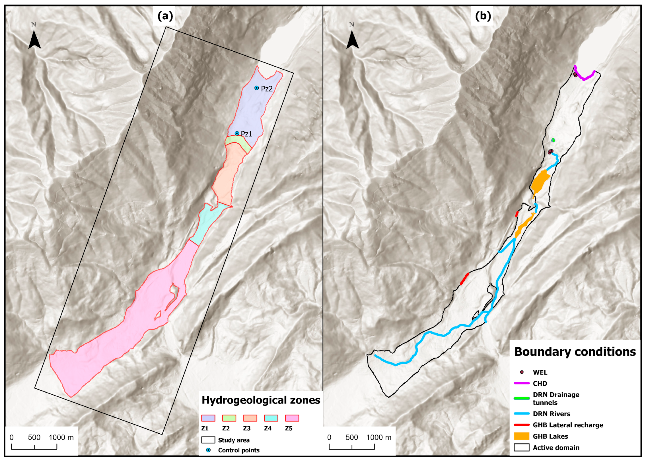
The modeling domain comprises the valley-floor deposits hosting the phreatic aquifer. To construct the discretization grid, a reference rectangle of 25.5 km² (3.0 km wide by 8.5 km long) was utilized. This rectangle was rotated 20° eastward from North, aligning it with the longitudinal axis of the valley. Within this area, a grid was generated with 10 m × 10 m cells, consisting of a total of 255,000 cells organized into 850 rows and 300 columns. Subsequently, cells located outside the polygon representing the outcrop area of the unconsolidated valley-floor deposits were deactivated. This resulted in 207,285 inactive cells and 47,715 active cells, with the active domain covering an area of 4.77 km². Regarding the vertical discretization, the phreatic aquifer is represented by a single layer of variable thickness. This layer is bounded by a bottom surface reconstructed from geological cross-sections and a top surface derived from the Veneto Region’s Digital Terrain Model (DTM) with a 5 m × 5 m resolution. The resulting cell thickness ranges from 20 to 230 m. The modeling domain was subdivided into five hydrogeological zones (Z1–Z5; Figure 2a). Each zone was characterized by distinct values of hydraulic conductivity (K) and effective porosity (n_e), the latter assumed to be equal to the specific yield (S_y) as a first approximation and used to calculate the velocity of advective transport particles. The calibrated values are reported in

Table 2. Calibrated values of K and S_y for each hydrogeological zone.

Hydrogeological Zones	K (m/d)	Sy (−)
Z1	135.55	0.30
Z2	6.18	0.20
Z3	18.08	0.30
Z4	17.28	0.20
Z5	17.28	0.20

, where the K value for Z1 was obtained as the average value of the hydraulic conductivity distribution within the zone, calculated using the pilot points method [44]. This method was applied only to Z1, where more information about K values is available, because it includes most of the observation points (3 piezometers out of a total of 5) and a well field. Hydrogeological stresses applied to the system were represented by the following boundary conditions (BCs, Figure 2b):

• The Time-variant Specified-Head (CHD) Package, a first-type BC, was used to simulate the interaction between groundwater and the surface water of Morto Lake;
• The Recharge (RCH) Package, a second-type BC, was used to simulate areal recharge resulting from precipitation infiltration;
• The Well (WEL) Package, a second-type BC, was used to simulate withdrawals from the Borgo Piccin and Lagusel wells fields;
• The Drain (DRN) Package, a third-type BC, was used to simulate discharge via the Belvedere and San Floriano drainage tunnels, as well as the groundwater/surface water interaction along the hydrographic network;
• The General-Head Boundary (GHB) Package, a third-type BC, was used to simulate the aquifer’s interaction with the surface water of Restello and Negrisiola lakes, as well as lateral recharge originating from groundwater circulation within the fractured rock masses of the Col Visentin slope.

For the estimation of recharge, the Thornthwaite & Mather soil water balance was applied to the study area for the monitoring period (2023–2024). This method provides an estimate of the average monthly surplus (P_e), which represents the amount of water on the soil surface available for infiltration and runoff. The P_e values were derived by analyzing precipitation and temperature data from the nearest meteorological stations. These values were then spatialized throughout the basin using a Multiquadratic Radial Basis Function (MRBF) [45]. Subsequently, the P_e values were multiplied by a potential infiltration coefficient (χ) of 30% to estimate monthly recharge. Spatialized monthly infiltration values were assigned to every stress period corresponding to a month of monitoring in the transient-state model, while the average recharge relative to the entire monitoring period was considered for the steady-state simulation.

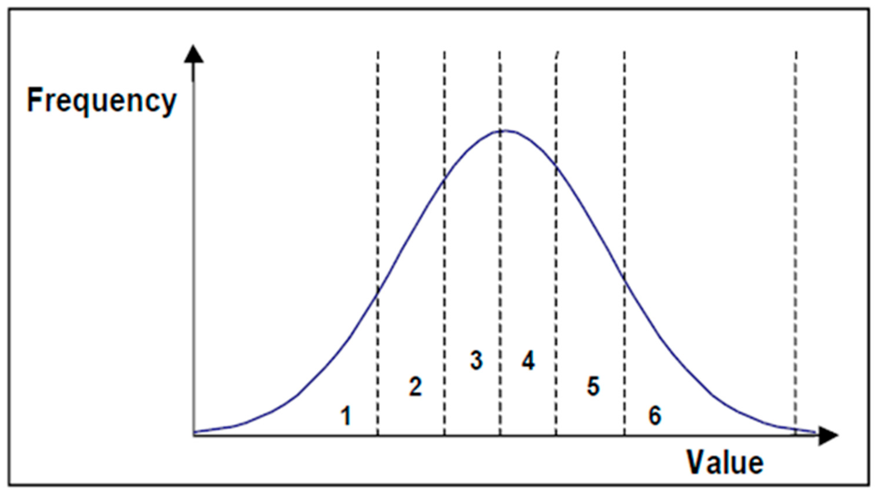
For parameter randomization, the Latin Hypercube Sampling (LHS) method was used [46,47]. This method requires the definition of a probability distribution and its associated statistical indicators (mean, standard deviation, minimum, and maximum values) for each analyzed model parameter. Additionally, it requires specifying the number of segments (n) into which the distribution must be divided. Consequently, the probability curve is partitioned into n intervals, each having an equal probability (i.e., the same area under the probability density function; Figure 3). Once the segments are defined, a value is randomly sampled from within each interval for every parameter. These values are then combined across parameters. The total number of simulations generated with this method corresponds to the product of the number of segments defined for each parameter. In this study, the LHS approach was applied to the five hydrogeological zones. Randomization was restricted to the steady-state flow simulation by varying hydraulic conductivity, excluding effective porosity due to its significantly lower variability relative to K. A normal probability distribution was assumed for the K parameters, partitioned into three segments, with the calibrated values serving as the mean. As a result, a total of 243 simulations were obtained (3⁵ = 243). Of these, 237 reached the convergence criterion, while six were discarded due to parameter combinations resulting in excessively high model error. The statistical indicators for the K randomization and n_e values associated with each hydrogeological zone are reported in

Table 3. Statistical indicators for the randomized parameter (K in m/d) across the five hydrogeological zones; std dev, standard deviation; min value, minimum value; max value, maximum value; n segments, number of segments; n_e, effective porosity values associated with each zone.

Statistical Parameters	Z1	Z2	Z3	Z4	Z5
K std dev	1.95	1.95	1.95	1.95	1.95
K average	135.55	6.18	18.08	17.28	17.28
K min	1.00 × 10−10	1.00 × 10−10	1.00 × 10−10	1.00 × 10−10	1.00 × 10−10
K max	10,000	10,000	10,000	10,000	10,000
n segments	3	3	3	3	3
ne (−)	0.30	0.20	0.30	0.15	0.15

.

2.5. Probabilistic Contaminant Propagation Factor

The innovative contribution of this study involves the introduction of a time-dependent probabilistic contaminant propagation factor, obtained through the implementation of stochastic simulations combined with the location of HC/HS. An advective transport particle was assigned to each cell of the domain intersected by one or more HC/HS. For each stochastic simulation generated using the LHS method, particle migration paths (pathlines) were calculated using the MODPATH code in forward mode, with travel times of 5, 10, 20, and 50 years. Pathlines for each simulation and travel time were then imported into a GIS environment. An automated cell-counting procedure was performed to identify cells intersected by the pathlines of a potential contaminant in each scenario. This process determined the probability of each cell being reached by potential contamination originating from HC/HS. This probability value is defined as the Probabilistic Contaminant Propagation Factor (P_CP(t)). This factor can assume values ranging from 0 to 1.

2.6. Contamination Risk Assessment

By combining the results of stochastic advective transport simulations with the pollution risk assessment, it was possible to generate four Contamination Risk maps for the study area. These were evaluated at 5, 10, 20, and 50 years from the moment a hypothetical contaminant, originating from one or more HC/HS, reaches the saturated zone. This approach attempts to reduce the uncertainty related to hydrogeological parameters by integrating the standard risk assessment with a probabilistic contaminant propagation factor. For the production of the maps, the values of P_CP (t) were multiplied by a normalized risk factor (R*) that can take on values of 0.25, 0.5, 0.75, and 1.0, assigned to the four pollution risk classes (low, moderate, high, and very high, respectively). Consequently, the Contamination Risk (R_C) is defined as follows:

R_C = P_CP (t) × R*

(3)

The R_C values range from 0 to 1. The four resulting maps serve as easily interpretable decision-making tools for both immediate responses following the detection of contamination events and long-term planning purposes.

3. Results

3.1. Intrinsic Vulnerability Map

The values for the S-SINTACS parameter (depth-to-water) were calculated for each SFE by subtracting the hydraulic head values (H) from the topographic elevation (Z). The Z values were derived from LIDAR data and integrated with the Veneto Region DTM. The H values were obtained by reconstructing the potentiometric surface of the phreatic aquifer through an MRBF, starting from the average hydraulic head values measured at monitoring points and hydrometric levels of lakes and main watercourses. The S values for each SFE, obtained from the difference between Z and H, were divided into ten intervals and assigned scores ranging from 1 to 10. The highest score relates to the shallowest depth-to-water values found in the south-central portion of the study area, at the lower elevations of the valley floor where the hydraulic head is roughly coincident with the hydrometric level of the surface hydrographic network, resulting in greater aquifer vulnerability. To determine the I-SINTACS parameter (recharge), the soil water balance for the 1994–2022 period was calculated within the Lapisina Valley drainage basin according to the Thornthwaite and Mather method. The point values of surplus calculated with this method were spatialized across the entire basin using an MRBF. The P_e values were subsequently multiplied by a potential infiltration coefficient (χ) assigned to each SFE based on the specific lithological cover, thus obtaining the values for parameter I. The scores for the different recharge intervals were assigned according to the authors’ guidelines, which specify that the maximum score (between 9 and 10) is assigned to the infiltration range of 250–300 mm/y; for higher values, the score tends to decrease to account for dilution and dispersion processes through the unsaturated zone. The highest scores are concentrated in the central and western parts of the study area. The N-SINTACS (impact of vadose zone) and A-SINTACS (aquifer media) parameters were evaluated based on the lithological and textural characteristics of the unsaturated zone and the deposits hosting the aquifer, respectively. The scores for these two parameters, assigned to each SFE, are higher in correspondence with coarser deposits (detrital and morainic), which are mainly found in the central and northern portions of the study area. The T-SINTACS parameter (soil media) was evaluated based on the pedological mapping available from ARPAV. In this case, the presence of clayey and silty textural classes is significant, as they possess high attenuation capacity, resulting in very low T-scores. Soil thickness is also of considerable importance because high T-scores are assigned to thin or absent soils, where the attenuation capacity is minimal or non-existent. The highest scores are found in the southern part of the study area and in correspondence with surface water bodies. To assign the scores for the C-SINTACS parameter (hydraulic conductivity), it was necessary to estimate the order of magnitude of K within the study area. The only known value was obtained through an aquifer test conducted at the Lagusel well field in October 2023, which yielded an order of magnitude of 10⁻³ m/s. This value was considered representative of the coarse deposits in the northern part of the domain. For the other hydrogeological units, the order of magnitude was evaluated based on the values provided by the SINTACS method for the indirect estimation, as a function of the hydrogeological complex hosting the aquifer. The maximum hydraulic conductivity values occur in the coarse detrital and morainic complexes, which correspond to high C-scores. Lower values were assigned to the predominantly fine complexes (silty-clayey-peaty and medium-fine moraines) present in the southwestern portion of the study area. Finally, to evaluate the S-SINTACS parameter (slope), a specific percentage slope value was assigned to each SFE. This value was derived from the DTM, and the relative score was obtained using the SINTACS function/graph. The score is very high in areas where the slope is gentle, corresponding to parts of the territory where surface runoff is limited, thereby promoting infiltration. Conversely, higher slopes favor runoff over infiltration, resulting in lower scores.

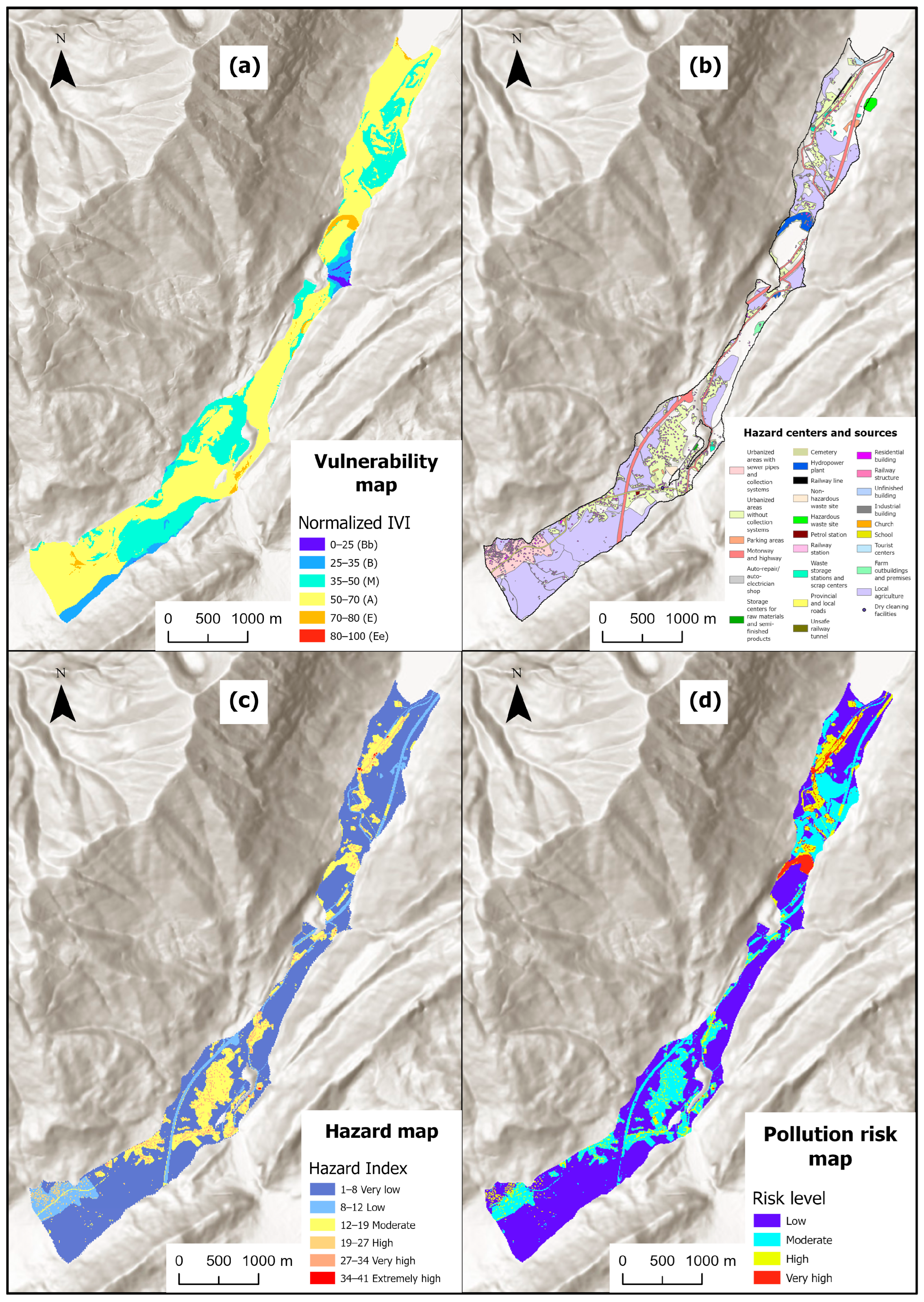
In the final vulnerability assessment, a normalized IVI value was derived for each SFE, enabling the construction of the vulnerability map shown in Figure 4a. No SFEs in the study area reached the Extremely High (Ee) threshold based on their IVI scores. The intrinsic vulnerability map clearly illustrates that areas with the highest vulnerability (E) are located near the Serravalle gorge, on the northern shore of Restello Lake, and on the southern shore of Morto Lake. This spatial pattern is primarily attributed to the influence of the S-SINTACS (depth-to-water) parameter in these areas, where the water table is found near the land surface. This provides a lower level of aquifer protection due to reduced attenuation processes and the short distance between the potential point of release (the ground surface) and the saturated zone. On the contrary, areas southeast of Restello Lake and south of Revine exhibit Very Low (Bb) to Low (B) vulnerability. This is due to the combination of low scores for the S-SINTACS parameter (indicating a significant depth to the water table) and low scores for the I-SINTACS parameter, resulting from the presence of lower-permeability lithotypes that hinder pollutants from reaching the saturated zone. Overall, most of the area falls into Moderate (M) and High (E) vulnerability classes, demonstrating that the water resource in the study area is highly sensitive to potential pollution events.

3.2. Hazard Map

• The hazard assessment procedure described above was applied to a list of anthropogenic activities and infrastructures categorized by the authors, along with the scores assigned to each hazard factor used to calculate the relative Hazard Index (HI). These activities represent potential hazard centers or sources to groundwater resources and are divided into three sectors (infrastructure, industrial, and agricultural).

The list was integrated for the present study with four additional categories of anthropogenic activities: dry cleaning facilities, hydropower plants, auto-repair/auto-electrician shops, and local agriculture. The categories of HC/HS identified within the study area are listed in

Table 4. List of HC/HS categories identified within the study area along with their relative HI values.

Sector	HC/HS	HI
Infrastructure	Urbanized areas with sewer pipes and collection systems	9
	Urbanized areas without collection systems	15
	Waste storage stations and scrap centers	8
	Underground storage tanks	15
	Petrol stations	11
	Motorways and highways	11
	Provincial and local roads	7
	Parking areas	11
	Railway lines	10
	Unsafe railway tunnels	9
	Railway stations	9
	Tourist centers	6
	Cemeteries	4
Industrial	Storage centers for raw materials and semi-finished products	12
	Non-hazardous waste sites	7
	Hazardous waste sites	18
Agricultural	Farm outbuildings and premises	4
Additional categories	Dry cleaning facilities	9
	Hydropower plants	3
	Auto-repair/auto-electrician shops	13
	Local agriculture	7

, along with the relative HI value calculated according to the methodology.

All the collected and identified HC/HS were digitized within a GIS environment throughout the study area, resulting in a total of 1656 polygons and 1 point feature. Regarding the potential hazard source related to heating oil tanks, under the underground storage tanks category, it was not possible to retrieve site-specific information. Due to the lack of a natural gas distribution system and considering that heating oil remains the most widely used fuel in mountain towns, all residential, civil, and industrial buildings were extracted from the Regional Technical Map (CTR) in vector format. As a precautionary measure, HI corresponding to the underground storage tanks category was assigned to each of these buildings. All the classified HC/HS used for the hazard assessment are reported in the map in Figure 4b. The HC/HS categories with the highest HI scores in the study area are as follows: hazardous waste sites (18), with an area located in the northeastern part of the domain; urbanized areas without collection systems (15), represented by all the inhabited centers in the municipality of Vittorio Veneto; underground storage tanks (15), assigned to every residential, civil, and industrial building in the study area; auto-repair/auto-electrician shops (13) and storage centers for raw materials and semi-finished products (12), represented by two areas located in Savassa Bassa along the SS51 highway and the railway line, respectively.

Finally, the hazard value for each individual SFE was calculated as the sum of the HI values assigned to the individual HC/HS present within it, which produced the hazard map presented in Figure 4c, where the total HI values, subdivided into six classes using the Natural Breaks method, range from a minimum of 3 to a maximum of 41. The maximum hazard class (extremely high) is concentrated in small portions of the territory characterized by the presence of industrial buildings with attached waste storage centers, as well as the disused railway station complex of Nove. The assignment of the HI value related to the potential presence of heating oil tanks to all residential and industrial buildings results in a high hazard level in correspondence with these structures. Generally, in the main inhabited centers of the valley, the hazard is moderate due to the absence of a unified sewage collection system. Other hazard sources that cannot be overlooked include hydropower plants, the motorway, and the railway.

3.3. Pollution Risk Map

The groundwater Pollution Risk map for the Lapisina Valley, generated using the risk Formula (2), is shown in Figure 4d. Areas exhibiting the highest risk, from High to Very High, are primarily located in the northern portion of the study area. In this sector, the use of groundwater for drinking purposes inherently assigns it a higher social/resource value than in the southern portion. Furthermore, the convergence of intrinsically vulnerable areas and concentrated HC/HS explains this high-risk pattern, which requires specific management attention. In particular, the highest-risk zones are the area of the Restello Lake hydropower plant, on its northern shore, and the village of Nove along the SS51 highway.

3.4. Stochastic Simulations

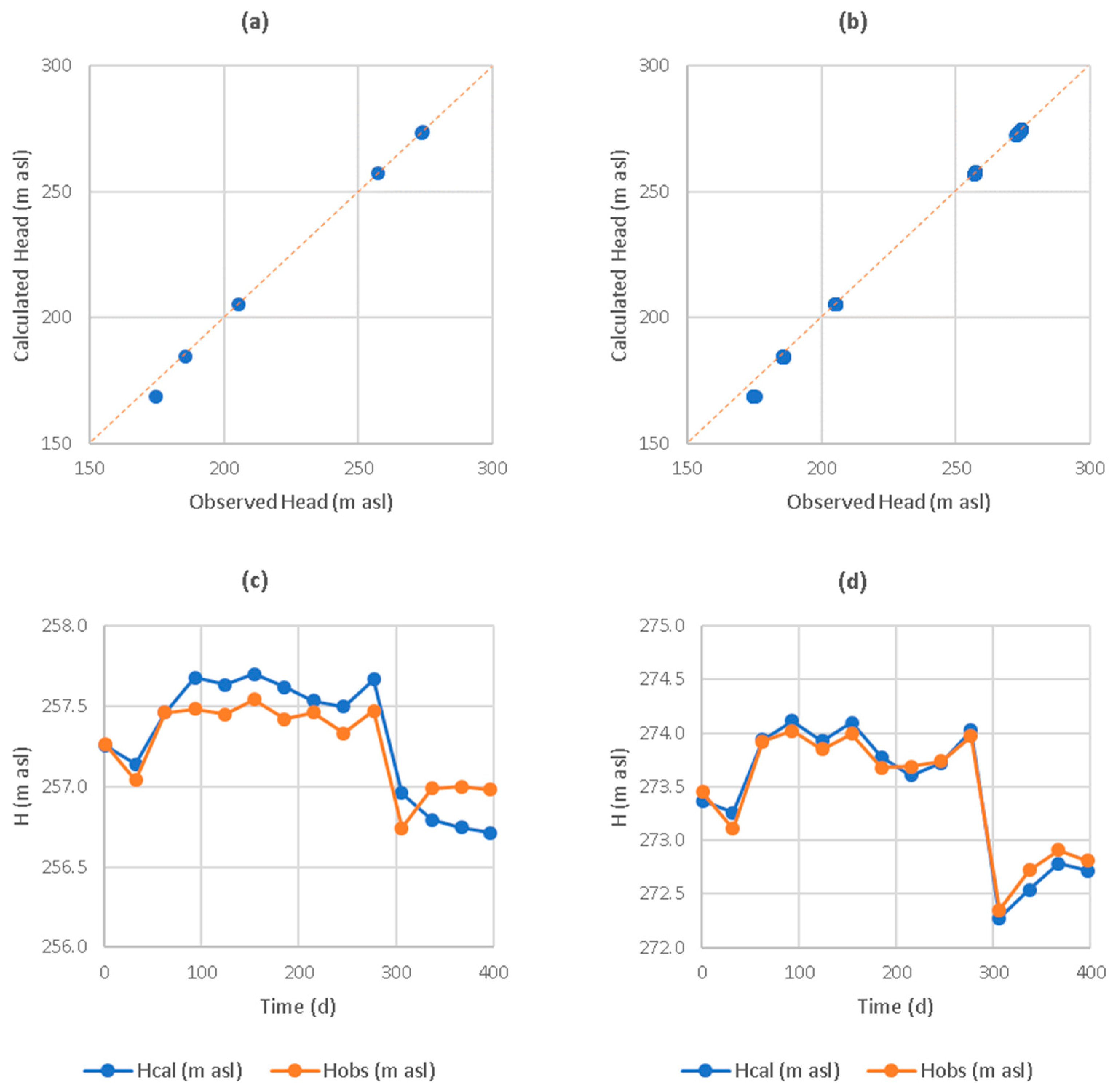
The steady-state calibration simulation satisfactorily reproduced the average hydraulic head values measured at the monitoring points during the hydrogeological survey conducted from May 2023 to May 2024. This is shown in the scatter plot in Figure 5a, which compares measured head values with those calculated by the model. The graph shows a good model fit, as indicated by a Coefficient of Determination (R²) of nearly 1 (0.996) and a Normalized Root Mean Square Error (NRMSE) of 2.58%. The transient-state calibration simulation also yielded good results, in this case reproducing the monthly average H values for the thirteen months of monitoring. The comparison between observed and calculated values can be seen in the scatter plot in Figure 5b, which shows high goodness-of-fit with an R² of nearly 1 (0.998) and an NRMSE of 1.76%, while Figure 5c,d show the trend of the monthly average measured and calculated values during the monitoring period at two control points: the piezometers designated Pz1 and Pz2, located in the Pian dei Nove area between Restello Lake and Morto Lake (see Figure 2a). The calibrated parameters (K and S_y) served as the basis for developing flow and advective transport simulations using the stochastic approach, as described in Section 2.

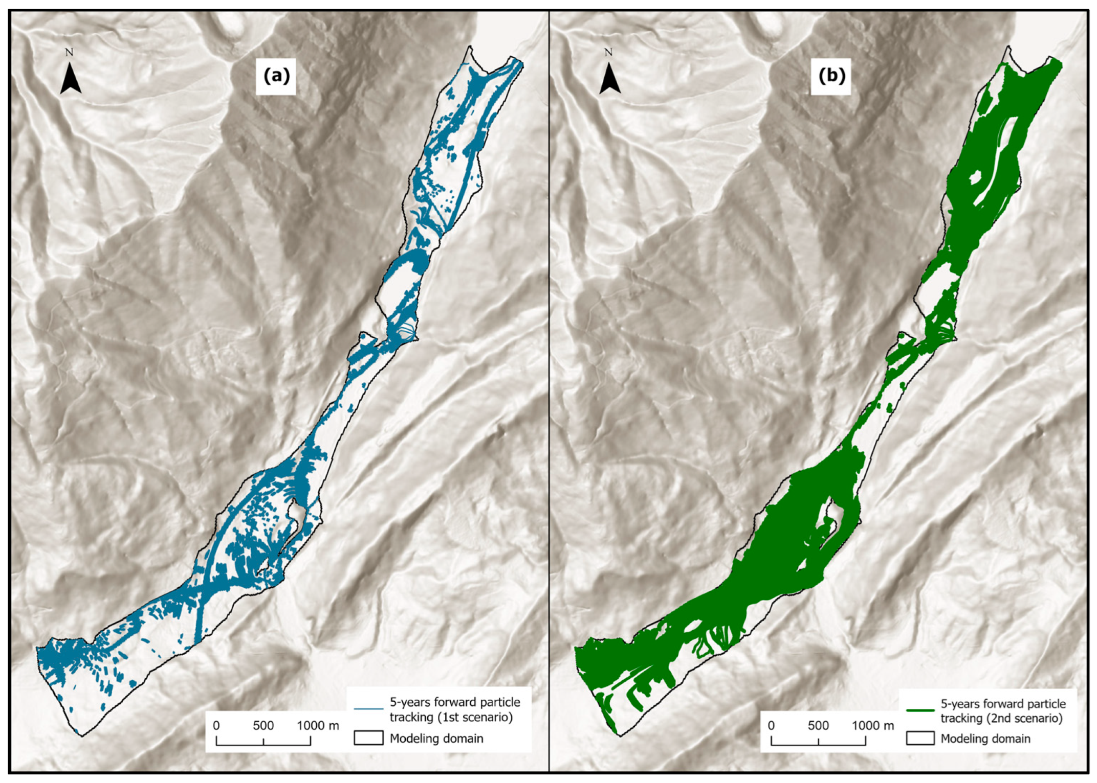
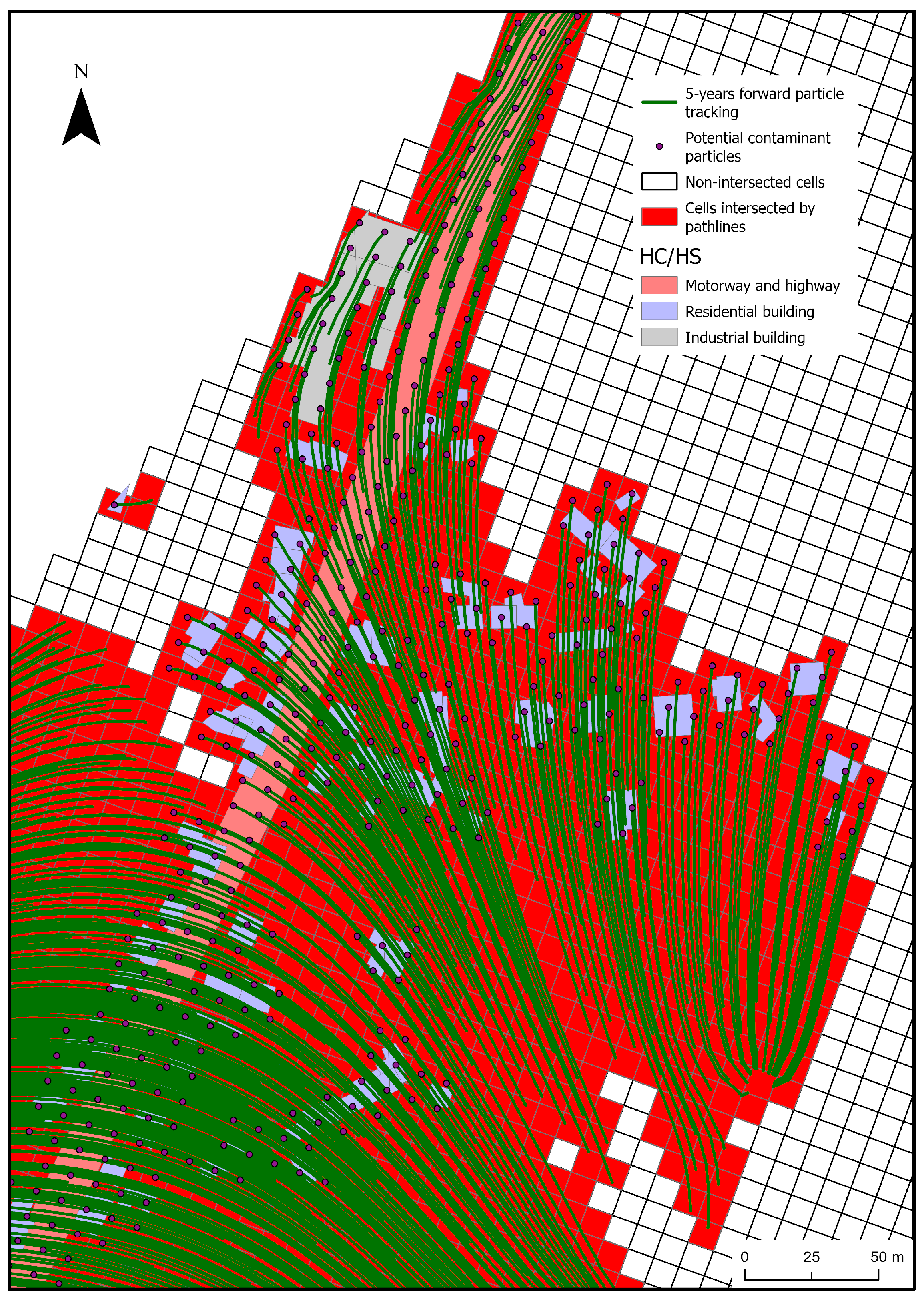
The shapefiles related to the HC/HS were imported into the GMS 10.5 software, except for the hazard sources falling under the following categories: urbanized areas with sewer pipes and collection systems, urbanized areas without collection systems, local agriculture, tourist centers, and farm outbuildings and premises. These categories were excluded because they represent very extensive diffuse non-point sources and were therefore considered poorly representative when modeled as point sources of potential contamination. Subsequently, an advective transport particle was assigned to each cell of the domain intersected by one or more HC/HS, with an initial position of the particle on the water table surface. For each of the 237 converged stochastic simulations, pathlines were generated in forward mode with travel times of 5, 10, 20, and 50 years. By considering many potential hydrogeological scenarios, the particle-tracking outcomes can similarly follow different trends and cover different portions of the study area. Two examples are illustrated in Figure 6, showing pathlines with a travel time of 5 years. To determine the probability of a specific point within the domain being reached by one or more contaminant particles, the set of tracking scenarios was treated as an ensemble of all possible realizations of the potential contamination. Subsequently, an automated counting methodology was applied within a GIS environment. For each scenario, the cells of the discretization grid intersected by one or more pathlines were selected, as illustrated in Figure 7. A unit value (1) was assigned to these cells to indicate the occurrence of potential contamination. The sum of the occurrences across all scenarios was divided by the total number of realizations (237). This ratio determines the probability (P_CP) of a cell or SFE being reached by potential contamination. The counting procedure was applied to each of the four travel times (5, 10, 20, and 50 years), generating four raster files containing the probability values of contaminant propagation.

3.5. Contamination Risk Maps

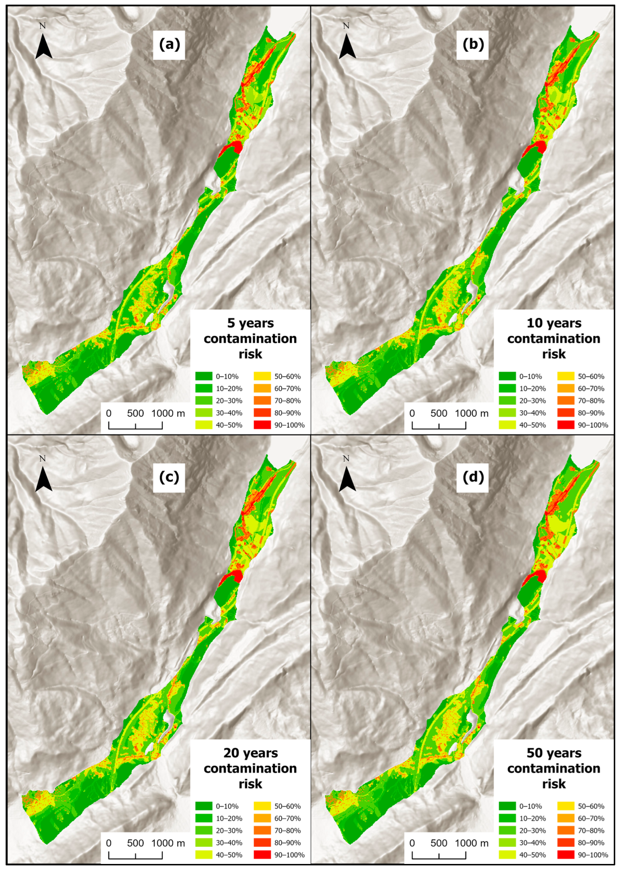
To generate the groundwater Contamination Risk maps, the four risk classes from the Pollution Risk map, originally calculated using the Natural Breaks method, were replaced with probabilistic weighting values of 0.25, 0.5, 0.75, and 1.0, respectively. In a GIS environment, the reclassified pollution risk raster was multiplied by each of the raster containing the contaminant propagation probability data for 5, 10, 20, and 50 years. This process yielded four new rasters where the cell values correspond to the Contamination Risk (R_C) values. Cell values of the four final rasters were classified into 10 risk classes using equal intervals of 0.1. The resulting Contamination Risk maps, illustrated in Figure 8, depict temporal scenarios at 5, 10, 20, and 50 years following the potential arrival of a hypothetical contaminant in the saturated zone. These outputs provide essential information for land management and groundwater resource protection. Compared to the static pollution risk map, these dynamic maps offer insights into contamination propagation, obtained by stochastically simulating the advective transport of a hypothetical contaminant. This approach is inherently conservative, as it neglects attenuation phenomena such as dispersion, adsorption, and degradation. Furthermore, the integration of the time variable enables the evaluation of multiple future scenarios. As observed, there are no substantial differences in the areas exhibiting a very high risk degree (70–100%), which are primarily located in the northern portion of the study area where drinking water extraction points are concentrated. Specifically, the highest-risk zones are the industrial area of the Restello Lake hydroelectric plant and the residential center of Nove along the SS51 highway, including the disused railway station complex. This highlights that areas characterized by high intrinsic vulnerability and concentrated hazard sources require prioritized attention, irrespective of the considered propagation timeframe. The differences between the four scenarios mainly involve a progressive increase in areas with moderate-to-high propagation risk (30–70%). This distribution is more localized (point-based) than areal, due to the presence of private homes with heating oil tanks and, in some cases, the lack of a collective sewer system, both of which are identified as potential hazard sources. Finally, both the A27 motorway and the railway line are identified as high-risk (50–70%) features in all four scenarios.

4. Discussion

In the literature, several scientific studies utilize numerical modeling to define or validate groundwater vulnerability and risk. In most cases, however, simulations are conducted using a deterministic approach based on single scenarios, while stochastic procedures aimed at deriving a probabilistic contaminant propagation factor, as presented in this article, are rarely adopted.

One of the earliest examples of integrating modeling and risk assessment is represented by the work of Nobre et al. [48]. In this study, the authors calculate risk as the product of three components: intrinsic vulnerability, derived using the DRASTIC method; potential contamination sources, identified through a fuzzy hierarchical model; and a well index, calculated based on the delineation of capture areas through deterministic steady-state simulations with MODFLOW-96 and MODPATH. Similarly, in Baalousha [49], groundwater contamination risk is mapped by combining four different thematic layers: intrinsic vulnerability calculated using the DRASTIC method, land use, drinking water well capture areas delineated through a deterministic steady-state simulation with MODFLOW/PMPATH, and finally, the impact distribution of nitrates, chlorides, and fluorides. Both examples share the common goal of identifying protection areas for drinking water wells, which typically involve performing a particle-tracking analysis in backward mode. In contrast, the current study utilizes forward particle tracking, moving from the potential contamination source downgradient along the groundwater flow direction. This approach is therefore not limited to localized assessments of specific sectors but encompasses the entire study area, identifying the probability of contaminant propagation. An example of the use of forward particle-tracking analysis, coupled with a vulnerability assessment of a wetland to a hypothetical subsurface contaminant spill, is presented by Gárfias et al. [50]. In this case, however, the authors limit their approach to the implementation of several deterministic steady-state simulations using MODFLOW-2005 and MODPATH codes, as well as the evaluation of the effectiveness of hypothetical protection measures.

More recently, Vu et al. [51] used deterministic steady-state simulations, implemented with MODFLOW-2000, to refine an intrinsic vulnerability assessment conducted with the modified-AHP-DRASTIC method [52], thus integrating the potential effects of climate change on groundwater circulation. Similarly, in Zhao et al. [53], the intrinsic vulnerability calculated using the modified-AHP-DRASTIC method is coupled with the results of a deterministic transient-state flow and transport simulation, conducted with MODFLOW and MT3DMS codes, to derive a groundwater contamination risk map. In this study, two target contaminants were used: manganese and chlorides. A similar approach is presented in Eslamian et al. [23], where the intrinsic vulnerability calculated with the DRASTIC method is optimized based on the results of deterministic simulations conducted with MODFLOW for flow and MT3DMS for nitrate transport. Finally, in one of the most recent studies [54], a deterministic coupled surface–groundwater flow simulation, conducted with the SWAT and MODFLOW-NWT codes, is used to define three of the seven parameters of the DRASTIC method (depth-to-water, recharge, and hydraulic conductivity).

Regarding simulations with a stochastic approach, one of the earliest examples is the work of Jafari et al. [55]. In this study, groundwater contamination risk is identified by combining intrinsic vulnerability (DRASTIC method) with a probabilistic contamination factor; the latter is calculated through flow (MODFLOW) and nitrate transport (MT3DMS) simulations governed by the Monte Carlo technique and based on an initial deterministic calibration. This represents one of the first contributions where the integration of probability allows for more realistic risk maps compared to those derived from simple intrinsic vulnerability assessments. This approach was further refined by Soriano et al. [56], who utilized stochastic steady-state simulations conducted with MODFLOW 6 and MODPATH-7. Using the iterative ensemble smoother (PESTPP-IES) included in the PEST++ version 5 suite, the authors evaluated the ability of two different parameterization scenarios, one based on zones and the other on pilot points, to match simulated values with calibration targets, following a Monte Carlo-type approach. The best-calibrated scenarios were subsequently used for a forward particle-tracking analysis starting from the locations of unconventional hydrocarbon extraction sites, following a methodology similar to the one presented in this article. The final result is the calculation of a probabilistic vulnerability index, defined by the ratio between the number of realizations in which a particle intersects a given location and the total number of realizations. This assessment, however, remains limited to the presence of unconventional hydrocarbon extraction sites.

The methodology proposed in this article for calculating P_CP(t) is highly flexible, as it can also be implemented using other codes such as MODFLOW 6 [57,58] or FEFLOW [59] for flow, and mod-PATH3DU [60] or Ichnos [61] for advective particle tracking. The deterministic phase of the simulations (calibration) aims to determine the characteristic values of the probability distributions for the parameters to be randomized (K), or to identify realistic values for those not subject to the stochastic procedure (n_e). In the present case, randomization concerned only the hydraulic conductivity, as it is the parameter that potentially exhibits the highest range of variability; however, the same procedure is extendable to effective porosity and recharge, enabling a further reduction in uncertainty in pollutant propagation. The probability distribution identified in this study is normal, but the approach allows for the use of other probability density functions, such as log-normal. Sampling methods can also be varied, using, for example, random sampling [62] as an alternative to Latin Hypercube, and the number of sectors can be customized. Similarly, the count of cells intersected by the pathlines, performed here via ArcGIS Pro 3.6 (ESRI), can be implemented in any GIS environment (e.g., QGIS, SAGA). It should be noted that particle -tracking simulations were implemented excluding some extensive diffuse non-point hazard sources due to representational constraints. For the Lapisina Valley case study, point sources were considered sufficiently representative; however, applying the methodology in areas characterized by a predominance of diffuse sources might also necessitate the modeling of the latter. The probabilistic propagation factor presented here was associated with the risk assessment methodology proposed by Civita et al. [28], although it can be easily integrated into other calculation procedures, such as those based on intrinsic vulnerability calculated with the DRASTIC method. Furthermore, the introduction of travel time into the particle-tracking analysis transforms the tool from a static to a dynamic one, overcoming one of the primary inherent limitations of classical groundwater contamination risk assessments [31]. Although accounting exclusively for advection provides a conservative worst-case framework, neglecting attenuation processes, such as dispersion, adsorption, and degradation, may lead to an overestimation of the spatial extent and persistence of contamination, particularly for reactive compounds. Future developments of this research should incorporate reactive transport into stochastic modeling, using transport codes such as MT3DMS [63] or RT3D [64] to address specific contaminants or categories of contaminants. Such a transition from non-reactive to reactive transport necessitates a fundamental shift in assessment methodologies: moving from intrinsic to specific vulnerability and narrowing the scope of hazard sources to those specifically associated with the release of the target substance or chemically analogous groups. The proposed methodology is applicable in all contexts characterized by porous aquifers. For different hydrogeological settings, such as those dominated by karst or fractured media, the transferability of the method should be verified by taking their specific characteristics into account. Regarding karst systems, they require specific tools for vulnerability and risk assessment and for modeling implementation; therefore, this method is not directly applicable. In contrast, where fractured media can be treated using the equivalent porous medium approach (EPM), this allows the application of the method proposed in this article to be feasible.

5. Conclusions

Groundwater resources represent a vital strategic asset for society and are essential for human consumption and productive uses; therefore, they must be safeguarded to ensure sustainable exploitation. The present study introduced an integrated and dynamic approach to groundwater risk assessment, moving beyond the static nature of traditional overlay-index methods. By coupling the established SINTACS framework with stochastic numerical modeling, the research successfully incorporated an innovative time-dependent predictive tool into the decision-making process. The proposed methodology enabled the introduction of a Probabilistic Contaminant Propagation Factor (P_CP(t)) into the contamination risk assessment. This factor represents the primary innovative contribution of the study, providing dynamism to traditional risk assessment by integrating stochastic probability and the temporal dimension. The final output of this framework was the generation of Contamination Risk maps for 5-, 10-, 20-, and 50-year travel times. These maps provide essential insights for emergency management and short-to-long-term territorial planning, identifying the most probable high-risk flow paths. While high-risk zones (70–100%) remain relatively stable in the northern part of the Lapisina Valley study area (where the main drinking water abstraction points are located), specifically near industrial areas, hydropower plants, and key infrastructure like the A27 motorway and the railway, the areas of moderate-to-high risk (30–70%) expand significantly over time. This evolution underscores the significance of a tool capable of evaluating future scenarios across various timesteps while incorporating the inherent uncertainty of hydrogeological parameters.

From the perspective of sustainable land and water resource management, the proposed tool is applicable at various levels. For planning purposes, it allows for identifying low-risk areas for the construction of new abstraction wells or, conversely, preventing an increased risk in already vulnerable areas by restricting potentially hazardous activities. Furthermore, it assists in emergency management in the event of active contamination. Indeed, the dynamic mapping enables the timely identification of sectors subject to contaminant propagation, facilitating both the design of an optimized monitoring network and the strategic placement of emergency mitigation measures. It should be emphasized that the proposed workflow is highly flexible, as the various steps, from vulnerability and hazard assessment to the implementation of numerical simulations, can be adapted to specific management needs and diverse hydrogeological settings. In particular, the number of stochastic realizations can be significantly increased by modifying the input parameters of the randomization method. This would allow for a further reduction in the uncertainty associated with hydrogeological parameters, enhancing the statistical robustness of the probability distribution. In conclusion, the hybrid methodology presented here provides a scientifically grounded and easily interpretable decision-making tool. While the current model is intentionally conservative due to focusing on advective transport, it offers a robust worst-case scenario framework.

References

1. Shiklomanov, I.A.; Rodda, J.C. World Water Resources at the Beginning of the Twenty-First Century; Cambridge University Press: Cambridge, UK, 2003. [Google Scholar]
2. UNESCO. The United Nations World Water Development Report 2022: Groundwater: Making the Invisible Visible; UNESCO Publishing: Paris, France, 2022. [Google Scholar]
3. EEA. Europe’s Groundwater—A Key Resource Under Pressure; European Environment Agency: Copenhagen, Denmark, 2022. [Google Scholar]
4. ISTAT. Le Statistiche Dell’istat Sull’acqua. Anni 2020–2024; Istituto Nazionale di Statistica: Roma, Italy, 2024. [Google Scholar]
5. Pistocchi, A. (Ed.) Ecological and Human Health Risk Assessment: Focusing on Complex Chemical Risk Assessment and the Identification of Highest Risk Conditions; Report No. EUR 22625 EN; Institute for Environment and Sustainability, Joint Research Centre, European Commission: Ispra, Italy, 2006; 132p. [Google Scholar]
6. Lahr, J.; Kooistra, L. Environmental risk mapping of pollutants: State of the art and communication aspects. Sci. Total Environ. 2010, 408, 3899–3907. [Google Scholar] [CrossRef] [Scilit]
7. Vrba, J.; Zaporozec, A. Guidebook on Mapping Groundwater Vulnerability; H. Heise: Hannover, Germany, 1994. [Google Scholar]
8. National Research Council. Groundwater Vulnerability Assessment: Contamination Potential Under Conditions of Uncertainties; National Academy Press: Washington, DC, USA, 1993; 185p. [Google Scholar]
9. Taghavi, N.; Niven, R.K.; Paull, D.J.; Kramer, M. Groundwater vulnerability assessment: A review including new statistical and hybrid methods. Sci. Total Environ. 2022, 822, 153486. [Google Scholar] [CrossRef] [Scilit]
10. Gogu, R.; Dassargues, A. Current trends and future challenges in groundwater vulnerability assessment using overlay and index methods. Environ. Geol. 2000, 39, 549–559. [Google Scholar] [CrossRef] [Scilit]
11. Pavlis, M.; Cummins, E.; McDonnell, K. Groundwater vulnerability assessment of plant protection products: A review. Hum. Ecol. Risk. Assess. 2010, 16, 621–650. [Google Scholar] [CrossRef] [Scilit]
12. Shirazi, S.M.; Imran, H.M.; Akib, S. GIS-based DRASTIC method for groundwater vulnerability assessment: A review. J. Risk Res. 2012, 15, 991–1011. [Google Scholar] [CrossRef] [Scilit]
13. Sorichetta, A.; Ballabio, C.; Masetti, M.; Robinson, G.R.; Sterlacchini, S. A comparison of data-driven groundwater vulnerability assessment methods. Groundwater 2013, 51, 866–879. [Google Scholar] [CrossRef] [Scilit]
14. Ivan, V.; Madl-Szonyi, J. State of the art of karst vulnerability assessment: Overview, evaluation and outlook. Environ. Earth Sci. 2017, 76, 25. [Google Scholar] [CrossRef] [Scilit]
15. Goyal, D.; Haritash, A.K.; Singh, S.K. A comprehensive review of groundwater vulnerability assessment using index-based, modelling, and coupling methods. J. Environ. Manag. 2021, 296, 113161. [Google Scholar] [CrossRef] [Scilit]
16. Aller, L.; Bennet, T.; Lehr, J.H.; Petty, R.J. DRASTIC: A Standardized System for Evaluating Groundwater Pollution Potential Using Hydrogeologic Settings; U.S. EPA Report 600/2-85/018; U.S. Environmental Protection Agency: Washington, DC, USA, 1987.
17. Al-Adamat, R.A.; Foster, I.D.; Baban, S.M. Groundwater vulnerability and risk mapping for the Basaltic aquifer of the Azraq basin of Jordan using GIS, remote sensing and DRASTIC. Appl. Geogr. 2003, 23, 303–324. [Google Scholar] [CrossRef] [Scilit]
18. Panagopoulos, G.P.; Antonakos, A.K.; Lambrakis, N.J. Optimization of the DRASTIC method for groundwater vulnerability assessment via the use of simple statistical methods and GIS. Hydrogeol. J. 2006, 14, 894–911. [Google Scholar] [CrossRef] [Scilit]
19. Rahman, A. A GIS based DRASTIC model for assessing groundwater vulnerability in shallow aquifer in Aligarh, India. Appl. Geogr. 2008, 28, 32–53. [Google Scholar] [CrossRef] [Scilit]
20. Neshat, A.; Pradhan, B.; Dadras, M. Groundwater vulnerability assessment using an improved DRASTIC method in GIS. Resour. Conserv. Recycl. 2014, 86, 74–86. [Google Scholar] [CrossRef] [Scilit]
21. Khosravi, K.; Sartaj, M.; Tsai, F.T.C.; Singh, V.P.; Kazakis, N.; Melesse, A.M.; Prakash, I.; Bui, D.T.; Pham, B.T. A comparison study of DRASTIC methods with various objective methods for groundwater vulnerability assessment. Sci. Total Environ. 2018, 642, 1032–1049. [Google Scholar] [CrossRef] [Scilit] [PubMed]
22. Patel, P.; Mehta, D.; Sharma, N. A review on the application of the DRASTIC method in the assessment of groundwater vulnerability. Water Supply 2022, 22, 5190–5205. [Google Scholar] [CrossRef] [Scilit]
23. Eslamian, S.; Harooni, Y.; Sabzevari, Y. Simulation of nitrate pollution and vulnerability of groundwater resources using MODFLOW and DRASTIC models. Sci. Rep. 2023, 13, 8211. [Google Scholar] [CrossRef] [Scilit]
24. Civita, M.V.; De Maio, M. Valutazione e Cartografia Automatica Della Vulnerabilità Degli Acquiferi All’ Inquinamento con il Sistema Parametrico: SINTACS R5, a New Parametric System for the Assessment and Automaticmap Ping of Groundwater Vulnerability to Contamination; Pitagora Editrice: Bologna, Italy, 2000; p. 240. [Google Scholar]
25. Civita, M.V.; De Maio, M. Assessing and mapping groundwater vulnerability to contamination: The Italian combined approach. Geofis. Int. 2004, 43, 513–532. [Google Scholar] [CrossRef] [Scilit]
26. Civita, M.V. The Combined Approach When Assessing and Mapping Groundwater Vulnerability to Contamination. J. Water Resour. Prot. 2010, 2, 14–28. [Google Scholar] [CrossRef]
27. Nguyet, V.T.M.; Goldscheider, N. A simplified methodology for mapping groundwater vulnerability and contamination risk, and its first application in a tropical karst area, Vietnam. Hydrogeol. J. 2006, 14, 1666–1675. [Google Scholar] [CrossRef] [Scilit]
28. Civita, M.V.; Sappa, G.; Zavatti, A. Una procedura di valutazione delle fonti di pericolo per le acque sotterranee. IGEA-Ing. Geol. Degli Acquiferi 2005, 20, 59–68. [Google Scholar]
29. Niswonger, R.G.; Panday, S.; Ibaraki, M. MODFLOW-NWT, a Newton formulation for MODFLOW-2005. In U.S. Geological Survey Techniques and Methods; U.S. Geological Survey: Reston, VA, USA, 2011; Volume 6-A37, 44p. [Google Scholar]
30. Pollock, D.W. User Guide for MODPATH Version 7—A Particle-Tracking Model for MODFLOW; U.S. Geological Survey Open-File Report; U.S. Geological Survey: Reston, VA, USA, 2016; Volume 1086, 35p. [CrossRef] [Scilit]
31. Ducci, D.; De Masi, G.; Priscoli, G. Contamination risk of the Alburni karst system (southern Italy). Eng. Geol. 2008, 99, 109–120. [Google Scholar] [CrossRef] [Scilit]
32. Avigliano, R.; Poli, M.E.; Zanferrari, A. Buried architecture of the Quaternary Vittorio Veneto basin (NE Italy). Boll. Geofis. Teor. Appl. 2008, 49, 357–368. [Google Scholar]
33. Pellegrini, G.B.; Surian, N. Geomorphological study of the Fadalto landslide, Venetian Prealps, Italy. Geomorphology 1996, 15, 337–350. [Google Scholar] [CrossRef] [Scilit]
34. Thornthwaite, C.W.; Mather, J.R. Instructions and Tables for Computing Potential Evapotranspiration and the Water Balance, 10; Laboratory of Climatology, C.W. Thornthwaite Associates: Elmer, NJ, USA, 1957. [Google Scholar]
35. Al Kuisi, M.; El-Naqa, A.; Hammouri, N. Vulnerability mapping of shallow groundwater aquifer using SINTACS model in the Jordan Valley area, Jordan. Environ. Geol. 2006, 50, 651–667. [Google Scholar] [CrossRef] [Scilit]
36. Sahu, I.; Prasad, A.D.; Ahmad, I. Comparison of GIS-Based Intrinsic Groundwater Vulnerability Assessment Methods: DRASTIC and SINTACS. Nat. Environ. Pollut. Technol. 2022, 21, 2249–2258. [Google Scholar] [CrossRef] [Scilit]
37. Sadri, S.; Radmanesh, F.; Ahmadpari, H.; Ladez, B. Pollution potential assessment of Jarmeh plain groundwater with use of SINTACS and DRASTIC models in GIS media. In Proceeding of the 4th International Congress of Developing Agriculture, Natural Resources, Environment and Tourism of Iran; Tabriz Islamic Art University: Tabriz, Iran, 2019. [Google Scholar]
38. Ourarhi, S.; Barkaoui, A.E.; Zarhloule, Y. Groundwater vulnerability assessment in the Triffa Plain based on GIS combined with DRASTIC, SINTACS, and GOD models. Arch. Environ. Prot. 2023, 49, 50–58. [Google Scholar] [CrossRef] [Scilit]
39. Tacconi, E.; Zavatti, A. Indici Ponderati Relativi di Pressione delle Attività Antropiche; ARPA Emilia-Romagna: Bologna, Italy, 1999; documento inedito. [Google Scholar]
40. Civita, M.V.; Sappa, G. Applicazione di una metodologia innovativa per la valutazione del pericolo di contaminazione delle risorse idriche sotterranee. In Proceedings of the National Conference on Groundwater Protection and Management, Reggia di Colorno, Italy, 15–17 September 2005. [Google Scholar]
41. Jenks, G.F. The Data Model Concept in Statistical Mapping. Int. Yearb. Cartogr. 1967, 7, 186–190. [Google Scholar]
42. Harbaugh, A.W. MODFLOW-2005, the U.S. Geological Survey modular groundwater model—The groundwater flow process. In U.S. Geological Survey Techniques and Methods; U.S. Geological Survey: Reston, VA, USA, 2005; Volume 6-A16. [Google Scholar]
43. Doherty, J. Calibration and Uncertainty Analysis for Complex Environmental Models. In Groundwater; Watermark Numerical Computing; Wiley: Hoboken, NJ, USA, 2015. [Google Scholar]
44. Alcolea, A.; Carrera, J.; Medina, A. Pilot points method incorporating prior information for solving the groundwater flow inverse problem. Adv. Water Resour. 2006, 29, 1678–1689. [Google Scholar] [CrossRef] [Scilit]
45. Carlson, R.E.; Foley, T.A. Interpolation of track data with radial basis methods. Comput. Math. Appl. 1992, 24, 27–34. [Google Scholar] [CrossRef] [Scilit]
46. Baalousha, H.M. Groundwater pollution risk using a modified Latin hypercube sampling. J. Hydroinformatics 2006, 8, 223–234. [Google Scholar] [CrossRef] [Scilit]
47. Gurdak, J.J.; McCray, J.E.; Thyne, G.; Qi, S.L. Latin hypercube approach to estimate uncertainty in groundwater vulnerability. Groundwater 2007, 45, 348–361. [Google Scholar] [CrossRef] [Scilit]
48. Nobre, R.C.M.; Rotunno Filho, O.C.; Mansur, W.J.; Nobre, M.M.M.; Cosenza, C.A.N. Groundwater vulnerability and risk mapping using GIS, modeling and a fuzzy logic tool. J. Contam. Hydrol. 2007, 94, 277–292. [Google Scholar] [CrossRef] [Scilit] [PubMed]
49. Baalousha, H.M. Mapping groundwater contamination risk using GIS and groundwater modelling. A case study from the Gaza Strip, Palestine. Arab. J. Geosci. 2011, 4, 483–494. [Google Scholar] [CrossRef] [Scilit]
50. Gárfias, J.; Llanos, H.; Martel, R.; Salas-García, J.; Bibiano-Cruz, L. Assessment of vulnerability and control measures to protect the Salbarua ecosystem from hypothetical spill sites. Environ. Sci. Pollut. Res. 2018, 25, 26228–26245. [Google Scholar] [CrossRef] [Scilit]
51. Vu, T.D.; Ni, C.F.; Li, W.C.; Truong, M.H.; Hsu, S.M. Predictions of groundwater vulnerability and sustainability by an integrated index-overlay method and physical-based numerical model. J. Hydrol. 2021, 596, 126082. [Google Scholar] [CrossRef] [Scilit]
52. Sener, E.; Sener, S.; Davraz, A. Assessment of aquifer vulnerability based on GIS and DRASTIC methods: A case study of the Senirkent-Uluborlu Basin (Isparta, Turkey). Hydrogeol. J. 2009, 17, 2023–2035. [Google Scholar] [CrossRef] [Scilit]
53. Zhao, X.; Wang, D.; Xu, H.; Ding, Z.; Shi, Y.; Lu, Z.; Cheng, Z. Groundwater pollution risk assessment based on groundwater vulnerability and pollution load on an isolated island. Chemosphere 2022, 289, 133134. [Google Scholar] [CrossRef] [Scilit]
54. Petpongpan, C.; Ekkawatpanit, C.; Kositgittiwong, D. Groundwater vulnerability assessment using modified DRASTIC method with integrated hydrological model. Groundw. Sustain. Dev. 2025, 29, 101416. [Google Scholar] [CrossRef] [Scilit]
55. Jafari, F.; Javadi, S.; Golmohammadi, G.; Mohammadi, K.; Khodadadi, A.; Mohammadzadeh, M. Groundwater risk mapping prediction using mathematical modeling and the Monte Carlo technique. Environ. Earth Sci. 2016, 75, 491. [Google Scholar] [CrossRef] [Scilit]
56. Soriano, M.A.; Deziel, N.C.; Saiers, J.E. Regional Scale Assessment of Shallow Groundwater Vulnerability to Contamination from Unconventional Hydrocarbon Extraction. Environ. Sci. Technol. 2022, 56, 12126–12136. [Google Scholar] [CrossRef] [Scilit]
57. Hughes, J.D.; Langevin, C.D.; Banta, E.R. Documentation for the MODFLOW 6 framework. In U.S. Geological Survey Techniques and Methods; U.S. Geological Survey: Reston, VA, USA, 2017; Volume 6-A57, 40p. [Google Scholar] [CrossRef] [Scilit]
58. Langevin, C.D.; Hughes, J.D.; Banta, E.R.; Niswonger, R.G.; Panday, S.; Provost, A.M. Documentation for the MODFLOW 6 Groundwater Flow Model. In U.S. Geological Survey Techniques and Methods; U.S. Geological Survey: Reston, VA, USA, 2017; Volume 6-A55, 197p. [Google Scholar] [CrossRef] [Scilit]
59. Diersch, H.J. FEFLOW: Finite Element Modeling of Flow, Mass and Heat Transport in Porous and Fractured Media; Springer Science & Business Media: Berlin, Germany, 2013. [Google Scholar]
60. Craig, J.R.; Ramadhan, M.; Muffels, C. A Particle Tracking Algorithm for Arbitrary Unstructured Grids. Groundwater 2020, 58, 19–26. [Google Scholar] [CrossRef] [Scilit]
61. Kourakos, G.; Harter, T.; Dahlke, H.E. Ichnos: A universal parallel particle tracking tool for groundwater flow simulations. SoftwareX 2024, 28, 101893. [Google Scholar] [CrossRef] [Scilit]
62. McKay, M.D.; Beckman, R.J.; Conover, W.J. A comparison of three methods for selecting values of input variables in the analysis of output from a computer code. Technometrics 1979, 21, 239–245. [Google Scholar]
63. Zheng, C.; Wang, P.P. MT3DMS: A Modular Three-Dimensional Multispecies Transport Model for Simulation of Advection, Dispersion, and Chemical Reactions of Contaminants in Groundwater Systems; Documentation and User’s Guide; No. SERDP991; FAO: Rome, Italy, 1999. [Google Scholar]
64. Clement, T.P. A Modular Computer Code for Simulating Reactive Multi-Species Transport in 3-Dimensional Groundwater Aquifers; Pacific Northwest National Laboratory: Washington, DC, USA, 1997.
Figure 1. Geological map of the study area.
Sustainability 18 04412 g001
Figure 2. (a) Subdivision of the modeling domain into five hydrogeological zones (Z1–Z5); (b) spatial distribution of the boundary conditions (BCs) applied to the active domain.
Sustainability 18 04412 g002
Figure 3. Illustrative example of a normal probability distribution partitioned into six segments, following the Latin Hypercube Sampling (LHS) method.
Sustainability 18 04412 g003
Figure 4. Mapping outputs for the traditional risk assessment: (a) intrinsic vulnerability map (IVI); (b) map of the hazard centers and sources (HC/HS); (c) hazard map (HI); (d) pollution risk map.
Sustainability 18 04412 g004
Figure 5. Results of the calibration simulations: (a) scatter plot of the steady-state calibration; (b) scatter plot of the transient-state calibration; (c) trend of monthly average measured and calculated hydraulic head at the Pz1 control point; (d) trend of monthly average measured and calculated hydraulic head at the Pz2 control point.
Sustainability 18 04412 g005
Figure 6. (a) First and (b) second particle tracking scenario, both considering a 5-year forward travel time, based on two of the 237 converged stochastic simulations.
Sustainability 18 04412 g006
Figure 7. Illustration of the automated cell counting procedure used to calculate the probability of contaminant propagation within the modeling domain.
Sustainability 18 04412 g007
Figure 8. Contamination risk maps considering temporal scenarios of 5 (a), 10 (b), 20 (c), and 50 years (d) following the potential arrival of a hypothetical contaminant in the saturated zone.
Sustainability 18 04412 g008