A High-Resolution LiDAR–GIS Framework for Riverine Flood Risk Prediction and Prevention Under Extreme Rainfall

Abstract

Riverine and pluvial flooding triggered by extreme monsoon rainfall is intensifying under climate change, yet flood-risk products in many coastal municipalities remain too coarse for parcel-scale prevention and climate-adaptive planning. This study presents a 1 m LiDAR–GIS flood susceptibility framework validated against consecutive record-breaking floods in Dangjin City, South Korea (July 2024: 214.6 mm; July 2025: 377.4 mm). Five terrain parameters—elevation, slope, topographic wetness index, flow accumulation, and distance to stream—were integrated into a weighted Flood Susceptibility Index ($\mathrm{FSI}=0.20\cdot \widehat{E}+0.30\cdot \widehat{S}+0.25\cdot \widehat{T}+0.15\cdot \widehat{F}+0.10\cdot \widehat{D}$) and classified into four risk strata using K-means clustering (k = 4), identifying a high-risk zone of 0.3119 km² (5.00% of the 6.18 km² analysis domain). A Monte Carlo sensitivity analysis (n = 5000; ±0.10 weight perturbation) confirmed classification robustness (CV = 5.21%, mean Pearson r = 0.992). Static bathtub inundation scenarios (Δh = 0.5–2.0 m above the 5th-percentile baseline elevation of 13.29 m AMSL) produced footprint expansion from 0.370 to 0.572 km², capturing all nine observed flood inventory points at the 2.0 m threshold, with flow-connectivity analysis confirming that 91.7–93.1% of predicted inundation is hydraulically connected to the D8-derived stream network. Spatial validation yielded a combined IoU of 6.51%, with a progressive increase from 3.33% (2024) to 6.50% (2025) confirming that the FSI correctly tracks flood-extent expansion with increasing rainfall intensity. Relying exclusively on topographic data and standard GIS algorithms, the framework supports scientifically grounded flood risk governance in data-limited municipalities, directly aligned with SDG 11, SDG 13, and Sendai Framework Target B.

1. Introduction

1.1. Background and Motivation

Climate change is fundamentally altering global precipitation patterns, with extreme rainfall events increasing in both frequency and intensity across multiple regions [1,2]. This shift poses severe threats to urban areas, where concentrated populations and critical infrastructure face escalating flood risks. Riverine flooding—caused by river overflow during intense precipitation—has emerged as one of the most destructive natural hazards worldwide, causing billions of dollars in damage annually and displacing millions of people. Future projections indicate that such extreme events will intensify further, making flood risk assessment and management increasingly critical for urban sustainability [3,4].

Traditional flood risk assessment approaches face significant limitations in addressing contemporary challenges. Conventional methods typically rely on coarse-resolution digital elevation models, simplified hydrological assumptions, and historical flood records that may no longer reflect current climate realities, often producing risk maps at 10–30 m resolution—insufficient for parcel-level urban planning decisions [5,6]. Moreover, current disaster response systems remain predominantly reactive rather than proactive, conflicting with the anticipatory planning principles embedded in the Sendai Framework for Disaster Risk Reduction and the Sustainable Development Goals—particularly SDG 11 (Sustainable Cities and Communities) and SDG 13 (Climate Action)—which demand integrated approaches combining technological innovation with policy implementation to build climate-resilient urban systems [7].

Recent advances in high-resolution terrain mapping—particularly airborne LiDAR integrated with GIS—offer a promising pathway to overcome these limitations, as reviewed in detail in Section 1.2. However, despite these technological capabilities, significant gaps remain between data availability and practical implementation in sustainable urban planning and climate adaptation strategies [8,9,10].

South Korea’s monsoon climate concentrates 60–70% of annual precipitation during summer, creating acute flood vulnerability in coastal and river basin areas where rapid urbanization has increased exposure. The consecutive record-breaking floods in Dangjin City during July 2024 and July 2025—detailed in Section 1.3 and Section 2.2—caused catastrophic riverine flooding that underscored the urgent need for precision risk assessment tools capable of guiding climate-adaptive urban planning and emergency preparedness.

1.2. Literature Review

1.2.1. LiDAR Applications in Flood Risk Modeling

LiDAR technology has fundamentally transformed flood hazard assessment by providing high-resolution topographic data essential for accurate hydraulic modeling and inundation prediction. Airborne LiDAR systems achieve vertical accuracies of ±10–20 cm, while UAV-mounted platforms offer finer spatial resolution at sub-meter scales, enabling detailed characterization of micro-topographic features—such as levees, road embankments, drainage channels, and urban structures—that critically govern flood behavior yet remain invisible in conventional satellite-based elevation models such as SRTM [8,11]. Comparative studies have consistently demonstrated that LiDAR-derived DEMs substantially outperform coarser alternatives in flood extent and depth prediction; for instance, the application of coarser DTMs in flat urban terrain has been shown to overestimate surface water flows by up to 62.5% compared to results obtained from 0.3 m UAV-LiDAR surfaces, highlighting the critical importance of resolving micro-scale flow barriers such as walls, culverts, and elevated roads [11,12].

Applications span multiple flood types and scales. In urban and pluvial settings, UAV-LiDAR-derived terrain models at sub-meter resolution sharply improve the simulation of ponding and surface runoff routing [11,12,13,14]. For riverine flooding, LiDAR DEMs support precise floodplain delineation and multi-scenario hydraulic modeling using frameworks such as HEC-RAS and LISFLOOD-FP [15,16,17,18]. In coastal settings, topo-bathymetric LiDAR provides continuous land–water elevation surfaces for storm surge modeling, though turbidity and complex morphology can limit coverage [8,19]. Where full hydraulic parameterization is impractical, LiDAR-based bathtub approaches offer reliable preliminary hazard zonation in data-scarce contexts [9,20].

Despite these capabilities, several challenges limit universal adoption. Spatial coverage remains uneven, and merging partial LiDAR data with global DEMs to extend spatial benefits remains an active area of development [21]. Vegetation canopy and dense urban structures require careful point cloud classification and filtering to ensure accurate bare-earth representation [8,19,22]. High-resolution grids also increase computational demands in 2D hydrodynamic models, motivating hybrid meshing strategies [14,16]. Nevertheless, the ongoing expansion of national LiDAR programs—including South Korea’s nationwide topographic survey initiative—is progressively reducing these barriers and democratizing access to high-resolution terrain data essential for precision flood risk assessment.

Comparative assessments of static versus dynamic flood modelling approaches indicate that bathtub and GIS-index methods reproduce observed inundation extents with reasonable spatial agreement in low-gradient terrain, but systematically overestimate flood boundaries in areas where flow momentum, surface roughness, and conveyance constraints govern lateral spreading [23,24]. Conversely, 2D hydrodynamic models such as HEC-RAS 2D and LISFLOOD-FP capture temporal flood progression, velocity fields, and backwater interactions, yet require calibrated roughness parameters, channel bathymetry, and boundary condition data that are unavailable in many municipal planning contexts [21,25]. This trade-off between physical fidelity and data accessibility remains a central consideration in selecting an appropriate modelling strategy for a given application context.

A comparative summary of representative LiDAR-based flood modelling studies—including DEM resolution, modelling approach, and reported accuracy—is provided in Appendix B (

Table A1. Comparative summary of representative LiDAR-based flood modelling studies. DEM resolution, modelling approach, input parameters, validation strategy, and reported accuracy are listed for each study. The final row presents the current study for direct comparison. Abbreviations: FSI = Flood Susceptibility Index; MC = Monte Carlo; OAT = one-at-a-time; IoU = Intersection over Union; AHP = Analytic Hierarchy Process; MAE = mean absolute error.

Reference	DEM Resolution	Approach	Parameters	Validation	Accuracy
Trepekli et al. (2022) [11]	0.3 m UAV-LiDAR	2D hydraulic	DEM, roughness, rainfall	Observed flood extent	62.5% overestimation reduced
Mihu-Pintilie et al. (2019) [15]	0.5 m LiDAR	HEC-RAS 2D	DEM, cross-sections, roughness	Multi-scenario	Flood extent match
Choné et al. (2021) [16]	1 m LiDAR	LISFLOOD-FP	DEM, channel geometry	Regional flood maps	Sensitivity to resolution
Ureta et al. (2020) [20]	1 m LiDAR	Static (non-hydraulic)	DEM, elevation threshold	FEMA flood zones	Spatial agreement
Kim et al. (2026) [30]	1 m LiDAR	DSM–DEM comparison	DEM, DSM, flood depth	1:5000 topo maps	MAE = 56.9 cm
Kader et al. (2024) [50]	30 m SRTM	GIS-AHP	8 parameters	Expert validation	5-class susceptibility
This study	1 m LiDAR	Weighted FSI + bathtub + flow-connectivity	5 topographic parameters	Dual-event (2024–2025), buffer IoU	IoU = 6.51%, r = 0.992

) to contextualise the present framework within the existing methodological landscape.

1.2.2. GIS and Spatial Analysis in Flood Risk Assessment

Geographic Information Systems serve as the essential integrative platform connecting data collection, spatial analysis, risk modeling, and decision support across the disaster risk reduction cycle. GIS enables the synthesis of diverse data types—including topographic, hydrological, demographic, infrastructure, and land use information—into coherent spatial frameworks that support multi-criteria risk assessment and scenario planning [26,27]. Systematic reviews of the field document a sharp expansion in GIS adoption over the past two decades, with the technology now central to flood hazard prediction, vulnerability assessment, exposure mapping, and impact analysis, reflecting a broader shift from reactive disaster response toward proactive, evidence-based risk management [26].

In flood risk management specifically, GIS applications include hazard zone delineation, vulnerability and exposure analysis, evacuation planning, and decision support. Advanced GIS-based tools enable stakeholders to visualize flood scenarios, identify critical infrastructure at risk, optimize emergency resource placement, and communicate risks effectively to diverse audiences [26,27]. Web-based GIS platforms are increasingly democratizing access to risk information, with systematic reviews identifying Decision Support Systems and Integrated Spatial Analysis and Modeling as the most prominent Web-GIS application domains in natural hazard management, alongside growing use for real-time monitoring, early warning, and community-based participatory mapping [28].

The integration of GIS with remote sensing and real-time monitoring systems has further enabled early warning capabilities that can save lives and reduce economic losses. Satellite-based flood detection using synthetic aperture radar and optical imagery, when combined with GIS-based risk models, enables rapid damage assessment and guides emergency response [26,28]. However, persistent challenges remain in ensuring data interoperability, maintaining system performance with large datasets, and building institutional capacity for effective GIS utilization in resource-limited settings—with Africa notably underrepresented in RS–GIS flood research, accounting for only 3.2% of global publications over the past two decades [26,28].

1.2.3. Hydrological Modeling and Terrain Analysis

Understanding flood behavior requires comprehensive analysis of how water moves across landscapes. Hydrological modeling approaches range from simple topographic index methods to complex physically-based simulations. Terrain-based indices such as the Topographic Wetness Index (TWI), Stream Power Index (SPI), and flow accumulation metrics provide computationally efficient proxies for water accumulation potential and have proven valuable for identifying flood-prone areas, particularly in data-limited contexts. TWI integrates upslope contributing area and local slope to identify zones of water concentration, while SPI quantifies the erosive power of surface flow; together with slope, elevation, drainage density, and proximity to water bodies, these indices constitute the core parameter set employed in multi-criteria flood susceptibility assessments [29].

High-resolution terrain data from LiDAR dramatically enhances the accuracy of these hydrological analyses. The ability to resolve micro-topographic features—subtle depressions, drainage pathways, levees, road embankments, and elevation changes of just centimeters—enables identification of localized flood risks that coarser elevation data would miss entirely [29,30]. This precision is particularly critical in flat or gently sloping terrain: a vertical error of 1 m in a DEM can translate into an error of approximately 100 km² in estimated flood inundation extent in flat floodplains [8], while comparative analysis of 1 m LiDAR DEMs against 1:5000 topographic map-derived surfaces reveals mean absolute errors in flood depth reaching 56.9 cm, with substantial local over- and underestimations concentrated at geomorphically critical locations such as levee crests and drainage channels [30].

Flow direction and accumulation algorithms form the foundation of most terrain-based hydrological analysis. These methods trace water movement downslope across elevation surfaces, identifying stream networks, watershed boundaries, and areas where water naturally concentrates. When applied to high-resolution LiDAR data, these algorithms reveal intricate drainage patterns that govern urban flooding, including how water flows through street networks, parks, and developed areas during extreme events—spatial patterns that are systematically smoothed or absent in coarser-resolution terrain representations [29,30].

Recent methodological advances combine multiple terrain indices and hydrological parameters to create composite flood susceptibility assessments. By integrating elevation, slope, TWI, SPI, flow accumulation, proximity to water bodies, and drainage density, researchers can develop a nuanced understanding of flood susceptibility that captures the complex, multi-factorial nature of flood generation [29]. However, terrain-based approaches have inherent limitations—they represent potential water flow patterns under idealized conditions but cannot fully capture the influence of hydraulic structures, land cover, soil properties, or dynamic flood propagation processes, necessitating careful interpretation and, where feasible, integration with event-based validation data [8].

1.2.4. Research Gaps and Study Rationale

While substantial progress has been made in flood risk assessment methodologies, significant gaps remain between technical capabilities and practical implementation for sustainable disaster risk reduction. First, most high-resolution flood studies focus on small watersheds or individual urban areas, with limited demonstrations of scalable frameworks applicable to larger regions or transferable across different geographic contexts; reviews consistently observe that flood modeling work remains concentrated at the site or neighborhood scale, with few examples extending to basin or national scales where management decisions are actually made [16,31]. Second, there exists a persistent disconnect between sophisticated academic models and the tools actually used by practitioners and policymakers—a gap often termed the “research-practice divide”—driven by prohibitive data demands, specialized expertise requirements, and weak integration with existing planning and governance systems, particularly in developing-country contexts [25,31].

Third, despite growing emphasis on climate adaptation, relatively few studies explicitly integrate flood risk assessment with sustainable development frameworks such as the Sustainable Development Goals or the Sendai Framework for Disaster Risk Reduction, or demonstrate how geospatial analyses translate into actionable policy recommendations such as zoning reforms, infrastructure design criteria, or targeted DRR investments [7,32]. Fourth, while numerous studies validate models against historical events, real-world validation using recent, well-documented disasters remains surprisingly uncommon, limiting confidence in model transferability and predictive accuracy under contemporary climate conditions [16,31].

Finally, most existing approaches address either technical accuracy or practical applicability, but rarely both simultaneously. Physics-based hydraulic models offer high accuracy but require extensive input data, calibration, and domain expertise; simplified index-based methods are practical and accessible but may sacrifice the spatial precision needed for infrastructure-level decision-making [25,31]. There is a clear need for integrated frameworks that balance precision, practicality, and policy relevance while explicitly supporting sustainability objectives [7,32].

This study addresses these gaps by developing and validating a high-resolution LiDAR-based GIS framework for riverine flood risk assessment that is simultaneously accurate, accessible, and aligned with sustainable development goals. By validating predictions against the actual 2024–2025 Dangjin floods, we demonstrate real-world applicability and build confidence in the approach for future climate-adaptive planning and preparedness.

Based on the identified research gaps, this study addresses the following research questions:

(RQ1) Can a weighted Flood Susceptibility Index (FSI) derived exclusively from 1 m LiDAR terrain parameters delineate spatially coherent flood hazard zones at parcel-level resolution in a low-gradient coastal plain, without requiring hydrodynamic simulation or extensive calibration data?

(RQ2) How well do static bathtub inundation scenarios (Δh = 0.5–2.0 m) reproduce the spatial extent of observed flooding during the consecutive record-breaking monsoon events of July 2024 (214.6 mm) and July 2025 (377.4 mm) in Dangjin City?

(RQ3) Does the spatial agreement between modelled high-risk zones and confirmed flood inventory points increase progressively with rising rainfall magnitude, thereby confirming the model’s capacity to track flood-extent expansion under intensifying precipitation?

1.3. Study Area Overview

Dangjin City is located on the western coast of South Korea (Chungcheongnam-do Province) along the Yellow Sea coastal plain at approximately 36°53′ N, 126°38′ E, encompassing a total administrative area of approximately 705 km² with a registered population of approximately 172,000. The city hosts major industrial complexes—including steel manufacturing and thermal power generation facilities—making continuity of infrastructure under flood conditions a critical economic and public-safety concern.

The study domain covers a 6.18 km² sub-area within Dangjin City, delineated by the spatial extent of the airborne LiDAR survey. The terrain occupies a transitional zone between coastal lowlands and inland hills, with elevations ranging from near sea level to approximately 100 m above mean sea level. Gently sloping agricultural plains, shallow river valleys, and low-lying residential areas characterise the landscape, creating natural flood-prone corridors where surface runoff concentrates as rivers transition from upland channels to the coastal plain. The flat terrain in urbanised and agricultural areas provides minimal natural drainage gradients, rendering the study domain particularly susceptible to inundation when rainfall intensity exceeds local conveyance capacity—conditions recorded at 87.0 mm h⁻¹ in July 2024 and exceeding 110 mm h⁻¹ in July 2025.

Dangjin’s hydrological system is dominated by several rivers and their tributaries that drain the surrounding upland areas and converge in the coastal lowlands before discharging into the Yellow Sea. The region’s drainage network has been extensively modified through agricultural development, urbanization, and flood control infrastructure, including levees, drainage channels, and pumping stations. However, these engineered systems were designed for historical rainfall patterns and may be inadequate for the intensified extreme events occurring under contemporary climate conditions.

The region experiences a humid continental climate with distinct seasonal variations, receiving approximately 1200–1400 mm of annual precipitation with 60–70% concentrated during the summer monsoon season from June through September. This seasonal concentration creates acute flood vulnerability, particularly when multiple heavy rainfall events occur in succession, saturating soils and overwhelming drainage capacity.

The 2024–2025 extreme rainfall events demonstrated unprecedented precipitation intensity that exceeded historical records and design capacities of existing flood control infrastructure. On 18 July 2024, hourly rainfall intensity reached 87.0 mm/h in Dangjin City [33], causing immediate flash flooding and river overflow. The situation escalated dramatically during the 2025 summer monsoon, when maximum intensities exceeded 110 mm/h across the central region including Dangjin [34]. The cumulative impact was particularly severe in Jeongmi-myeon, where total precipitation reached approximately 454 mm during July 2025 alone—representing nearly one-third of typical annual rainfall concentrated in a single month. These extreme events caused extensive inundation, infrastructure damage, agricultural losses, and social disruption.

Dangjin serves as a significant industrial and agricultural hub within South Korea’s western region. The city hosts major steel manufacturing facilities, petrochemical plants, port infrastructure, and extensive agricultural operations—sectors that are both economically critical and highly vulnerable to flood disruption. Urban expansion in recent decades has increased impervious surface coverage, reducing natural infiltration capacity and potentially exacerbating flood risks. The population includes vulnerable groups such as elderly residents in agricultural areas and industrial workers in low-lying zones, necessitating a comprehensive risk assessment to inform equitable and effective disaster preparedness strategies.

The 2024–2025 extreme rainfall events provide a critical validation opportunity for advanced flood risk assessment methodologies. The disasters generated comprehensive datasets on actual flood extent, depth, and impacts that enable rigorous testing of predictive models and demonstrate the practical value of high-resolution geospatial analysis for sustainable disaster risk reduction—making Dangjin an ideal case study for advancing both scientific understanding and policy-relevant applications.

2. Materials and Methods

2.1. Study Area

Geographic Setting and Topography

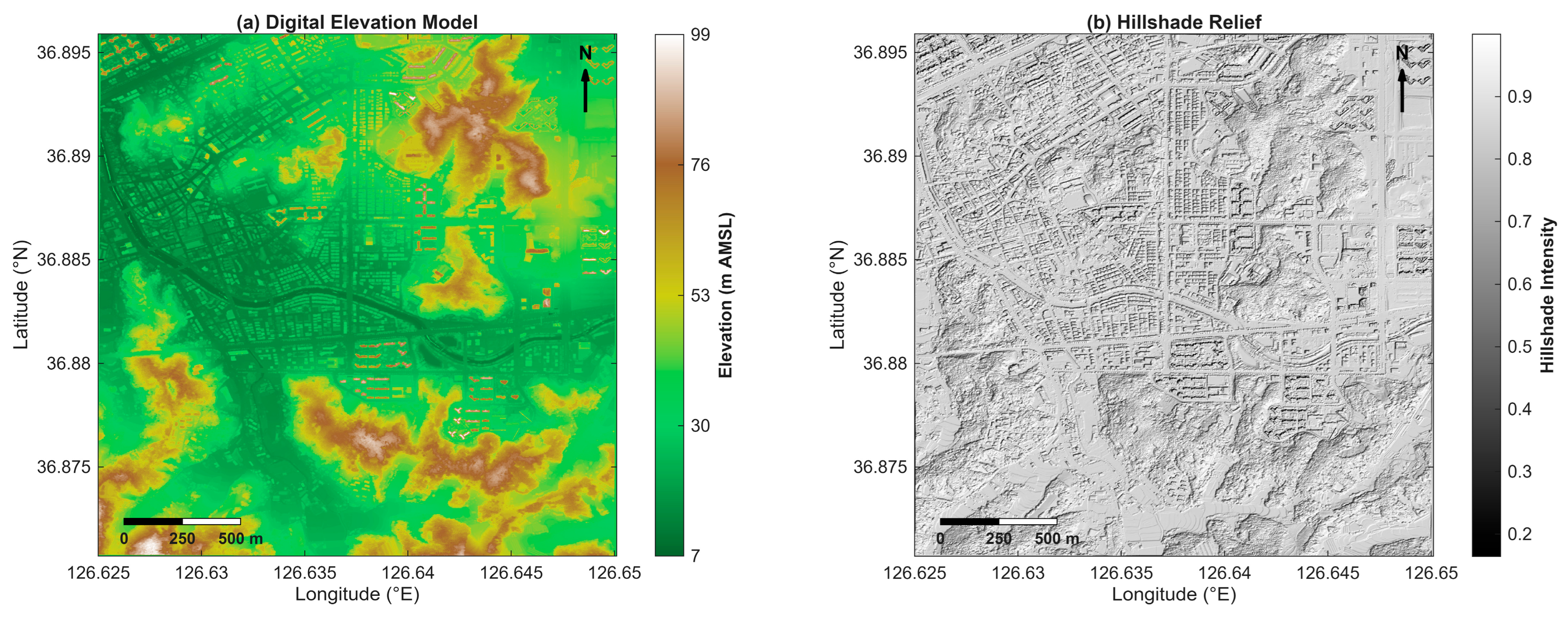
The study domain covers a 6.18 km² sub-area within Dangjin City (126.625–126.650° E, 36.875–36.895° N), delineated by the spatial extent of the airborne LiDAR survey (see Section 1.3 for city-level context). As shown in Figure 1a, the terrain is characteristic of a coastal plain-to-upland transition zone, with elevations ranging from approximately 10 m to 90 m above mean sea level and three broadly distinguishable physiographic units governing the spatial distribution of flood hazard. Low-lying coastal plains and river valleys below 20 m (dark green in Figure 1a) are concentrated along the central east–west river corridor and the western agricultural plains, characterised by gentle slopes of less than 2° and extensive paddy agriculture; these zones represent the area of highest flood exposure within the study domain. Transitional piedmont zones between 20 and 50 m exhibit moderate gradients of 2–8° with mixed residential and agricultural land use. Upland hills above 50 m (brown in Figure 1a), distributed across the northeastern and southwestern margins, have slopes exceeding 8° under predominantly forested cover and function as primary runoff-generating zones during extreme rainfall events.

The hillshade relief map (Figure 1b) reveals the micro-topographic complexity of the study domain at 1 m resolution, including drainage channels, road embankments, building footprints, and urban infrastructure networks that exert direct control over local flood pathways and inundation extent. The contrast between the densely developed urban fabric in the central zone and the irregular natural terrain of the surrounding uplands is clearly apparent, underscoring the importance of sub-metre topographic resolution for accurate flood boundary delineation. This topographic configuration produces a systematic downstream reduction in hydraulic gradient as rivers descend onto the coastal plain, suppressing flow velocity and promoting water ponding in topographic depressions. Gravitational drainage is further constrained by proximity to sea level, particularly during high-tide conditions when tidal backwater effects impede river discharge and extend inundation duration in the lowest-lying zones—a compound mechanism that distinguishes Dangjin’s flood regime from purely riverine systems [35].

Dangjin’s hydrological system comprises several interconnected river networks draining the surrounding upland areas and converging in the coastal lowlands before discharging into the Yellow Sea through three major tidal reservoirs—Sapgyoho, Seongmunho, and Daeho—each equipped with tidal sluice gates and pumping stations. The drainage network has been extensively modified through agricultural development and urbanisation, incorporating levees, pumping stations, and tide gates designed under historical precipitation regimes [3]. The 2024–2025 extreme events, producing cumulative totals of 214.6 mm and 377.4 mm respectively over short durations, are reported to have exceeded the operational thresholds of several of these structures, exposing a fundamental mismatch between existing design standards and the intensified precipitation regime emerging under contemporary climate conditions [1,4]. Dangjin’s co-location of major industrial complexes—including steel manufacturing, thermal power generation, and port infrastructure—with flood-prone agricultural lowlands means that inundation events can generate economic losses substantially exceeding direct physical damage, reinforcing the practical urgency of the high-resolution flood susceptibility framework developed in this study.

2.2. The 2024–2025 Extreme Rainfall Events

The catastrophic flooding that struck Dangjin City in July 2024 and July 2025 resulted from extreme monsoon precipitation events that exceeded regional historical records and overwhelmed both natural drainage systems and engineered flood-control infrastructure. Both events occurred within the East Asian summer monsoon season, during which quasi-stationary frontal boundaries, moisture convergence from the western North Pacific, and convective instability collectively generate intense and prolonged rainfall across the Korean Peninsula [36,37].

2.2.1. Meteorological Conditions

The first event, on 18 July 2024, developed under a quasi-stationary Changma frontal boundary established over the central Korean Peninsula, separating cooler continental air masses to the north from warm, moisture-laden maritime air advancing northward from the Yellow Sea. Strong low-level moisture flux along the western rim of the western North Pacific subtropical high (WNPSH) sustained convective precipitation cells that trained repeatedly over the same geographic sector—a mesoscale mechanism well documented for catastrophic frontal rainfall episodes in the region [36,37]. Peak hourly intensity reached 87.0 mm h⁻¹ at Dangjin, and although the most intense phase lasted approximately two to three hours, intermittent heavy rainfall persisted for 12–18 h, accumulating substantial totals across the catchment.

The 2025 event was more severe in both intensity and duration. A persistent monsoon depression stalled over central South Korea during July 2025, maintaining thermodynamic conditions favorable for repeated convective development over several consecutive days [36,38]. Maximum hourly intensities exceeded 110 mm h⁻¹, and Jeongmi-myeon in the southeastern portion of Dangjin City recorded a cumulative monthly total of approximately 454 mm—representing roughly 35–40% of mean annual precipitation concentrated within a single month and likely exceeding the 200-year return-period threshold based on regional intensity–duration–frequency statistics. Unlike the 2024 event, the multi-day structure of the 2025 episode allowed progressive soil saturation and groundwater rise between rainfall pulses, substantially amplifying surface runoff ratios during successive convective episodes and preventing effective inter-event drainage.

The 2024–2025 Dangjin extremes are consistent with a broader, regionally documented trend of intensifying East Asian monsoon rainfall. Observational analyses spanning 1958–2015 document a 17 ± 3% increase in East Asian summer monsoon frontal rainfall intensity, with climate model attribution indicating that anthropogenic greenhouse gas forcing contributed approximately 5.8% of that intensification through enhanced moisture transport and a strengthened WNPSH [36]. Detection–attribution studies further demonstrate a statistically discernible anthropogenic signal in both hourly- and daily-scale precipitation extremes across eastern China and the Korean Peninsula, with sub-daily extremes intensifying at rates approaching or exceeding Clausius–Clapeyron thermodynamic expectations of ~6–7% K⁻¹ [39,40]. High-resolution model projections under continued warming indicate that 99th-percentile monsoon precipitation may intensify at super-Clausius–Clapeyron rates of approximately 8% K⁻¹, particularly within Meiyu–Changma frontal bands [40,41]. The consecutive record-breaking monsoon seasons observed across East Asia in 2018, 2020, 2022, and 2024—each linked to anomalous moisture convergence, strengthened subtropical highs, and intraseasonal oscillation forcing—provide regional context for the exceptional intensity values recorded at Dangjin [36,38,42].

2.2.2. Flood Characteristics and Impacts

The extreme precipitation triggered compound flooding involving the simultaneous interaction of riverine overflow, pluvial inundation, and tidal backwater effects—a configuration consistent with the definition and documented dynamics of compound coastal–estuarine flood events, in which concurrent heavy rainfall, elevated river discharge, and tidal forcing mutually amplify inundation extent and duration [43,44,45]. Rivers rose rapidly during peak rainfall intensity, reaching stages that overtopped or breached levees at multiple locations along the main river corridors. Agricultural drainage networks, designed for normal-season conditions, became secondary conveyance pathways that propagated floodwater deep into low-lying agricultural and residential zones. In coastal and estuarine reaches, tidal backwater from the Yellow Sea suppressed gravity drainage and extended inundation well beyond the cessation of rainfall.

Inundation depths varied spatially in accordance with terrain position, proximity to overflow and breach locations, and local drainage capacity. The most severely affected areas recorded depths exceeding 2.0 m—consistent with the 2.0 m inundation scenario subsequently evaluated in this study (Section 3)—while more extensive areas experienced depths of 0.5–1.5 m, causing substantial structural damage and limiting emergency vehicle access. Temporal flood evolution also differed markedly by hydrological setting: flash flooding in upland tributary basins developed within one to two hours of peak rainfall intensity, whereas main-channel flooding along larger rivers evolved over six to twelve hours, permitting partial warning dissemination. Some low-lying areas remained inundated for three to seven days, complicating emergency operations and delaying systematic damage assessment.

Documented impacts spanned multiple sectors. Transportation networks were disrupted by road submersion, bridge damage from debris-laden high flows, and rail service suspension. Critical infrastructure—including electrical substations, water treatment facilities, and telecommunications systems—sustained service interruptions extending days to weeks beyond the initial inundation. Agricultural losses were severe, with rice paddies at critical growth stages, greenhouse operations, and livestock facilities sustaining direct damage from inundation, soil contamination, and associated pathogen exposure. The recurrence of major flooding in consecutive years under intensifying monsoon precipitation directly motivates the high-resolution geospatial risk assessment framework developed in this study.

2.3. Data Acquisition and Preprocessing

2.3.1. High-Resolution LiDAR Data

The topographic foundation of this study is a 1 m resolution airborne LiDAR-derived Digital Elevation Model (DEM) produced under South Korea’s national topographic mapping program administered by the National Geographic Information Institute (NGII). The DEM covers the entire administrative area of Dangjin City and meets the NGII national standard for vertical accuracy, with a root mean square error (RMSE) of 0.25 m or better [46]. The dataset was generated from airborne laser scanning acquisitions using multiple overlapping flight lines to ensure complete coverage and minimize occlusion effects in complex terrain.

Raw point cloud preprocessing followed a standard classification workflow to isolate bare-earth ground returns from non-ground features including buildings, vegetation, vehicles, and utility structures. Classification employed an adaptive triangulated irregular network (TIN) algorithm applied iteratively to progressively refine ground-point identification, with manual correction applied in densely built urban blocks where automated classification is prone to commission errors [8,18]. Only points assigned to the ground class were retained for subsequent DEM generation. Continuous raster surfaces were produced by TIN interpolation of classified ground points followed by conversion to a 1 m grid, preserving measured elevation values at control points while generating smooth interpolated surfaces in inter-point intervals.

Quality control included independent validation against surveyed ground control points distributed across terrain types to confirm compliance with the NGII vertical accuracy standard. Hillshade and slope derivative maps were inspected visually to identify and correct residual artifacts from vegetation filtering errors or tile-boundary mismatch. The quality-controlled 1 m DEM captures micro-topographic features critical for hydrological analysis, including shallow depressions, field drainage ditches, road embankments, and channel margins that are unresolvable at the coarser resolutions of globally available DEMs such as SRTM (30 m) or ASTER GDEM (30 m) [11,30].

2.3.2. Flood Inventory Mapping

A multi-source flood inventory was compiled to document inundation extent during the July 2024 and July 2025 events, providing the observational basis for model validation. The primary spatial data source was Sentinel-1 C-band SAR imagery acquired by the European Space Agency’s Copernicus programme. SAR-based change detection was performed by comparing backscatter intensity images acquired during flood conditions against pre-event reference composites; inundated surfaces were identified by their characteristically low backscatter signal relative to dry-land baselines, a widely applied methodology for rapid flood extent mapping [47,48]. Where cloud-free conditions permitted, optical imagery from Sentinel-2 MultiSpectral Instrument was analyzed using the Modified Normalized Difference Water Index (MNDWI) to corroborate SAR-derived flood boundaries.

SAR- and optical-derived extents were supplemented by post-event field records from emergency management agencies, including GPS-surveyed high-water marks, debris deposition lines, and structural damage assessments. Government damage reports from Dangjin City and Chungcheongnam-do Province provided georeferenced information on flooded road segments, inundated buildings, and declared evacuation zones. All source layers were integrated in a GIS overlay framework; areas identified as flooded by two or more independent sources were classified as confirmed inundation, while single-source identifications were assigned probable inundation status. For quantitative model validation, only confirmed inundation areas were used; probable areas informed qualitative interpretation only.

The confirmed flood inventory ultimately comprises nine georeferenced points (four from the July 2024 event; five from the July 2025 event). This limited count reflects the stringent multi-source confirmation criterion: only locations independently identified as flooded by two or more data sources were retained, while numerous single-source identifications were excluded to minimise false-positive contamination. Point coordinates were assigned from field reconnaissance GPS waypoints and administrative damage record addresses geocoded to building or parcel centroids, rather than from precision RTK-GPS surveys or pixel-level remote sensing classification, introducing estimated positional uncertainties of 50–150 m. These uncertainties motivated the adoption of the buffer-based validation approach described in Section 2.5.5, rather than direct point-in-polygon assessment.

2.3.3. Ancillary Geospatial Data

Several additional datasets were incorporated to support flood susceptibility analysis and contextual interpretation. Hourly precipitation records from the Korea Meteorological Administration (KMA) Automatic Weather Station (AWS) network provided rainfall intensity and cumulative totals for the 2024 and 2025 flood events at stations within and adjacent to the study area, serving as the primary meteorological basis for flood inventory compilation and scenario depth selection. Land use and land cover data from the national land cover map (Ministry of Environment, 1:5000 scale) were used to characterise surface conditions and interpret spatial patterns of runoff generation across the study domain. The river and drainage network was extracted from the 1 m DEM using flow direction and flow accumulation algorithms and subsequently verified against the national hydrographic database (NGII 1:5000 stream layer) to ensure topological consistency with the terrain-derived drainage structure. All datasets were projected to the Korean Geodetic Datum 2000 (KGD2000) coordinate system, UTM Zone 52N projection, and resampled or rasterised to match the 1 m DEM grid prior to analysis.

2.4. Topographic Analysis and Feature Extraction

2.4.1. Digital Elevation Model Generation

The 1 m resolution LiDAR-derived DEM described in Section 2.3.1 served as the primary topographic input for all subsequent analyses. Prior to parameter extraction, the raw point cloud was preprocessed by removing elevation outliers exceeding three standard deviations from the local mean, followed by Gaussian smoothing (σ = 1 pixel) to suppress high-frequency noise while preserving hydrologically significant micro-topographic features. Residual data voids were filled using a moving-mean interpolation algorithm. Hydrological conditioning was applied by filling spurious depressions using a priority-flood algorithm, ensuring topological continuity of the drainage network. Flow direction was subsequently assigned using the deterministic eight-direction (D8) routing algorithm [49], which partitions the contributing area to a single downslope neighbor and underpins all flow-accumulation computations. Hillshade maps (azimuth 315°, altitude 45°) were generated as a visual quality-assurance layer to verify the absence of systematic artifacts across the 6.18 km² study extent.

2.4.2. Derived Terrain and Hydrological Parameters

Five terrain and hydrological parameters were extracted from the preprocessed DEM and normalized to the range [0, 1] prior to index computation (

Table 1. Terrain and hydrological parameters used in the Flood Susceptibility Index (FSI) computation, with physical rationale, normalization direction, and assigned weights.

Parameter	Physical Rationale	Normalization	Weight
Elevation	Low elevation → greater flood exposure	Inverted	0.20
Slope	Gentle slope → water ponding	Inverted	0.30
TWI	High TWI → water accumulation	Direct	0.25
Flow accumulation	High accumulation → channel proximity	Direct	0.15
Distance to stream	Short distance → overflow exposure	Inverted	0.10
Total			1

). Parameters for which low values indicate greater flood exposure were inverted during normalization so that higher normalized scores consistently denote higher flood susceptibility.

Elevation represents the primary gravitational control on flood inundation; lower-lying areas are more prone to surface water accumulation and receive inverted normalization (weight = 0.20).

Slope, computed in degrees using finite-difference gradient operators, governs the partitioning of rainfall between infiltration and surface runoff. Gentle slopes (<2–3°) promote water ponding, while steeper gradients (>8–10°) accelerate drainage toward receiving channels. Slope is inverted so that flat terrain scores highest (weight = 0.30).

Topographic Wetness Index (TWI) quantifies the tendency of a grid cell to accumulate soil moisture and is defined as (weight = 0.25):

$$\mathrm{TWI}=\ln \left({\displaystyle \frac{a}{\tan \mathsf{\beta }}}\right)$$

(1)

Flow accumulation, derived from D8 routing and log-transformed as $\mathrm{l}\mathrm{n}(\mathrm{flow}+1)$ to reduce right-skew, indicates the upstream drainage area contributing runoff to each cell and serves as a proxy for channel network position. Direct normalization is applied (weight = 0.15).

Distance to the nearest stream was computed as the Euclidean distance from each cell to the extracted channel network, defined by the 95th-percentile threshold of log-transformed flow accumulation. Proximity to streams elevates flood exposure; accordingly, the parameter is inverted (weight = 0.15).

The relative weights in Table 1 were informed by the parameter importance rankings identified in refs. [29,50], and adjusted for the low-gradient coastal-plain characteristics of the Dangjin study area. The elevated weight assigned to slope (0.30) reflects its dominant role in partitioning rainfall between infiltration and surface runoff in terrain where micro-topographic gradient variations of less than 2° govern the spatial extent of water ponding across agricultural lowlands.

The five-parameter configuration was deliberately restricted to terrain attributes extractable from the LiDAR DEM alone, ensuring that the framework remains deployable in municipalities where ancillary thematic datasets are unavailable or maintained at incompatible resolutions. Four additional conditioning factors commonly discussed in the flood susceptibility literature were considered but excluded for the following reasons. Land use and land cover data, although available from the national land cover map (Ministry of Environment, 1:5000 scale; Section 2.3.3), were used only for contextual interpretation because classification schemes and update cycles vary across municipalities, undermining cross-site reproducibility; moreover, within the Dangjin study domain, the dominant land covers—paddy agriculture and low-density residential development—exhibit relatively homogeneous hydrological behaviour compared with the pronounced topographic variability resolved at 1 m. Spatially distributed soil hydraulic properties (saturated conductivity, porosity) are published by the Rural Development Administration at 1:25,000 scale with polygon-based taxonomic units that would introduce artificial discontinuities on a 1 m grid; furthermore, during the extreme rainfall intensities recorded in 2024 (87.0 mm h⁻¹) and 2025 (>110 mm h⁻¹), infiltration capacity is rapidly exceeded across all local soil types, and flood extent becomes governed primarily by topographic routing. Engineered stormwater drainage specifications (pipe diameter, gradient, inlet spacing, pump capacity) are not maintained in GIS-ready formats by Dangjin City, precluding their systematic incorporation. Rainfall intensity was intentionally excluded from the FSI to preserve the index as a time-invariant susceptibility surface; event-specific precipitation magnitude is instead represented through the scenario-based inundation component (Section 2.5.4), where the three depth thresholds (Δh = 0.5, 1.0, 2.0 m) implicitly correspond to increasing rainfall severity. This separation between static terrain-based susceptibility and event-driven hazard magnitude follows established multi-criteria flood assessment practice [29]. The implications of the topography-only parameter set for transferability to urbanised or geologically heterogeneous settings are discussed in Section 4.3.

2.4.3. Spatial Distribution of Representative Terrain Parameters

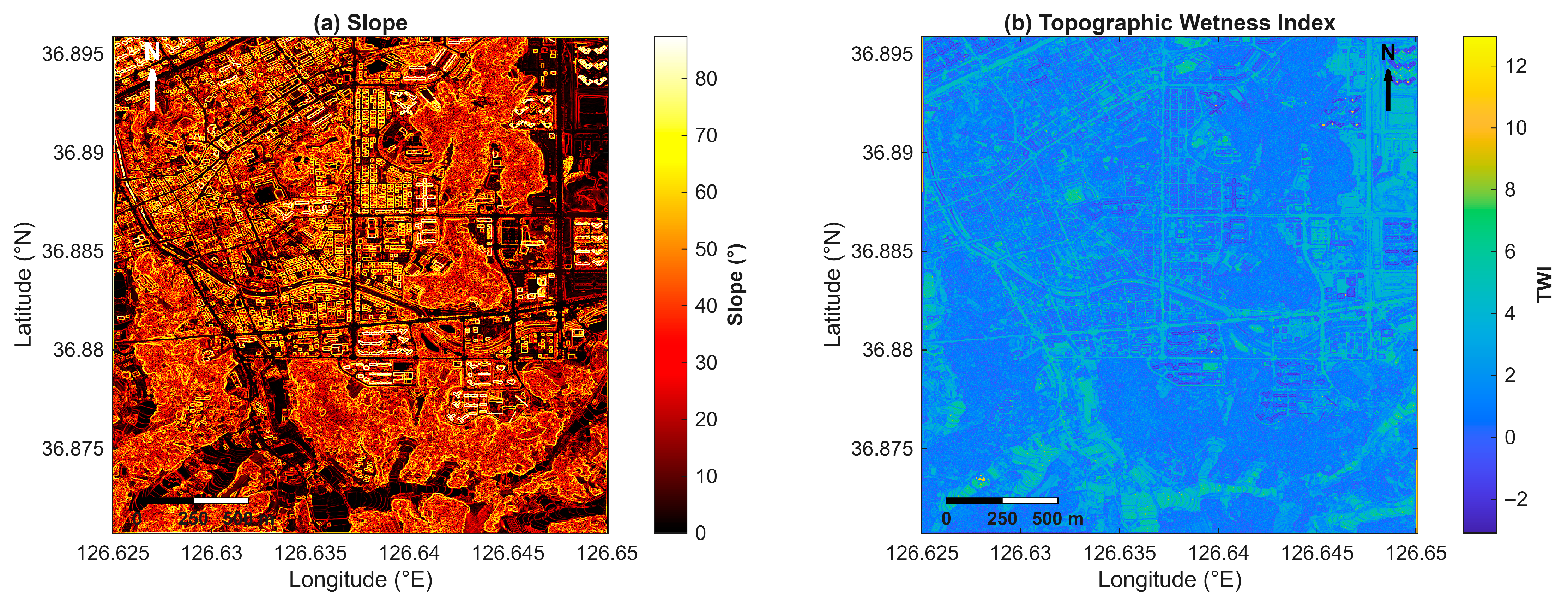
Figure 2 illustrates the spatial distribution of two representative parameters across Dangjin City: (a) slope and (b) TWI. Slope values exceeding 40° (red–yellow tones) are concentrated in the dense urban core and along engineered embankments, whereas agricultural lowlands and tidal flats exhibit slopes consistently below 5° (dark brown–black tones), confirming the dominance of low-gradient terrain most susceptible to surface ponding. TWI values range from near zero (blue, built-up areas with divergent flow paths) to above 8 (green–yellow, river corridors and peripheral low-lying depressions), spatially delineating the principal zones of moisture convergence. Together, these two indices capture the contrasting flood-generating mechanisms operative in Dangjin: rapid urban runoff on impervious surfaces and prolonged inundation in flat agricultural and estuarine zones, both of which are further quantified through the composite Flood Susceptibility Index derived in Section 3.

2.5. Methodological Framework

2.5.1. Overall Workflow

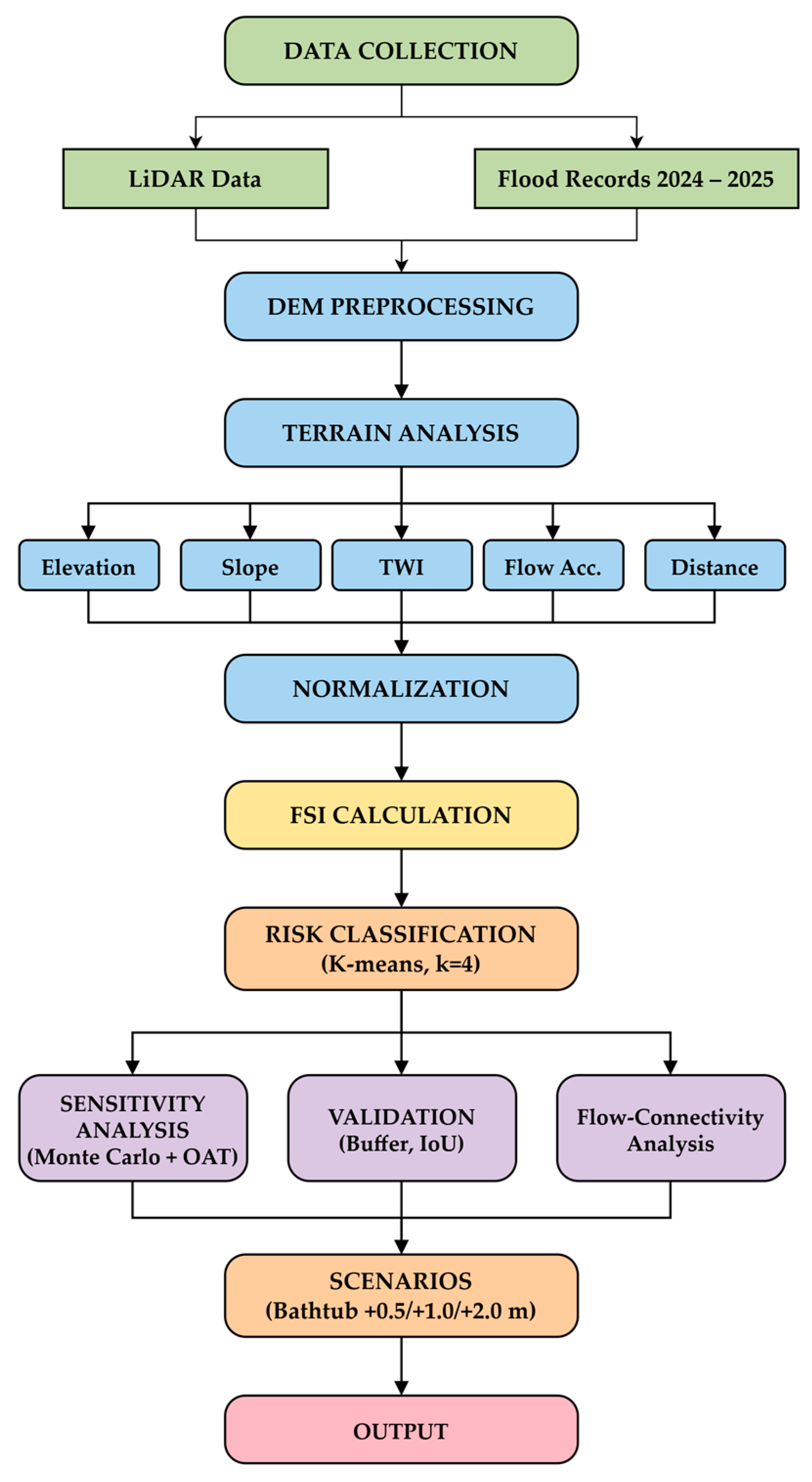
The analytical framework integrates LiDAR-derived terrain analysis, multi-parameter Flood Susceptibility Index (FSI) computation, unsupervised risk classification, scenario-based inundation mapping, and inventory-based validation into a sequential geospatial workflow. The complete processing chain is illustrated in Figure 3. Input data comprise two independent streams: (i) airborne LiDAR point-cloud data processed into a 1 m DEM (Section 2.3.1), and (ii) the 2024–2025 flood inventory compiled from Sentinel-1 SAR imagery, field surveys, and government damage reports (Section 2.3.2). These two data streams serve distinct roles throughout the framework—the LiDAR DEM drives all terrain analysis and susceptibility computations, while the flood inventory is reserved exclusively for independent validation and is not used during model development, thereby preventing circular assessment. The full workflow was implemented in MATLAB R2025b and applied at 1 m resolution across the 6.18 km² study domain.

2.5.2. Flood Susceptibility Index Computation

The FSI was computed as a weighted linear combination of the five normalized terrain parameters described in Section 2.4:

$$\mathrm{F}\mathrm{S}\mathrm{I}=0.20\cdot \widehat{\mathrm{E}}+0.30\cdot \widehat{\mathrm{S}}+0.25\cdot \widehat{\mathrm{T}}+0.15\cdot \widehat{\mathrm{F}}+0.10\cdot \widehat{\mathrm{D}}$$

(2)

where $\widehat{E}$, $\widehat{S}$, $\widehat{T}$, $\widehat{F}$ and $\widehat{D}$ denote the (inverted where applicable) values of elevation, slope, TWI, flow accumulation, and distance to stream, respectively. The parameter weights were informed by the importance rankings identified in systematic reviews of GIS-based flood susceptibility studies [29,50], as described in Section 2.4.2.

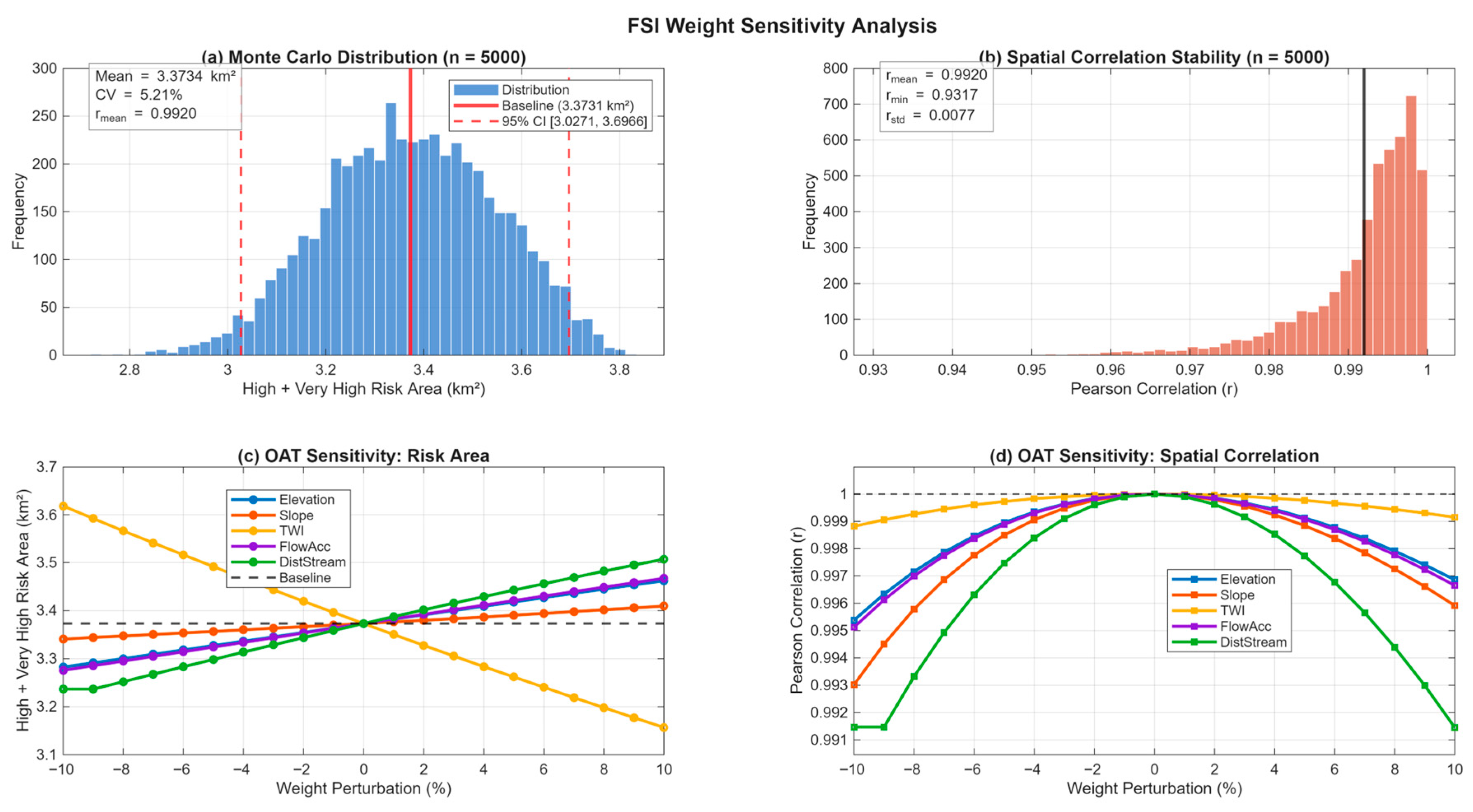
To assess the robustness of the literature-derived weight vector, a Monte Carlo sensitivity analysis was performed. In each of 5000 realisations, each of the five baseline weights was independently perturbed by a random value drawn from a uniform distribution over the interval [−0.10, +0.10]. The perturbed weight vector was then normalised to unit sum to maintain the linear combination constraint. For each realisation, the FSI was recomputed across the full study domain and classified into four risk levels using the k-means-derived thresholds established from the baseline configuration (FSI = 0.489, 0.631, 0.767); the combined High + Very High risk area was then recorded. Additionally, a one-at-a-time (OAT) analysis was conducted in which each individual weight was varied from −0.10 to +0.10 of its baseline value (in increments of 0.01) while holding all other weights at their baseline values and renormalising, to identify the relative influence of each parameter on the high-risk extent. Spatial agreement between the baseline and perturbed FSI surfaces was quantified using Pearson’s correlation coefficient (r).

2.5.3. K-Means Risk Classification

The continuous FSI surface was classified into four discrete flood risk categories—Very High, High, Moderate, and Low—using K-means clustering (k = 4, five independent replicates with random initialization). Clusters were reordered by ascending mean FSI value to ensure consistent class labelling across replicates. This unsupervised approach avoids subjective threshold selection and allows class boundaries to emerge from the natural structure of the data [29,51].

2.5.4. Scenario-Based Inundation Mapping

To complement the FSI-based susceptibility analysis, four static inundation scenarios were generated by identifying all DEM cells with elevation at or below a scenario-specific water surface defined as:

$$h_{\mathrm{scenario}}=h_{\mathrm{base}}+\mathsf{\Delta }h$$

(3)

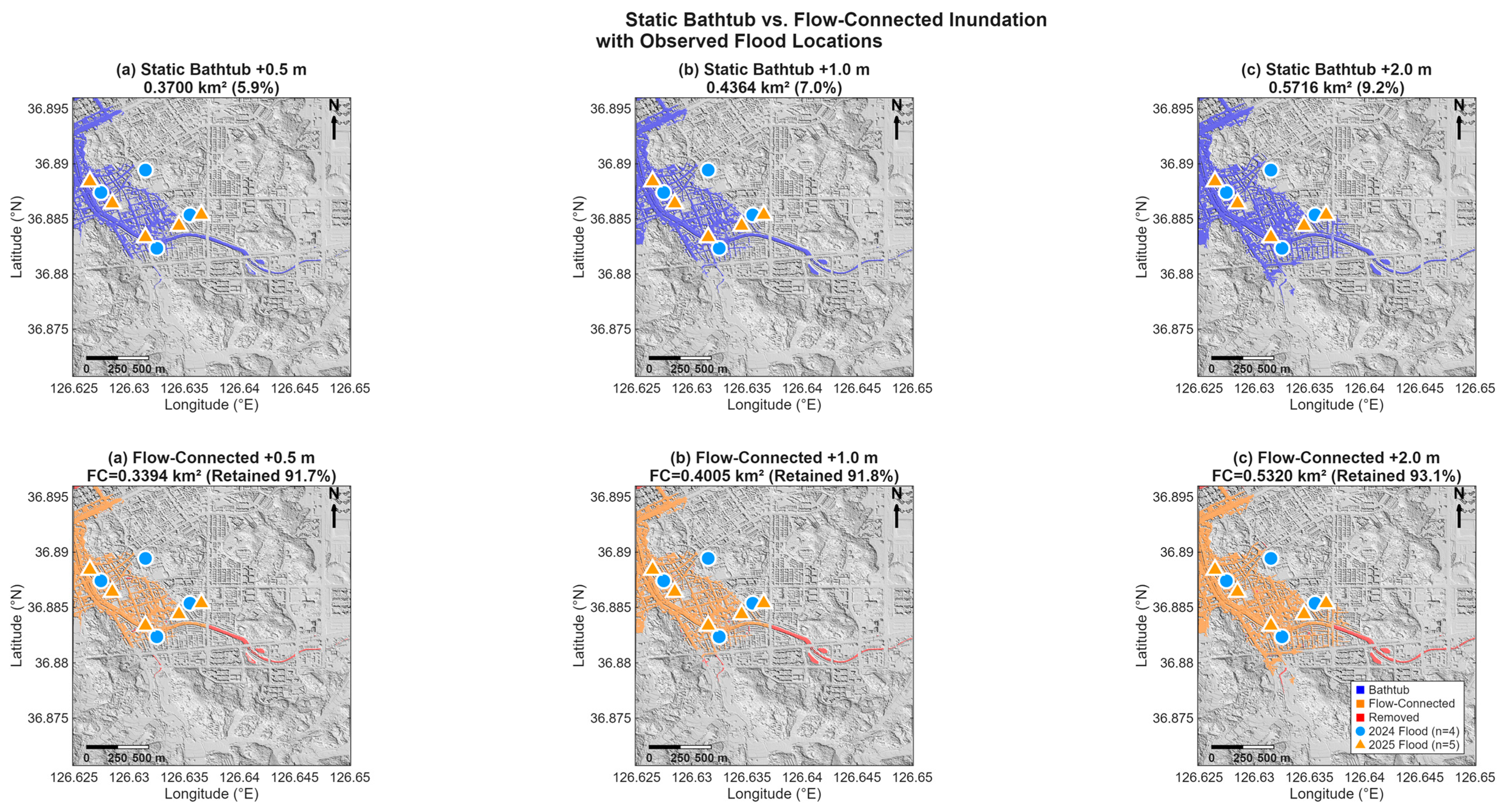
where h_base corresponds to the 5th-percentile elevation of the DEM within the analysis domain and Δh ∈ {0.5, 1.0, 2.0} m represents incremental flood depth thresholds corresponding to minor, moderate, and severe inundation conditions, respectively. The 5th-percentile elevation (h_base = 13.29 m AMSL) was selected as the baseline water-level proxy for three reasons: (i) it approximates the elevation of the lowest-lying channel thalweg and adjacent floodplain margins within the study domain, where water accumulates first during rising flood stages; (ii) it is consistent with the Height Above Nearest Drainage (HAND) concept, in which relative elevation above the local drainage network serves as a first-order predictor of inundation exposure [52]; and (iii) it provides an objective, reproducible threshold that does not require observed stage–discharge records or tidal gauge data, maintaining the data-limited constraint of the overall framework. To evaluate the sensitivity of this choice, inundation extents were also computed using the 1st-percentile (10.73 m) and 10th-percentile (15.64 m) DEM elevations as alternative baselines. At the +2.0 m scenario, the resulting flooded areas were 0.25 km² (1st percentile), 0.57 km² (5th percentile), and 0.89 km² (10th percentile). The substantial variation reflects the physical difference between the three reference surfaces: the 1st-percentile baseline confines inundation to the deepest channel incisions, whereas the 10th-percentile baseline extends it onto higher floodplain margins. The 5th-percentile value captures the transition between confined channel flooding and broader floodplain inundation, and its scenario outputs (0.37–0.57 km² across the three depth increments) are consistent with the observed flood damage locations from the July 2024 and July 2025 events. A flow-connectivity analysis using morphological reconstruction from the D8-derived stream network refs [49,53] further confirmed that 91.7–93.1% of the bathtub-predicted inundation area is hydraulically connected to the drainage network (Appendix A Figure A1). This bathtub approach provides first-order spatial estimates of inundation extent without requiring dynamic hydraulic simulation, and is appropriate for planning-level risk mapping where detailed channel bathymetry and roughness data are unavailable [35,54].

2.5.5. Inventory-Based Validation

Model accuracy was evaluated against the independently compiled 2024–2025 flood inventory (Section 2.3.2). For each observed flood point, circular buffers of 100, 200, and 300 m radius were generated, and the proportion of buffer area classified as High or Very High risk was computed. Two metrics were reported: spatial accuracy (percentage of buffer area in high-risk class) and Intersection over Union (IoU), defined as:

$$\mathrm{IoU}={\displaystyle \frac{\left(B_{2024}\cup B_{2025}\right)\cup R_{\mathit{high}}}{\left(B_{2024}\cup B_{2025}\right)\cap R_{\mathrm{high}}}}\times 100\%$$

(4)

where $B_{2024}$, $B_{2025}$ denote the union of buffer polygons for each event and $R_{\mathrm{high}}$ denotes the High + Very High risk raster. These metrics provide a spatially explicit, threshold-independent measure of model skill consistent with flood susceptibility validation practice [47,48].

3. Results

3.1. Flood Risk Classification

3.1.1. FSI Computation and K-Means Classification

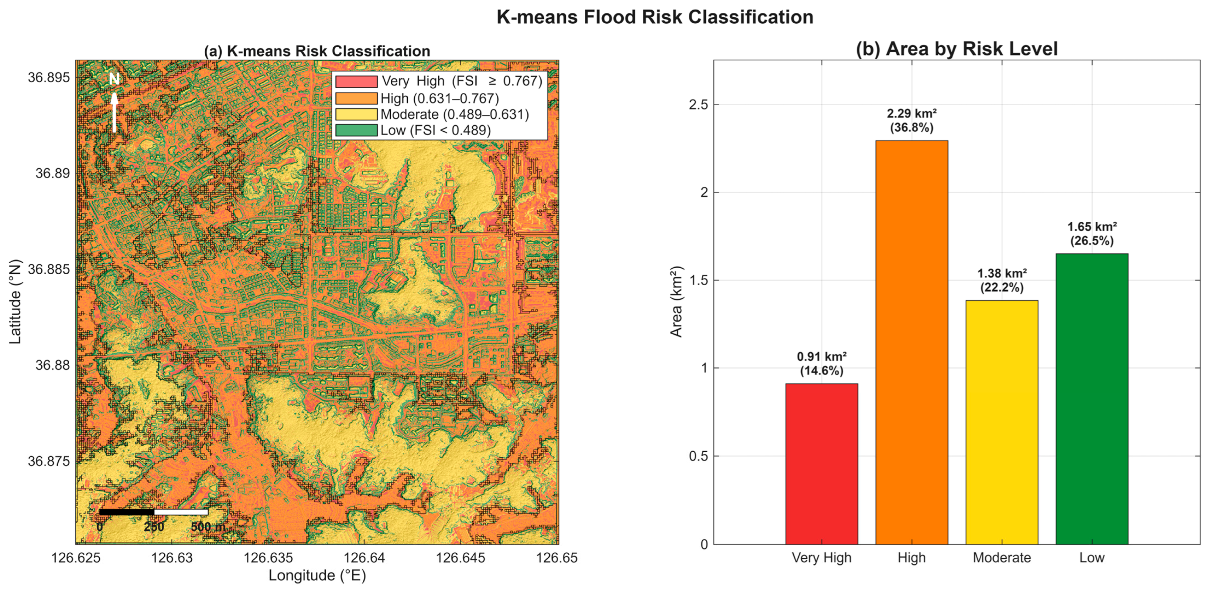
The Flood Susceptibility Index (FSI) computed from the five weighted terrain parameters (Section 2.5.2) was applied across the LiDAR analysis domain (36.875–36.895° N, 126.625–126.650° E; total area ≈ 6.18 km²). K-means clustering (k = 4, five independent replicates) partitioned the continuous FSI surface into four discrete risk classes reordered by ascending cluster mean FSI. The resulting classification map and corresponding areal statistics are presented in Figure 4 and

Table 2. Flood risk classification statistics derived from K-means clustering of the FSI surface.

Risk Class	Area (km2)	% of Analysis Area
Very High	0.87	14.1
High	2.30	37.2
Moderate	1.63	26.4
Low	1.38	22.3
Total	6.18	100

, respectively.

The High Risk class dominates the analysis area at 37.2%, reflecting the extensive low-gradient coastal plain in the western portion of the domain. The combined High and Very High Risk classes account for 3.17 km² (51.3% of the analysis area), confirming that more than half of the mapped domain carries substantial flood susceptibility under the terrain-based FSI framework.

3.1.2. Spatial Distribution by Risk Class

The spatial pattern in Figure 4a reveals a clear west–east susceptibility gradient consistent with the macro-topographic structure described in Section 2.1. The Very High Risk class (red, 0.87 km²) is confined to valley floors and river channel margins in the southwestern sector, where TWI exceeds 8, slope falls below 2°, and elevation falls below 15 m AMSL. The High Risk class (orange, 2.30 km²) forms a near-continuous sheet across the central and western agricultural lowlands, spatially coinciding with the TWI > 6 zones illustrated in Figure 2b. The Moderate Risk class (yellow, 1.63 km²) forms a transitional envelope along the urban–agricultural boundary, where fine-scale terrain relief from road embankments introduces localised FSI departures. The Low Risk class (green, 1.38 km²) is concentrated in the northeastern upland patches where slopes exceed 8° (Figure 2a) and TWI remains below 3 (Figure 2b). The combined High and Very High Risk extent of 3.17 km² encompasses the principal 2024–2025 inundation locations, providing the spatial basis for the validation analysis in Section 3.3.

3.1.3. Sensitivity of FSI Classification to Weight Perturbation

A Monte Carlo sensitivity analysis (n = 5000; ±0.10 uniform weight perturbation) yielded a mean combined High + Very High risk area of 3.37 ± 0.18 km² (baseline: 3.37 km²), with a coefficient of variation of 5.21% and a 95% confidence interval of [3.03, 3.70] km². The mean Pearson correlation between perturbed and baseline FSI surfaces was r = 0.992 (min = 0.932), confirming strong spatial consistency. The one-at-a-time analysis identified TWI as the most influential parameter (area range = 0.46 km²), while slope—despite carrying the highest weight (0.30)—exhibited the smallest sensitivity (0.07 km²). Full results are presented in Appendix A Figure A2, and their implications for weight transferability are discussed in Section 4.3.

3.2. Scenario-Based Flood Inundation Mapping

3.2.1. Inundation Extent Across Three Depth Scenarios

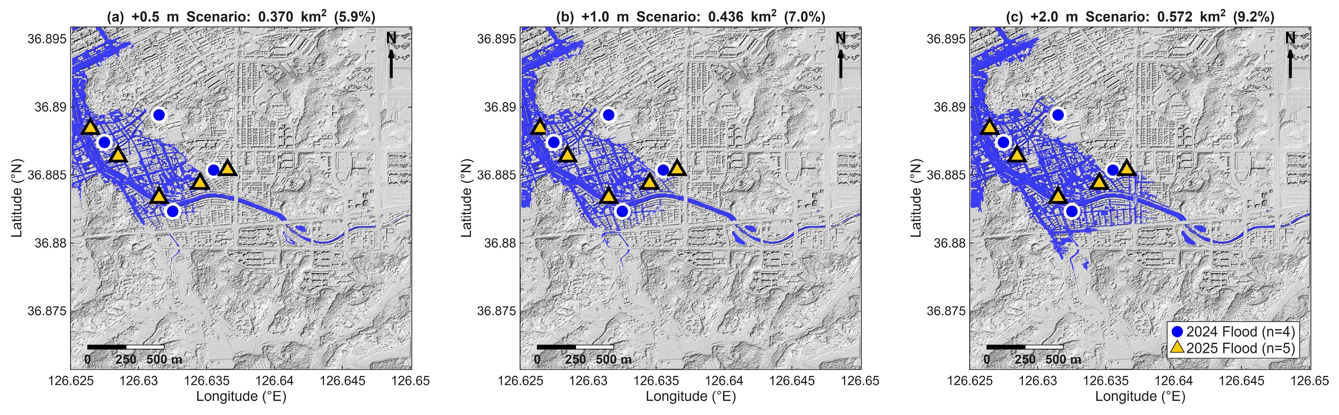
Static inundation scenarios were generated for three incremental depth thresholds above the DEM 5th-percentile baseline water level (h_base = 13.29 m AMSL), following the bathtub approach described in Section 2.5.4. The corresponding scenario water-surface elevations are 13.79 m (+0.5 m), 14.29 m (+1.0 m), and 15.29 m (+2.0 m) AMSL. The resulting inundation extents are mapped in Figure 5 alongside the confirmed 2024 and 2025 flood inventory points, and areal statistics are summarised in

Table 3. Simulated inundation area by flood depth scenario.

Scenario (Δh)	Inundated Area (km2)	% of Analysis Area	Incremental Increase (km2)
+0.5 m	0.370	5.9	—
+1.0 m	0.436	7.0	+0.066
+2.0 m	0.572	9.2	+0.136

.

The 0.5 m scenario (Figure 5a) delineates the narrowest inundation footprint of 0.370 km² (5.9% of the analysis domain), confined primarily to the main river channel corridor and its immediate margins. At this threshold, inundation follows a linear, channel-parallel pattern oriented northwest–southeast across the study domain. Two of the four 2024 flood inventory points (blue circles) fall within or immediately adjacent to this boundary, consistent with field-reported inundation depths of 0.5–1.0 m in the lower-lying channel proximal zones during the July 2024 event (Section 2.2).

The 1.0 m scenario (Figure 5b) expands the inundated area to 0.436 km² (7.0%), an incremental increase of 0.066 km² relative to the 0.5 m threshold. Lateral spreading from the main channel into adjacent low-lying agricultural and peri-urban areas becomes apparent, particularly in the northwestern sector of the study domain where flat terrain (slope < 2°) offers minimal resistance to lateral inundation. The majority of the 2025 flood inventory points (yellow triangles) are captured within the 1.0 m inundation boundary, suggesting that the hydraulic conditions during the July 2025 event corresponded broadly to a 1.0–2.0 m water level rise above baseline channel stage.

The 2.0 m scenario (Figure 5c) produces the largest simulated extent at 0.572 km² (9.2%), with an additional 0.136 km² relative to the 1.0 m threshold. At this depth, inundation extends across the full floodplain width in the northwestern lowland zone and connects previously isolated depressions within the urban-agricultural transition area through a network of drainage pathways resolved at 1 m DEM resolution. Nearly all observed flood inventory points from both 2024 and 2025 events fall within the 2.0 m inundation boundary, corroborating the field-reported maximum depths exceeding 2.0 m in the most severely affected locations (Section 2.2.2).

The non-linear area increment between the 1.0 m and 2.0 m scenarios (0.136 km² versus 0.066 km² for the 0.5–1.0 m step) reflects the progressive hydraulic connectivity of shallow topographic depressions that become inundated only at higher water levels, a behaviour characteristic of the low-gradient coastal plain terrain described in Section 2.1. A supplementary flow-connectivity analysis (Appendix A, Figure A1) confirmed that 91.7–93.1% of the bathtub-predicted inundation area is hydraulically connected to the D8-derived stream network, with disconnected cells confined to minor hillslope depressions that would not receive floodwater through surface or subsurface flow paths. The high retention rates are consistent with the dominant pluvial flooding mechanism in Dangjin, where sewer surcharge and manhole overflow during extreme rainfall distribute floodwater through the interconnected subsurface drainage network into topographically connected low-lying areas.

3.2.2. Inundation Depth Distribution and Spatial Correspondence with Observed Flood Inventory

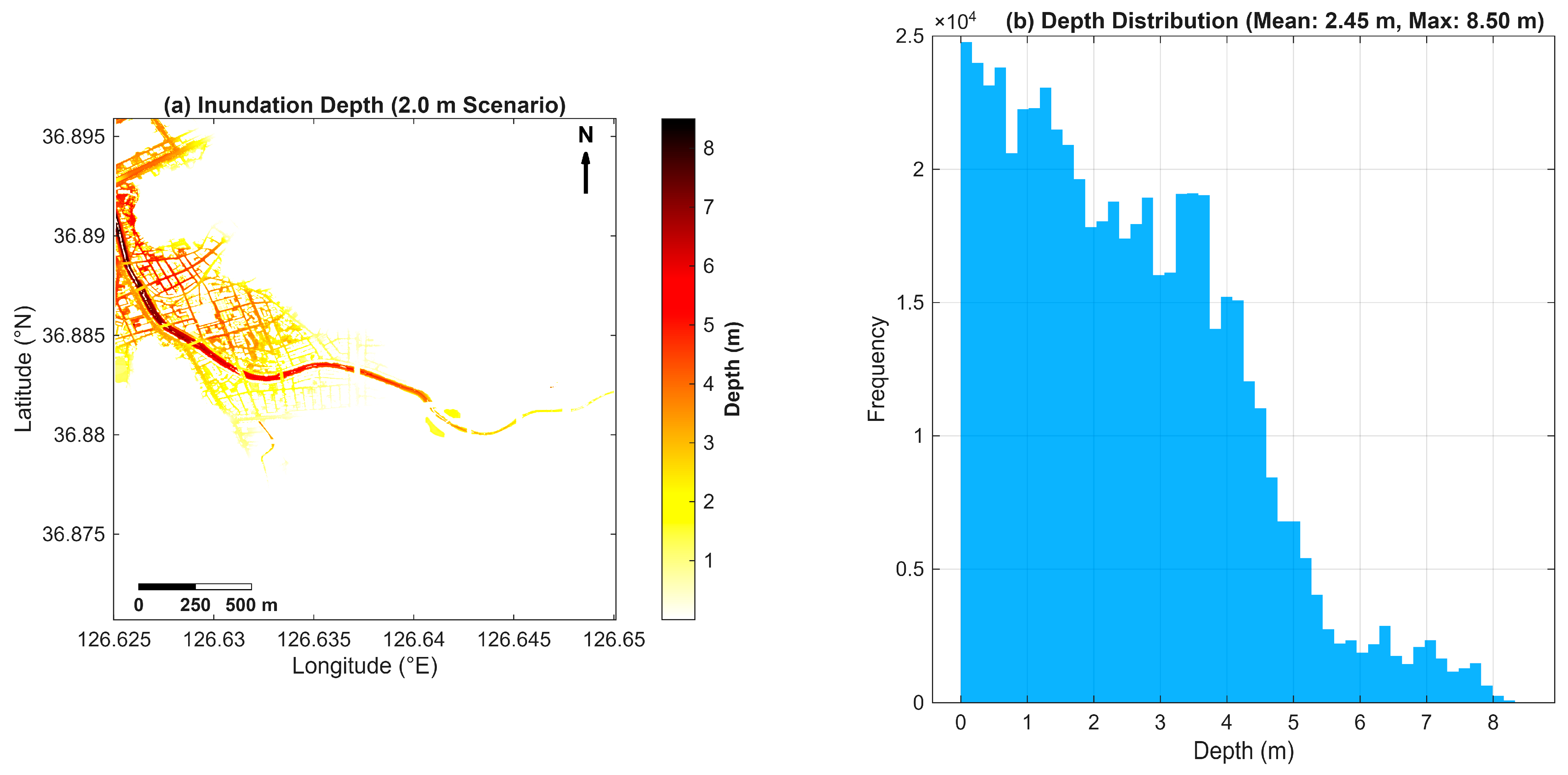
The spatial distribution of inundation depth under the 2.0 m scenario is presented in Figure 6a, with the corresponding frequency histogram shown in Figure 6b. Depth values across all flooded cells range from near zero at the inundation boundary to a maximum of 8.50 m along the principal river thalweg, with a domain mean of 2.45 m. The depth histogram (Figure 6b) exhibits a pronounced right-skewed distribution: the modal class corresponds to depths of 0–1 m, representing shallow floodplain-margin inundation where the water surface elevation marginally exceeds the DEM 5th-percentile baseline, while the extended right tail to 8.50 m reflects deeply incised channel sections where substantial water volume accumulates under the static bathtub assumption. A secondary frequency elevation is visible near the 3–4 m bin, corresponding spatially to the semi-confined channel reach in the northwestern sector where flow convergence amplifies local depth. The isolated single-cell artefact visible at approximately 36.875° N, 126.635° E in Figure 6a is excluded from all depth statistics.

The spatial overlay of simulated inundation extents with the 2024–2025 flood inventory points (Figure 5) reveals a progressive improvement in observed flood point capture as scenario depth increases. Under the 0.5 m scenario, 2 of 4 confirmed 2024 flood points (50%) and 2 of 5 confirmed 2025 flood points (40%) fall within the simulated inundation boundary, reflecting the localised, channel-proximal character of the lower-magnitude 2024 event. At the 1.0 m threshold, capture rates increase to 75% (3/4) for 2024 points and 80% (4/5) for 2025 points as lateral inundation expands into the northwestern lowland zone. The 2.0 m scenario achieves complete capture of all nine inventory points (100%), consistent with field-reported maximum inundation depths exceeding 2.0 m during the July 2025 event (Section 2.2). This spatial correspondence between scenario inundation boundaries and confirmed flood locations provides qualitative validation of the bathtub simulation approach and directly supports the quantitative buffer-based accuracy metrics reported in Section 3.3 [35,54].

3.3. Spatial Validation of the Flood Susceptibility Model

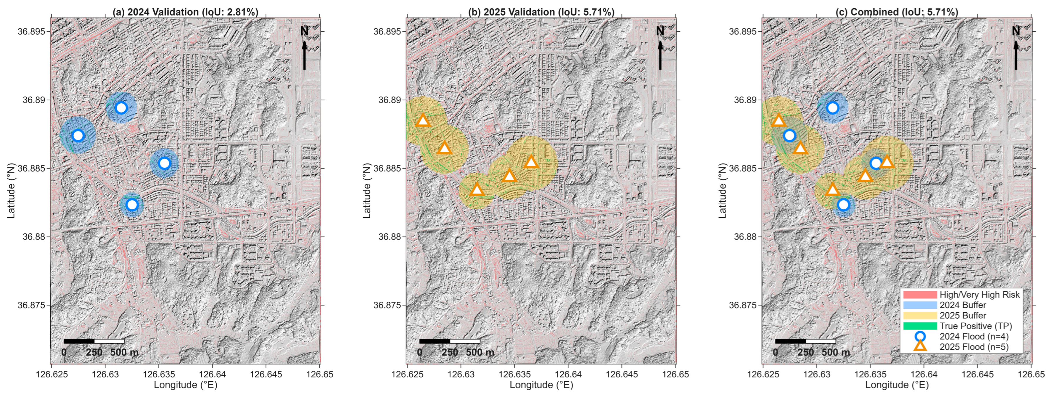
Spatial validation was performed by overlaying the modelled high-risk zones (FSI ≥ 95th percentile; 0.3119 km², 5.00% of the 6.18 km² study domain) against georeferenced flood inventory points from the July 2024 (n = 4; cumulative rainfall 214.6 mm) and July 2025 (n = 5; cumulative rainfall 377.4 mm) events. Buffer Accuracy and Intersection over Union (IoU) were computed for each event and for the combined inventory as defined in Section 2.5.3; results are summarised in

Table 4. Spatial validation metrics from buffer-overlap analysis of the 2024 and 2025 flood inventories against the modelled high-risk zone (FSI ≥ 95th percentile; 0.3119 km², 5.00% of study domain).

Metric	2024	2025	Combined
Buffer Accuracy (%)	8.23	9.96	9.50
IoU (%)	3.33	6.50	6.51
High-risk Area within Buffer (km2)	0.0165	0.0491	0.0535
High-risk Coverage (%)	5.29	15.74	17.14

.

The 2025 event yielded higher validation metrics than the 2024 event across all indices (Table 4). IoU increased from 3.33% (2024) to 6.50% (2025), and high-risk coverage within the buffer rose from 5.29% to 15.74%, consistent with the greater spatial extent of inundation associated with the higher-magnitude 2025 event (cumulative rainfall 377.4 mm versus 214.6 mm). The combined IoU was 6.51%, with 0.0535 km² of the total high-risk zone (0.3119 km²) captured within the union of observed flood buffers, representing a combined high-risk coverage of 17.14%.

The spatial distribution of validation results is illustrated in Figure 7. Panel (a) shows the 2024 buffer zones (blue, 100–150 m radius) overlaid on the high-risk mask, panel (b) presents the 2025 buffer zones (yellow, 150–220 m radius), and panel (c) displays the combined overlay with True Positive overlap highlighted in green. Qualitative inspection of Figure 7 confirms spatial proximity between the high-risk zones and the majority of inventory points in both events, with True Positive overlap concentrated in the north-western low-lying corridor where both the 2024 and 2025 flood events were independently recorded.

4. Discussion

4.1. Performance of the LiDAR–GIS Framework

The flood susceptibility model developed in this study demonstrates the practical value of high-resolution LiDAR-derived terrain analysis for coastal-plain environments characterised by low topographic relief and complex drainage geometry. The 1 m resolution DEM resolved micro-topographic features—including road embankments, agricultural field margins, and stormwater drainage channels—that are routinely obscured in conventional 1:5000 topographic maps or 5–30 m gridded elevation products. This resolution advantage is particularly consequential in the Dangjin coastal plain, where elevation differences of 0.3–1.5 m between adjacent land units govern whether surface runoff concentrates into channel networks or spreads laterally across low-lying farmland [55].

Spatial validation against the 2024–2025 flood inventory yielded a combined IoU of 6.51% and high-risk buffer coverage of 17.14% (Table 1). Although these figures appear modest in absolute terms, they are consistent with published results for area-ratio metrics applied to spatially concentrated hazard zones: when the high-risk class occupies only 5.00% of the study domain (0.3119 km² of 6.18 km²), the theoretical ceiling of buffer accuracy is bounded by the ratio of high-risk zone area to buffer area, irrespective of the model’s discriminative power [54]. The systematic increase in IoU from 3.33% (2024 event; 214.6 mm cumulative rainfall) to 6.50% (2025 event; 377.4 mm) is consistent with the flood-extent expansion anticipated for heavier rainfall and suggests that the FSI correctly ranks relative spatial risk even when absolute overlap fractions remain low. Future validation studies should complement buffer-overlap metrics with point-in-polygon capture rates derived from precisely georeferenced inundation polygons to provide a more robust performance assessment.

The weighting scheme applied in this study—slope 0.30, TWI 0.25, elevation 0.20, flow accumulation 0.15, distance-to-stream 0.10—was informed by the parameter importance rankings identified in refs [29,50] and reflects the dominant role of topographic gradient and hydrological connectivity in lowland flood susceptibility. The resulting FSI concentrated high-risk pixels in the north-western corridor of the study area, where low elevation, high Topographic Wetness Index (TWI), and proximity to the main drainage network converge—a spatial configuration physically consistent with observed inundation patterns during both the 2024 and 2025 events [55].

Positioning the present framework within the broader methodological landscape clarifies its relative strengths and trade-offs. Physics-based 2D hydrodynamic models—such as HEC-RAS 2D, MIKE FLOOD, and LISFLOOD-FP—simulate flow velocity, momentum transfer, backwater propagation, and tidal interactions, yielding spatially and temporally resolved inundation outputs that a static bathtub approach cannot replicate [15,16,17]. However, these models require detailed channel cross-section surveys, spatially distributed roughness coefficients, upstream and downstream boundary conditions, and event-specific hydrograph inputs—data demands that are prohibitive for many data-limited municipalities [25]. In the Dangjin study domain, tidal sluice gate operation schedules and sub-surface drainage network specifications were unavailable, precluding rigorous hydrodynamic calibration. The LiDAR–FSI framework developed here deliberately sacrifices dynamic process representation in favour of data efficiency and computational accessibility, producing planning-grade flood susceptibility maps that can be generated within hours using only a high-resolution DEM and standard MATLAB R2025b (MathWorks, Natick, MA, USA)—a practical advantage for routine municipal risk governance where full hydraulic modelling is infeasible.

Machine-learning (ML) approaches to flood susceptibility mapping—including Random Forest, XGBoost, Support Vector Machines, and deep learning architectures—have demonstrated high predictive accuracy (AUC > 0.85) by automatically capturing non-linear relationships among conditioning factors [29]. Nevertheless, ML models require substantial training inventories, typically comprising hundreds to thousands of georeferenced flood and non-flood points, to avoid overfitting and ensure spatial generalisability. With only nine confirmed flood points available across two events, the Dangjin case falls well below this threshold, making supervised ML classification statistically unreliable for the present study. The Analytic Hierarchy Process (AHP), widely employed for expert-driven weight derivation in multi-criteria flood susceptibility assessments refs [27,50], offers a structured alternative to the literature-based weighting adopted here. AHP provides built-in consistency ratios that quantify expert agreement, whereas the present weight vector ([0.20, 0.30, 0.25, 0.15, 0.10]) lacks such internal validation. Future iterations of this framework should incorporate AHP-based or data-driven weight optimisation as the flood inventory expands, thereby combining the accessibility of the index-based approach with the methodological rigour of formal weight calibration.

4.2. Topographic Controls, Scenario Analysis, and Sustainability Implications

The micro-topographic structure of the Dangjin coastal plain exerts disproportionate control over flood susceptibility. Gentle gradients (mean slope < 3°) limit natural drainage efficiency and sustain elevated TWI values across a substantial portion of the study area, creating conditions under which even moderate rainfall intensities—such as the 87.0 mm h⁻¹ recorded on 18 July 2024—generate rapid surface-water accumulation that exceeds local conveyance capacity. Under the 2025 monsoon, peak intensities exceeding 110 mm h⁻¹ further overwhelmed the stormwater infrastructure, producing inundation extents that the depth-scenario analysis reproduces through the 1.0–2.0 m inundation tier. Both intensity values exceed the design thresholds of Dangjin City’s existing drainage infrastructure, which was designed for return periods substantially shorter than the events observed during the 2024–2025 period. This shortfall underscores the urgency of climate-adaptive infrastructure investment, as precipitation extremes in East Asia are projected to intensify further under mid- to high-emission pathways [56].

The scenario-based inundation mapping (Δh = 0.5, 1.0, 2.0 m) reveals a markedly non-linear relationship between flood depth and inundated area. Inundated extent approximately doubles between the 0.5 m and 1.0 m tiers, but the incremental gain diminishes at 2.0 m as the expanding water surface increasingly contacts elevated terrain. This non-linearity has direct implications for emergency preparedness and infrastructure prioritisation: flood-mitigation measures that constrain inundation within the 0.5–1.0 m range—through temporary barriers, upgraded pump capacity, or retention basins—would yield disproportionately large reductions in affected area relative to measures targeting the 2.0 m tier. The K-means classification (k = 4) further identifies four spatially coherent risk strata, with the Very High class confined to the low-lying north-western corridor and the Low class dominating the elevated south-eastern uplands, providing a defensible spatial basis for prioritised land-use planning [50].

From a sustainability perspective, the convergence of high flood susceptibility with agricultural and residential land use raises urgent concerns aligned with SDG 11 (Sustainable Cities and Communities) and SDG 13 (Climate Action). The 5.00% high-risk coverage (0.3119 km²) encompasses land parcels whose flood exposure will intensify under projected increases in East Asian monsoon precipitation [56]. Incorporating the FSI output into municipal spatial plans and building codes represents a cost-effective strategy for reducing long-term disaster risk without requiring full hydrodynamic modelling at the planning stage, in direct support of Sendai Framework Target B—reducing the number of affected people by 2030 [57]. Compared with adjacent municipalities relying on 5–30 m DEMs, the 1 m LiDAR resolution resolves parcel-scale features—road embankments, drainage margins, and agricultural berms—that are critical for accurate flood boundary delineation in low-gradient coastal settings [30,54].

Beyond these analytical findings, the FSI classification and scenario-based inundation maps offer actionable inputs for three levels of municipal governance.

At the land-use regulation level, parcels classified as Very High risk (0.87 km², confined to valley floors and channel margins in the north-western corridor) could be designated as restricted development zones under Dangjin City’s Urban Planning Ordinance, prohibiting new residential construction and requiring flood-proofing retrofits—such as elevated ground floors, waterproof basement membranes, and backflow prevention valves—for existing structures. Parcels in the High risk class (2.30 km²) could trigger mandatory flood risk assessments as a precondition for building permit issuance, with minimum habitable floor elevations set at h_base + 2.0 m (15.29 m AMSL) based on the maximum credible inundation scenario. These spatial prescriptions are implementable under the National Land Planning and Utilization Act, which grants Korean municipalities the legal authority to impose development restrictions in designated natural hazard zones.

At the infrastructure investment level, the non-linear depth–area relationship identified in Section 3.2.1—where the incremental inundation gain approximately doubles between the 1.0 m and 2.0 m scenarios (0.136 km² vs. 0.066 km²)—provides a quantitative basis for cost-benefit optimisation of flood mitigation capital expenditure. Measures that constrain inundation within the 0.5–1.0 m range, such as temporary deployable barriers, upgraded pump station capacity, and distributed retention basins, would yield disproportionately large reductions in affected area compared with measures targeting the 2.0 m tier. The OAT sensitivity analysis further indicates that TWI exerts the greatest influence on high-risk extent (area range = 0.46 km²), suggesting that interventions improving drainage efficiency in high-TWI zones—channel dredging, culvert capacity upgrades, or constructed wetlands along the main river corridor—would produce the most cost-effective risk reduction. Municipal public works departments could use the FSI map to prioritise annual drainage maintenance budgets by directing resources toward the north-western corridor where Very High and High risk classes converge with the primary drainage network.

At the emergency management level, the three scenario inundation maps (Figure 5) provide pre-computed flood footprints at progressive severity levels that can be directly integrated into tiered emergency response protocols: the +0.5 m footprint (0.370 km²) for early-warning activation and voluntary precautionary evacuation; the +1.0 m footprint (0.436 km²) for mandatory assisted evacuation of vulnerable populations, including elderly residents in agricultural areas and mobility-impaired individuals; and the +2.0 m footprint (0.572 km²) for maximum credible extent planning, including emergency shelter capacity allocation and critical vehicle route designation. The progressive flood point capture rates—50% at +0.5 m, 75–80% at +1.0 m, 100% at +2.0 m—provide empirical validation that these scenario thresholds correspond to observed flood severity levels, enhancing confidence in their operational deployment. These outputs can be disseminated through Dangjin City’s existing disaster management information system and incorporated into the annual flood preparedness drills mandated under the Natural Disaster Countermeasures Act.

4.3. Limitations and Future Research Directions

Several methodological limitations constrain the interpretation and transferability of the present results. First, the static bathtub inundation model employed in the scenario analysis assumes instantaneous flood-surface equilibrium and therefore ignores hydrodynamic processes including surface-flow velocity, backwater propagation, tidal phase interactions, and infiltration-induced attenuation. In the tidal-fluvial transition zone characteristic of Dangjin’s coastal margin, these processes can displace actual inundation boundaries by tens to hundreds of metres relative to static predictions [30]. However, the flow-connectivity analysis presented in Appendix A demonstrates that the vast majority (91.7–93.1%) of the static inundation predictions are hydraulically connected to the stream network, indicating that the bathtub approach does not substantially overestimate flood extent through inclusion of hydraulically isolated depressions. The small proportion of disconnected areas (6.9–8.3%) corresponds to topographic depressions on hillslopes lacking surface connectivity to the drainage network. Nevertheless, integration with a two-dimensional hydrodynamic solver—such as HEC-RAS 2D or MIKE FLOOD—would further improve both the spatial accuracy and physical realism of future scenario analyses by resolving flow velocity, temporal flood progression, and backwater interactions that the static approach cannot capture. Additionally, the buffer-based validation metrics reported in Section 3.3 are inherently constrained by the area-ratio characteristics of the overlap approach; future studies should complement these with point-in-polygon capture rates derived from precisely georeferenced inundation polygons [54].

Second, the validation dataset comprises nine georeferenced flood inventory points collected across two events, providing limited statistical power for robust metric estimation. The small sample size constrains the reliability of IoU and buffer accuracy estimates and precludes meaningful stratified analysis by flood mechanism (e.g., riverine overflow versus pluvial ponding) or by terrain class. Point coordinates were assigned from field reconnaissance and administrative damage records rather than from precision GPS surveys or aerial imagery classification, introducing positional uncertainty on the order of 50–150 m that propagates directly into buffer overlap statistics. Several concrete strategies are available to strengthen validation in future work: (i) extraction of areal inundation polygons from Sentinel-1 SAR backscatter change detection, enabling polygon-to-polygon spatial comparison rather than point-based buffering; (ii) integration of flood damage records from the National Disaster Management Research Institute (NDMI) database, which archives georeferenced building- and parcel-level damage assessments across multiple disaster events; (iii) application of Sentinel-2-derived Modified Normalized Difference Water Index (MNDWI) to delineate post-event surface water extent as an independent validation layer; and (iv) temporal cross-validation across additional monsoon seasons to assess model consistency under varying rainfall magnitudes. Collectively, these enhancements would increase both the quantity and spatial precision of validation data, enabling statistically robust performance assessment—including receiver operating characteristic (ROC) analysis and area under the curve (AUC) computation—that the current nine-point inventory cannot support.

Third, the FSI weight vector ([0.20, 0.30, 0.25, 0.15, 0.10]) was informed by the parameter importance rankings identified in systematic reviews of GIS-based flood susceptibility studies [29,50] rather than calibrated against local flood observations. A Monte Carlo sensitivity analysis (n = 5000; Appendix A Figure A2) demonstrated that the classified risk pattern is robust to ±0.10 uniform weight perturbations, with the combined High and Very High risk area exhibiting a coefficient of variation of 5.21% (mean = 3.37 ± 0.18 km², 95% CI [3.03, 3.70] km²) and a mean Pearson correlation of r = 0.992 relative to the baseline FSI surface. A complementary one-at-a-time analysis revealed that TWI exerts the greatest influence on the high-risk extent (area range = 0.46 km²), followed by distance-to-stream (0.27 km²), flow accumulation (0.19 km²), and elevation (0.18 km²), whereas slope—despite carrying the highest baseline weight (0.30)—exhibited the smallest sensitivity (0.07 km²). These results confirm that the adopted weight vector produces a stable susceptibility classification within the low-gradient coastal-plain context of the Dangjin study area, although the weights are not directly transferable to other terrain types. In mountainous catchments, slope and flow accumulation would be expected to assume greater importance as steep gradients and narrow valleys concentrate runoff into flash-flood channels, whereas in densely urbanised areas, impervious surface coverage, stormwater drainage capacity, and sub-surface pipe flow—none of which are captured by the five topographic parameters employed here—would substantially modify flood behaviour and necessitate additional non-topographic input layers. Site-specific weight calibration through analytic hierarchy process consistency testing [50] or data-driven optimisation against expanded flood inventories [29] would therefore improve both transparency and transferability in future applications.

Fourth, the study domain (6.18 km²) is restricted by the spatial extent of the available LAS point cloud. At 1 m resolution, the current domain comprises approximately 6.18 million grid cells; extending coverage to the full Dangjin administrative boundary (705 km²) would increase the cell count to approximately 705 million, requiring tiling strategies, parallel processing, or adaptive multi-resolution meshing to maintain computational feasibility. South Korea’s ongoing nationwide airborne LiDAR programme administered by NGII is progressively expanding 1 m DEM coverage, which will facilitate such extension as data become available. Future work should therefore: (i) extend LiDAR coverage to the full Dangjin administrative boundary to test intra-regional consistency; (ii) apply the framework in contrasting terrain settings (e.g., mountainous, urban, semi-arid) with terrain-specific weight recalibration; and (iii) couple the FSI framework with land-use change projections under CMIP6 climate scenarios [56] to produce time-horizon flood-risk maps suitable for long-range urban development planning.

Furthermore, the 5th-percentile DEM elevation used as the baseline water level (h_base) represents a static, spatially uniform proxy that does not account for temporal variations in actual channel stage, including diurnal tidal fluctuations in the Yellow Sea estuary, seasonal base-flow differences, or antecedent soil moisture conditions that influence effective water levels prior to flood onset. During the 2025 event, tidal backwater effects from the Yellow Sea are reported to have elevated effective water levels in the lower reaches of the study domain, a condition that the uniform h_base cannot reproduce. Future refinements should incorporate observed water-level time series from nearby gauging stations or tidal prediction models to define spatially and temporally variable baseline conditions, particularly for study domains influenced by tidal–fluvial interaction. Additionally, incorporating uncertainty quantification techniques—such as the Bayesian probabilistic prediction frameworks recently demonstrated for extreme-event sensor data [58]—into the FSI computation would enable confidence-interval estimation for risk class boundaries, providing decision-makers with explicit measures of prediction reliability under intensifying climate extremes.

Notwithstanding these limitations, the LiDAR–GIS framework presented here offers a computationally accessible, data-efficient pathway to high-resolution flood susceptibility mapping that can be deployed in coastal municipalities with limited hydrodynamic modelling capacity. The modular MATLAB implementation facilitates reproducibility and adaptation to local data standards, supporting wider uptake within national disaster-risk governance frameworks aligned with the Sendai Framework [57] and domestic legislation under the Natural Disaster Countermeasures Act.

5. Conclusions

This study developed a 1 m LiDAR–GIS flood susceptibility framework for Dangjin City, South Korea, demonstrating four methodological contributions: (i) a five-parameter weighted FSI at 1 m resolution delineated spatially coherent flood hazard zones (high-risk area = 0.3119 km², 5.00% of the 6.18 km² domain) without hydrodynamic simulation or calibrated boundary conditions; (ii) flow-connectivity filtering via morphological reconstruction confirmed that 91.7–93.1% of static bathtub predictions are hydraulically connected to the drainage network; (iii) Monte Carlo sensitivity analysis (n = 5000) established classification robustness (CV = 5.21%, mean Pearson r = 0.992); and (iv) dual-event validation against consecutive record-breaking floods yielded progressive IoU improvement from 3.33% (2024; 214.6 mm) to 6.50% (2025; 377.4 mm), confirming the model’s capacity to track flood-extent expansion under intensifying precipitation.

Principal limitations include the neglect of flow dynamics and tidal interactions in the static bathtub approach, limited statistical power from the nine-point validation inventory, the absence of site-specific AHP weight calibration, and the restricted 6.18 km² domain coverage.

The framework is directly transferable to low-gradient coastal-plain municipalities where topographic controls dominate flood susceptibility, including analogous settings along South Korea’s western seaboard, the Mekong Delta, and low-lying European coastlines. Application to mountainous, densely urbanised, or semi-arid terrain would require terrain-specific weight recalibration and additional non-topographic input layers. Future research should extend LiDAR coverage to the full 705 km² Dangjin boundary, couple the FSI with 2D hydrodynamic simulation and CMIP6 projections, and integrate machine-learning weight optimisation against expanded flood inventories.

The framework’s primary sustainability contribution lies in its accessibility: relying solely on topographic data and standard GIS algorithms, it enables scientifically grounded flood risk governance in data-limited coastal-plain municipalities with low-gradient terrain, directly supporting SDG 11 (Sustainable Cities and Communities), SDG 13 (Climate Action), and Sendai Framework Target B. Scenario-based inundation maps and K-means risk classification further provide actionable depth thresholds and spatially coherent risk strata for emergency preparedness and infrastructure prioritisation, bridging the persistent gap between academic flood modelling and operational municipal planning.

References

1. Papalexiou, S.M.; Montanari, A. Global and Regional Increase of Precipitation Extremes Under Global Warming. Water Resour. Res. 2019, 55, 4901–4914. [Google Scholar] [CrossRef]
2. Thackeray, C.W.; Hall, A.; Norris, J.; Chen, D. Constraining the Increased Frequency of Global Precipitation Extremes under Warming. Nat. Clim. Change 2022, 12, 441–448. [Google Scholar] [CrossRef]
3. Merz, B.; Blöschl, G.; Vorogushyn, S.; Dottori, F.; Aerts, J.C.J.H.; Bates, P.; Bertola, M.; Kemter, M.; Kreibich, H.; Lall, U.; et al. Causes, Impacts and Patterns of Disastrous River Floods. Nat. Rev. Earth Environ. 2021, 2, 592–609. [Google Scholar] [CrossRef]
4. Dottori, F.; Szewczyk, W.; Ciscar, J.-C.; Zhao, F.; Alfieri, L.; Hirabayashi, Y.; Bianchi, A.; Mongelli, I.; Frieler, K.; Betts, R.A.; et al. Increased Human and Economic Losses from River Flooding with Anthropogenic Warming. Nat. Clim. Change 2018, 8, 781–786. [Google Scholar] [CrossRef]
5. Muthusamy, M.; Casado, M.R.; Butler, D.; Leinster, P. Understanding the Effects of Digital Elevation Model Resolution in Urban Fluvial Flood Modelling. J. Hydrol. 2021, 596, 126088. [Google Scholar] [CrossRef]
6. Hawker, L.; Bates, P.; Neal, J.; Rougier, J. Perspectives on Digital Elevation Model (DEM) Simulation for Flood Modeling in the Absence of a High-Accuracy Open Access Global DEM. Front. Earth Sci. 2018, 6, 233. [Google Scholar] [CrossRef]
7. Majlingova, A.; Kádár, T.S. From Risk to Resilience: Integrating Climate Adaptation and Disaster Reduction in the Pursuit of Sustainable Development. Sustainability 2025, 17, 5447. [Google Scholar] [CrossRef]
8. Muhadi, N.A.; Abdullah, A.F.; Bejo, S.K.; Mahadi, M.R.; Mijic, A. The Use of LiDAR-Derived DEM in Flood Applications: A Review. Remote Sens. 2020, 12, 2308. [Google Scholar] [CrossRef]
9. Munawar, H.S.; Hammad, A.W.A.; Waller, S.T. Remote Sensing Methods for Flood Prediction: A Review. Sensors 2022, 22, 960. [Google Scholar] [CrossRef] [PubMed]
10. Destefanis, T.; Guliyeva, S.; Boccardo, P.; Fissore, V. Advancing Flood Detection and Mapping: A Review of Earth Observation Services, 3D Data Integration, and AI-Based Techniques. Remote Sens. 2025, 17, 2943. [Google Scholar] [CrossRef]
11. Trepekli, K.; Balstrøm, T.; Friborg, T.; Fog, B.; Allotey, A.N.; Kofie, R.Y.; Møller-Jensen, L. UAV-Borne, LiDAR-Based Elevation Modelling: A Method for Improving Local-Scale Urban Flood Risk Assessment. Nat. Hazards 2022, 113, 423–451. [Google Scholar] [CrossRef]
12. Li, B.; Hou, J.; Li, D.; Yang, D.; Han, H.; Bi, X.; Wang, X.; Hinkelmann, R.; Xia, J. Application of LiDAR UAV for High-Resolution Flood Modelling. Water Resour. Manag. 2021, 35, 1433–1447. [Google Scholar] [CrossRef]
13. Annis, A.; Nardi, F.; Petroselli, A.; Apollonio, C.; Arcangeletti, E.; Tauro, F.; Belli, C.; Bianconi, R.; Grimaldi, S. UAV-DEMs for Small-Scale Flood Hazard Mapping. Water 2020, 12, 1717. [Google Scholar] [CrossRef]
14. Shen, D.; Wang, J.; Cheng, X.; Rui, Y.; Ye, S. Integration of 2-D Hydraulic Model and High-Resolution Lidar-Derived DEM for Floodplain Flow Modeling. Hydrol. Earth Syst. Sci. 2015, 19, 3605–3616. [Google Scholar] [CrossRef]
15. Mihu-Pintilie, A.; Cîmpianu, C.I.; Stoleriu, C.C.; Pérez, M.N.; Paveluc, L.E. Using High-Density LiDAR Data and 2D Streamflow Hydraulic Modeling to Improve Urban Flood Hazard Maps: A HEC-RAS Multi-Scenario Approach. Water 2019, 11, 1832. [Google Scholar] [CrossRef]
16. Choné, G.; Biron, P.M.; Buffin-Bélanger, T.; Mazgareanu, I.; Neal, J.C.; Sampson, C.C. An Assessment of large-scale Flood Modelling Based on LiDAR Data. Hydrol. Process. 2021, 35, e14333. [Google Scholar] [CrossRef]
17. Stoleriu, C.C.; Urzica, A.; Mihu-Pintilie, A. Improving Flood Risk Map Accuracy Using High-density LiDAR Data and the HEC-RAS River Analysis System: A Case Study from North-eastern Romania. J. Flood Risk Manag. 2020, 13, e12572. [Google Scholar] [CrossRef]
18. Malinverni, E.S.; Di Stefano, F.; Chiappini, S.; Darvini, G.; Fronzi, D.; Pierdicca, R.; Tazioli, A. LiDAR-Driven Topographic Surveys for Floodplain Management. Int. Arch. Photogramm. Remote Sens. Spat. Inf. Sci. 2025, 48, 1035–1042. [Google Scholar] [CrossRef]
19. Frizzle, C.; Trudel, M.; Daniel, S.; Pruneau, A.; Noman, J. LiDAR Topo-bathymetry for Riverbed Elevation Assessment: A Review of Approaches and Performance for Hydrodynamic Modelling of Flood Plains. Earth Surf. Process. Landf. 2024, 49, 2585–2600. [Google Scholar] [CrossRef]
20. Ureta, J.C.; Zurqani, H.A.; Post, C.J.; Ureta, J.; Motallebi, M. Application of Nonhydraulic Delineation Method of Flood Hazard Areas Using LiDAR-Based Data. Geosciences 2020, 10, 338. [Google Scholar] [CrossRef]
21. Peramuna, P.D.P.O.; Neluwala, N.G.P.B.; Wijesundara, K.K.; DeSilva, S.; Venkatesan, S.; Dissanayake, P.B.R. Enhancing 2D Hydrodynamic Flood Model Predictions in Data-Scarce Regions through Integration of Multiple Terrain Datasets. J. Hydrol. 2025, 648, 132343. [Google Scholar] [CrossRef]
22. Awadallah, M.O.M.; Juárez, A.; Alfredsen, K. Comparison between Topographic and Bathymetric LiDAR Terrain Models in Flood Inundation Estimations. Remote Sens. 2022, 14, 227. [Google Scholar] [CrossRef]
23. Sampson, C.C.; Smith, A.M.; Bates, P.D.; Neal, J.C.; Alfieri, L.; Freer, J.E. A High-Resolution Global Flood Hazard Model: A High-Resolution Global Flood Hazard Model. Water Resour. Res. 2015, 51, 7358–7381. [Google Scholar] [CrossRef]
24. Bernhofen, M.V.; Whyman, C.; Trigg, M.A.; Sleigh, P.A.; Smith, A.M.; Sampson, C.C.; Yamazaki, D.; Ward, P.J.; Rudari, R.; Pappenberger, F.; et al. A First Collective Validation of Global Fluvial Flood Models for Major Floods in Nigeria and Mozambique. Environ. Res. Lett. 2018, 13, 104007. [Google Scholar] [CrossRef]
25. Nkwunonwo, U.C.; Whitworth, M.; Baily, B. A Review of the Current Status of Flood Modelling for Urban Flood Risk Management in the Developing Countries. Sci. Afr. 2020, 7, e00269. [Google Scholar] [CrossRef]
26. Amatebelle, C.E.; Owolabi, S.T.; Ogundeji, A.A.; Okolie, C.C. A Systematic Analysis of Remote Sensing and Geographic Information System Applications for Flood Disaster Risk Management. J. Spat. Sci. 2025, 70, 441–467. [Google Scholar] [CrossRef]
27. Efraimidou, E.; Spiliotis, M. A GIS-Based Flood Risk Assessment Using the Decision-Making Trial and Evaluation Laboratory Approach at a Regional Scale. Environ. Process. 2024, 11, 9. [Google Scholar] [CrossRef]
28. Daud, M.; Ugliotti, F.M.; Osello, A. Comprehensive Analysis of the Use of Web-GIS for Natural Hazard Management: A Systematic Review. Sustainability 2024, 16, 4238. [Google Scholar] [CrossRef]
29. Islam, T.; Zeleke, E.B.; Afroz, M.; Melesse, A.M. A Systematic Review of Urban Flood Susceptibility Mapping: Remote Sensing, Machine Learning, and Other Modeling Approaches. Remote Sens. 2025, 17, 524. [Google Scholar] [CrossRef]
30. Kim, T.-Y.; Lee, S.-J.; Kim, J.-S.; Han, S.-H.; Yun, H.-S. Evaluating High-Resolution LiDAR DEMs for Flood Hazard Analysis: A Comparison with 1:5000 Topographic Maps. Appl. Sci. 2026, 16, 1029. [Google Scholar] [CrossRef]
31. Li, C.; Sun, N.; Lu, Y.; Guo, B.; Wang, Y.; Sun, X.; Yao, Y. Review on Urban Flood Risk Assessment. Sustainability 2022, 15, 765. [Google Scholar] [CrossRef]
32. Awah, L.S.; Belle, J.A.; Nyam, Y.S.; Orimoloye, I.R. A Systematic Analysis of Systems Approach and Flood Risk Management Research: Trends, Gaps, and Opportunities. Int. J. Disaster Risk Sci. 2024, 15, 45–57. [Google Scholar] [CrossRef]
33. Newsis. Dangjin Market and Schools Flooded by Heavy Rain. Newsis, 18 July 2024. Available online: https://www.newsis.com/view/NISX20240718_0002817062 (accessed on 4 March 2026).
34. Newsis. Dangjin-cheon River Near Overflow amid Record Rainfall. Newsis, 17 July 2025. Available online: https://www.newsis.com/view/NISX20250717_0003256424 (accessed on 4 March 2026).
35. Vousdoukas, M.I.; Voukouvalas, E.; Mentaschi, L.; Dottori, F.; Giardino, A.; Bouziotas, D.; Bianchi, A.; Salamon, P.; Feyen, L. Developments in Large-Scale Coastal Flood Hazard Mapping. Nat. Hazards Earth Syst. Sci. 2016, 16, 1841–1853. [Google Scholar] [CrossRef]
36. Moon, S.; Utsumi, N.; Jeong, J.-H.; Yoon, J.-H.; Wang, S.-Y.S.; Shiogama, H.; Kim, H. Anthropogenic Warming Induced Intensification of Summer Monsoon Frontal Precipitation over East Asia. Sci. Adv. 2023, 9, eadh4195. [Google Scholar] [CrossRef]
37. Jeong, J.-H.; Lee, D.-I.; Wang, C.-C.; Han, I.-S. Characteristics of Mesoscale-Convective-System-Produced Extreme Rainfall over Southeastern South Korea: 7 July 2009. Nat. Hazards Earth Syst. Sci. 2016, 16, 927–939. [Google Scholar] [CrossRef]
38. Zhou, X.; Li, Y.; Xiao, C.; Chen, W.; Mei, M.; Wang, G. High-Impact Extreme Weather and Climate Events in China: Summer 2024 Overview. Adv. Atmos. Sci. 2025, 42, 1064–1076. [Google Scholar] [CrossRef]
39. Chen, Y.; Li, W.; Jiang, X.; Zhai, P.; Luo, Y. Detectable Intensification of Hourly and Daily Scale Precipitation Extremes across Eastern China. J. Clim. 2021, 34, 1185–1201. [Google Scholar] [CrossRef]
40. Lee, D.; Min, S.-K.; Fischer, E.; Shiogama, H.; Bethke, I.; Lierhammer, L.; Scinocca, J.F. Impacts of Half a Degree Additional Warming on the Asian Summer Monsoon Rainfall Characteristics. Environ. Res. Lett. 2018, 13, 044033. [Google Scholar] [CrossRef]
41. Liu, Z.; Lee, S.-S.; Nellikkattil, A.B.; Lee, J.-Y.; Dai, L.; Ha, K.-J.; Franzke, C.L.E. The East Asian Summer Monsoon Response to Global Warming in a High Resolution Coupled Model: Mean and Extremes. Asia-Pac. J. Atmos. Sci. 2023, 59, 29–45. [Google Scholar] [CrossRef]
42. Zhang, W.; Huang, Z.; Jiang, F.; Stuecker, M.F.; Chen, G.; Jin, F. Exceptionally Persistent Madden-Julian Oscillation Activity Contributes to the Extreme 2020 East Asian Summer Monsoon Rainfall. Geophys. Res. Lett. 2021, 48, e2020GL091588. [Google Scholar] [CrossRef]
43. Green, J.; Haigh, I.D.; Quinn, N.; Neal, J.; Wahl, T.; Wood, M.; Eilander, D.; De Ruiter, M.; Ward, P.; Camus, P. Review Article: A Comprehensive Review of Compound Flooding Literature with a Focus on Coastal and Estuarine Regions. Nat. Hazards Earth Syst. Sci. 2025, 25, 747–816. [Google Scholar] [CrossRef]
44. Guan, X.; Vorogushyn, S.; Apel, H.; Merz, B. Assessing Compound Pluvial-Fluvial Flooding: Research Status and Ways Forward. Water Secur. 2023, 19, 100136. [Google Scholar] [CrossRef]
45. Yang, Y.; Yin, J.; Zhang, W.; Zhang, Y.; Lu, Y.; Liu, Y.; Xiao, A.; Wang, Y.; Song, W. Modeling of a Compound Flood Induced by the Levee Breach at Qianbujing Creek, Shanghai, during Typhoon Fitow. Nat. Hazards Earth Syst. Sci. 2021, 21, 3563–3572. [Google Scholar] [CrossRef]
46. National Geographic Information Institute (NGII). Regulations on the Production of National Basic Geographic Information; NGII Public Notice No. 2022-4075; Ministry of Land, Infrastructure and Transport: Sejong, Republic of Korea, 2022. Available online: https://www.law.go.kr/LSW/admRulLsInfoP.do?admRulSeq=2100000216042 (accessed on 4 March 2026).
47. Twele, A.; Cao, W.; Plank, S.; Martinis, S. Sentinel-1-Based Flood Mapping: A Fully Automated Processing Chain. Int. J. Remote Sens. 2016, 37, 2990–3004. [Google Scholar] [CrossRef]
48. Amitrano, D.; Di Martino, G.; Di Simone, A.; Imperatore, P. Flood Detection with SAR: A Review of Techniques and Datasets. Remote Sens. 2024, 16, 656. [Google Scholar] [CrossRef]
49. O’Callaghan, J.F.; Mark, D.M. The Extraction of Drainage Networks from Digital Elevation Data. Comput. Vis. Graph. Image Process. 1984, 28, 323–344. [Google Scholar] [CrossRef]
50. Kader, Z.; Islam, R.; Aziz, T.; Hossain, M.; Islam, R.; Miah, M.; Jaafar, W.Z.W. GIS and AHP-Based Flood Susceptibility Mapping: A Case Study of Bangladesh. Sustain. Water Resour. Manag. 2024, 10, 170. [Google Scholar] [CrossRef]
51. Moore, I.D.; Grayson, R.B.; Ladson, A.R. Digital Terrain Modelling: A Review of Hydrological, Geomorphological, and Biological Applications. Hydrol. Process. 1991, 5, 3–30. [Google Scholar] [CrossRef]
52. Nobre, A.D.; Cuartas, L.A.; Hodnett, M.; Rennó, C.D.; Rodrigues, G.; Silveira, A.; Waterloo, M.; Saleska, S. Height Above the Nearest Drainage—A Hydrologically Relevant New Terrain Model. J. Hydrol. 2011, 404, 13–29. [Google Scholar] [CrossRef]
53. Vincent, L. Morphological Grayscale Reconstruction in Image Analysis: Applications and Efficient Algorithms. IEEE Trans. Image Process. 1993, 2, 176–201. [Google Scholar] [CrossRef]
54. Lee, S.-J.; Han, Y.-S.; Kim, J.-S.; Yun, H.-S. High-Resolution Flood Risk Assessment in Small Streams Using DSM–DEM Integration and Airborne LiDAR Data. Sustainability 2025, 17, 9616. [Google Scholar] [CrossRef]
55. Beven, K.J.; Kirkby, M.J. A Physically Based, Variable Contributing Area Model of Basin Hydrology/Un Modèle à Base Physique de Zone d’appel Variable de l’hydrologie Du Bassin Versant. Hydrol. Sci. Bull. 1979, 24, 43–69. [Google Scholar] [CrossRef]
56. Intergovernmental Panel on Climate Change (IPCC). Climate Change 2021—The Physical Science Basis: Working Group I Contribution to the Sixth Assessment Report of the Intergovernmental Panel on Climate Change, 1st ed.; Cambridge University Press: Cambridge, UK, 2023; ISBN 978-1-009-15789-6. [Google Scholar] [CrossRef]
57. United Nations Office for Disaster Risk Reduction (UNDRR). Sendai Framework for Disaster Risk Reduction 2015–2030; UNDRR: Geneva, Switzerland, 2015; Available online: https://www.undrr.org/publication/sendai-framework-disaster-risk-reduction-2015-2030 (accessed on 4 March 2026).
58. Wang, Q.-A.; Huang, X.-Y.; Ni, Y.-Q.; Feng, W.-S.; Wang, J.-F.; Qiu, S.; Zhou, P.; Li, J.-P.; Luo, Y. Uncertainty-Aware, High-Precision Multi-Step Prediction of Structural Health Monitoring Sensor Streams under Extreme Typhoon Events: An Enhanced Bayesian Dynamic Linear Model Leveraging the Kernel Regression Basis Function for Severe Environmental Adaptation. Measurement 2026, 262, 120050. [Google Scholar] [CrossRef]
Figure 1. LiDAR-derived terrain representation of the study area in Dangjin City, South Korea. (a) Digital Elevation Model (DEM) at 1 m spatial resolution, showing elevation ranging from approximately 10 m to 90 m above mean sea level (AMSL). Low-lying areas are concentrated along the central river corridor and western agricultural plains (dark green, <20 m), while elevated terrain (brown, >60 m) is distributed across the northeastern and southwestern upland zones. Red rectangles indicate locations of critical infrastructure and residential areas subject to flood exposure assessment. (b) Hillshade relief map generated from the same LiDAR DEM (illumination azimuth 315°, altitude 45°), revealing micro-topographic features including drainage channels, road embankments, building footprints, and urban infrastructure networks critical for flood pathway analysis. The contrast between densely developed urban fabric in the central zone and the irregular natural terrain of surrounding uplands is clearly apparent at 1 m resolution.
Sustainability 18 03390 g001
Figure 2. Representative terrain parameters derived from the 1 m LiDAR DEM for the urban core of Dangjin City (36.875–36.895° N, 126.625–126.650° E). (a) Slope map (degrees): high values (red–yellow, >40°) reflect dense built surfaces, road embankments, and structural edges in the urban core; low values (black–dark brown, <5°) characterize agricultural lowlands and valley floors susceptible to prolonged inundation. (b) Topographic Wetness Index (TWI): low values (blue, 0–4) dominate the built-up interior where fragmented contributing areas and steep micro-topography suppress accumulation; elevated values (green–yellow, >8) are concentrated along river corridors and low-lying peripheral depressions, identifying preferential zones of surface-water ponding consistent with the compound flood dynamics documented in Section 2.2.
Sustainability 18 03390 g002
Figure 3. Methodological flowchart of the LiDAR-based flood susceptibility assessment framework. The workflow proceeds from data collection (1 m LiDAR point cloud and 2024–2025 flood inventory records) through DEM preprocessing and terrain analysis, in which five topographic parameters—elevation, slope, topographic wetness index (TWI), flow accumulation, and distance to stream—are derived and normalized to the [0, 1] range. The Flood Susceptibility Index (FSI) is computed as a weighted linear combination (Equation (2)) and classified into four risk levels via k-means clustering (k = 4). Three parallel assessment branches follow: (i) Monte Carlo (n = 5000) and one-at-a-time sensitivity analysis of the FSI weight vector (Appendix A Figure A2), (ii) spatial validation against observed flood locations using buffer overlap and Intersection-over-Union metrics, and (iii) flow-connectivity analysis using morphological reconstruction from a D8-derived stream network (Appendix A Figure A1). Finally, static bathtub inundation scenarios (+0.5, +1.0, +2.0 m above the 5th-percentile baseline elevation) are generated for planning-level flood risk mapping.
Sustainability 18 03390 g003
Figure 4. K-means flood risk classification of the study area (36.875–36.895° N, 126.625–126.650° E). (a) Spatial distribution of four flood risk classes—Very High (red), High (orange), Moderate (yellow), and Low (green)—derived from K-means clustering (k = 4) of the Flood Susceptibility Index (FSI) computed from five weighted terrain parameters (elevation, slope, TWI, flow accumulation, and distance to stream; see Section 2.5.2). (b) Areal statistics for each risk class within the 6.18 km2 analysis domain. Base map: hillshade derived from 1 m LiDAR DEM [46]; coordinate system: KGD2000 UTM Zone 52N.
Sustainability 18 03390 g004
Figure 5. Scenario-based static inundation extents (blue) simulated for three flood depth thresholds above the DEM 5th-percentile baseline water level: (a) +0.5 m (0.370 km2, 5.9% of analysis area), (b) +1.0 m (0.436 km2, 7.0%), and (c) +2.0 m (0.572 km2, 9.2%). Blue circles (●) denote confirmed 2024 flood inventory points (n = 4); yellow triangles (▲) denote 2025 flood inventory points (n = 5). Base map: hillshade rendered from 1 m LiDAR DEM (NGII, 2022) [46].
Sustainability 18 03390 g005
Figure 6. Inundation depth analysis under the 2.0 m flood scenario. (a) Spatial distribution of simulated water depth (m), calculated as the difference between the scenario water surface elevation and the 1 m LiDAR bare-earth DEM. (b) Frequency histogram of depth across all inundated cells (mean = 2.45 m, max = 8.50 m).
Sustainability 18 03390 g006
Figure 7. Spatial validation of the flood susceptibility model. (a) 2024 inventory validation (blue buffers, 100–150 m; IoU = 3.33%). (b) 2025 inventory validation (yellow buffers, 150–220 m; IoU = 6.50%). (c) Combined validation (IoU = 6.51%; high-risk coverage = 17.14%). Red overlay: high-risk zone (FSI ≥ 95th percentile); green: True Positive overlap. Base map: 1 m LiDAR hillshade [46].
Sustainability 18 03390 g007