Article

Revisiting the Waste Kuznets Curve: A Spatial Panel Analysis of Household Waste Fractions Across Polish Sub-Regions

by
Arkadiusz Kijek
1,2,* and
Agnieszka Karman
1,2,*
1
Faculty of Economics, Maria Curie-Sklodowska University, 5 M. Curie-Skłodowskiej Square, 20-031 Lublin, Poland
2
Statistical Office in Lublin, 38 Leszczynskiego Str., 20-068 Lublin, Poland
*
Authors to whom correspondence should be addressed.
Sustainability 2026, 18(3), 1204; https://doi.org/10.3390/su18031204 (registering DOI)
Submission received: 22 December 2025 / Revised: 19 January 2026 / Accepted: 21 January 2026 / Published: 24 January 2026
(This article belongs to the Special Issue Innovation in Circular Economy and Sustainable Development)

Abstract

This study examines the relationship between income and municipal waste generation within the Waste Kuznets Curve (WKC) framework, with a focus on selected disaggregated household waste fractions (paper and cardboard, glass, bulky waste, and biowaste). The aim is to assess whether increases in earnings per capita are associated with non-linear waste dynamics once spatial interactions and local socio-demographic characteristics are taken into account. The study employs a spatial panel dataset for 378 Polish counties over the period 2017–2024. Fixed-effects panel models, supplemented with random-effects panel models with Mundlak’s approach, are estimated alongside spatial panel specifications. Control variables include population ageing, urbanisation, and tourism, while spatial effects are decomposed into direct and indirect impacts. The results indicate that, in non-spatial models, an inverted U-shaped relationship between earnings and waste generation is observed for most waste fractions. However, once spatial dependence is explicitly incorporated, income effects weaken. In contrast, demographic structure—the share of retirement-age population—emerges as a robust and spatially persistent determinant of waste generation. Urbanisation and tourism exert only a limited influence across waste fractions. The paper advances WKC research by using spatial econometric methods and disaggregated waste fractions at the county level. The evidence suggests that conclusions about income-driven waste decoupling are sensitive to spatial dependence, emphasising the need for locally tailored waste management strategies.

1. Introduction

Global waste generation is projected to increase dramatically—by about 70% compared to 2016—and could reach 3.40 billion tons by 2050, mainly due to rapid population growth and accelerating urbanisation [1]. As a result, municipal waste collection and management processes are becoming increasingly challenging. When such waste is not processed through organised, effective disposal systems, it leads to significant environmental degradation, with effects visible both locally and nationally [2]. The amount of waste generated is influenced by many different factors, including material use patterns, level of urbanisation, lifestyle, waste management practices, household size, level of education, age, employment rate, tourist activity, etc. [3,4,5,6]. In particular, numerous studies have documented a strong relationship between GDP per capita and waste generation per capita, showing that wealthier societies tend to generate more waste [1,7,8].
A commonly used analytical framework for examining the relationship between economic growth and environmental degradation, derived from the work of Grossman and Krueger in 1991 [9], is the environmental Kuznets curve (EKC). Comparing environmental conditions in the early 1990s with those in the mid-1930s, they noted that pollution levels in several cities in developing countries had worsened, while environmental quality in many cities in developed economies had improved. Based on these empirical findings, they proposed an inverted U-shaped relationship between economic development and environmental pollution. The results of this research indicate that environmental quality typically deteriorates in the early stages of economic growth [10], but once income exceeds a critical threshold, further economic growth typically reduces, and in some cases even reverses, environmental damage.
The Waste Kuznets Curve (WKC) extends this framework. The WKC suggests that waste generation initially rises with economic expansion (the scale effect), but once a critical turning point is reached, further economic growth leads to a reduction in per capita waste [11]. Previous studies on WKC have been conducted at the city [12,13], regional [11,14], and international [3,15] levels. In regional studies, many appear to confirm the existence of a Kuznets curve for waste (WKC), though the evidence is not entirely consistent, and some analyses yield ambiguous or contradictory results. For example, Ichinose et al. [16], using cross-sectional data from municipalities in Japan, and Ercolano et al. [11], analysing data from the Lombardy region in Italy, found results consistent with an inverted U-shaped pattern. Similarly, Madden et al. [14] analysed municipalities in New South Wales, Australia, and found that rural areas—characterised by relatively high municipal waste generation and lower incomes—tend to exhibit a WKC relationship. On the other hand, some studies challenge this hypothesis. Jaligot and Chenal [17] found no evidence supporting the WKC pattern in the canton of Vaud, Switzerland. In turn, Chen’s [18] research showed an N-shaped curve rather than the typical inverted-U relationship.
There are also studies in the literature on types of waste other than municipal solid waste (MSW). Wang and Nie [19] tested the WKC hypothesis for hazardous waste, while Su and Chen [20] tested it for medical waste. There are also studies focused on plastics [21], food waste [22], construction waste [23], and e-waste [24]. These studies broaden the empirical scope and reveal more complex shapes than the classic inverted U, including cubic or N-shaped curves. At the same time, while previous studies have examined the WKC at city, regional, and country levels and across various waste types, there remains a notable gap in county-level analyses and in the systematic investigation of specific waste fractions; importantly, recent works on disaggregated e-waste [25] and emerging economies [24] suggest that different waste streams (fractions) may follow distinct trajectories.
In this study, the relationship between earnings per capita and the volume of selected waste fractions per capita is analysed using panel data models within the Kuznets curve framework, based on data for 2017–2024 and 378 Polish sub-regions. Based on the literature review, we decided that it would be appropriate to include the number of people of post-working age (seniors), the level of urbanisation, and the number of tourists as variables in the model. The study’s contribution to the literature is threefold. Firstly, while most empirical WKC studies focus on total municipal solid waste or well-defined categories such as hazardous waste, medical waste, or e-waste, this study examines several disaggregated, relatively underexplored fractions: paper and cardboard, glass, bulky waste, and biowaste. These waste streams are seldom analysed within a Kuznets framework despite their distinct material composition, recycling potential, and behavioural determinants. Secondly, the study employs a high-resolution panel dataset covering 378 Polish counties (subregions), offering one of the most spatially detailed WKC analyses conducted to date. Research on the WKC typically uses national, regional (NUTS 0-2) or city-level data, while subregional analyses remain scarce. Lastly, the study incorporates advanced spatial methods, combining spatial autocorrelation diagnostics with spatial panel econometric models. Unlike previous studies that treat regions as independent units, this study explicitly models spatial spillovers and neighbourhood effects, thereby advancing the methodological aspects of WKC analysis. In such a way, the study offers a more realistic representation of how waste generation processes operate across territorial systems.
The remainder of the paper is organised as follows. Section 2 reviews the relevant literature on the Waste Kuznets Curve and the income–waste relationship. Section 3 describes the research method, including variables, data sources, and the specification of the spatial panel models. Section 4 presents the empirical results, starting with an exploratory spatial analysis and then proceeding to the estimation and interpretation of spatial panel models for individual waste fractions. Section 5 discusses the main findings in relation to existing literature and highlights their policy implications. Finally, Section 6 concludes the paper and outlines directions for future research.

2. Related Literature

Since the early contributions of Grossman and Krueger [26], the World Bank [27], and Holtz-Eakin and Selden [28], interest in the Environmental Kuznets Curve (EKC) has grown considerably. A number of studies have attempted to provide conceptual foundations for EKC dynamics by linking them to different forms of technological investment, endogenous growth mechanisms, evolving societal preferences, and policy interventions (see Chavas [29]). One influential example is the work of Andreoni and Levinson [30], which argues that the EKC may arise naturally from microeconomic features of production technologies rather than from macroeconomic growth or explanations driven solely by externalities. At a more aggregate level, Brock and Taylor [31] incorporated the EKC idea into a Solow-type growth model, offering a macroeconomic interpretation of its mechanisms.
The economic growth influences environmental quality through three main channels. The first mechanism, known as the scale effect, arises because expanding economic activity requires greater use of resources and energy, which typically leads to higher levels of pollution and environmental degradation. The second mechanism reflects how rising income and evolving societal preferences can drive changes in production technologies and alter per capita emission levels. Since different pollutants respond differently to technological and behavioural adjustments, the relationship between income and environmental quality may vary across contexts. The third mechanism concerns structural changes in the economy that occur as income grows: certain sectors expand while others shrink, potentially increasing the share of cleaner or more polluting activities. This transformation is referred to as the composition effect. Depending on which mechanism dominates, economic development may exacerbate or alleviate environmental burdens.
These considerations are increasingly applied to municipal solid waste (MSW), which is strongly influenced by economic activity patterns and modern consumption trends. MSW typically consists of heterogeneous fractions that, if improperly managed, can cause hazardous substances to leach into soil and groundwater. In response, waste literature identifies two broad strategic directions [32]:
  • reducing the total amount of waste generated by changing consumption patterns;
  • increasing resource recovery and closed-loop recycling.
A simplified mass balance identity expresses these relationships as follows:
W G = W R C + R + I + L
where WG denotes total waste generated, WR the recovery rate, and C, R, I, and L stand for composting, recycling, incineration, and landfilling, respectively [33].
Traditional econometric studies generally identify a positive linear causal relationship between GDP per capita and waste generation, based on time-series and frequency-domain causality tests. Recent studies applying these techniques include analyses for the United States [7], Switzerland [8], and Korea [34]. However, this linear relationship often produces ambiguous conclusions, which motivated the development of more flexible, non-linear approaches—hence the emergence of the WKC model. The WKC hypothesis mirrors the EKC logic: waste generation tends to rise in the early phases of economic growth but eventually decreases once income exceeds a critical threshold, provided population size is properly accounted for. If the mechanisms originally described by Halpern [35]—scale, composition, and technique—also operate in waste dynamics, then economic expansion and waste reduction can become mutually compatible objectives. Sjostrom and Ostblom [36] highlight several potential drivers of such a turning point, including increased demand for environmentally certified products, internalisation of externalities through markets or regulatory tools [37], substitution toward less material-intensive goods, technological progress in recycling and recovery, economies of scale in waste-to-energy, shifts in waste-management strategies away from landfills, and—though controversially—the relocation of waste-intensive activities. In this context, decoupling becomes an essential criterion in WKC analyses. Its empirical detection allows researchers to determine whether non-linear income–waste patterns signal genuine structural progress—driven by technological change, circular practices, or policy intervention—or simply reflect statistical noise or modelling constraints. When evidence of decoupling emerges, it supports the underlying EKC logic, indicating that scale-related pressures are increasingly counterbalanced by composition and technique effects.
In applied WKC analyses, the existence of an inverted-U curve (Figure 1) is verified through functional estimation, most often by specifying a quadratic income term. Statistical confirmation requires that the coefficients on income and squared income are significant, with positive and negative signs, respectively. The income turning point—where the WKC shifts from increasing to declining waste generation—is obtained by differentiating the estimated equation with respect to income, equating the result to zero, and solving for the income level at which waste begins to fall. If the income elasticity of waste generation is positive but below unity, relative decoupling is observed; a negative elasticity indicates absolute decoupling [38]. Studies such as Liddle [39] and Schneider [40] argue that declining waste trajectories are most likely for waste categories with highly visible and direct ecological impacts (e.g., waste electrical and electronic equipment or waste streams that degrade water ecosystems), where environmental pressure is more easily monitored by regulators and consumers.
While the quadratic specification remains the most common approach for testing non-linear income–waste relationships, the recent literature increasingly emphasises that the empirical validity of the WKC often depends on the spatial and institutional context in which the model is estimated. Differences in waste-management systems, regulatory enforcement, consumer practices, technological diffusion, and local infrastructure may all influence the size, sign, and statistical significance of income coefficients, as well as the location of the turning point itself.
Empirical studies clearly reflect these contextual differences. Early analyses tended to focus on aggregated municipal waste. For example, Gnonlonfin et al. [15] showed that although the EKC pattern may emerge in highly developed Mediterranean countries, it does not imply short-term reductions in waste across the region (Table 1). Similarly, Ercolano et al. [11] found only partial support for the WKC in Lombardy, Italy: few municipalities had reached the turning point, and decoupling remained limited. Municipal waste studies for Switzerland [17]. Chinese cities [13], New South Wales [14], and the EU [41] further add that the WKC appears inconsistently, often varies spatially, and depends on economic, demographic or institutional controls.
At the same time, several studies confirm a strong, positive relationship between economic development and waste generation, particularly at low- and middle-income levels. Cavalheiro et al. [45] analyse solid waste generation relative to GDP per capita within the EKC framework and show that in lower-income economies, municipal waste management tends to absorb a large share of local public budgets, reinforcing a direct link between economic growth and waste production. Soukiazis and Proença [46] further note that the productive structure of the local economy helps explain waste-generation patterns: while population ageing reduces waste quantities, tourism inflows increase them, and neither population density nor regional development asymmetries are decisive explanatory factors. Positive income–waste elasticities are also highlighted by international studies. For example, Kusch and Hills [47] calculate that each additional 1000 USD in GDP (PPP) corresponds to approximately 0.5 kg more e-waste per capita across 50 Pan-European countries. Similar findings have been reported for Switzerland [8] and Korea [34], where causality tests confirm a persistent income-driven rise in municipal solid waste. Likewise, Mazzanti and Zoboli [33] observe that MSW typically increases alongside economic expansion in OECD countries, although the magnitude varies across waste types, sectoral structure, and policy settings. Boubellouta and Kusch-Brandt [48] also identify an inverted-U relationship for e-waste in EU28 economies, but with turning points occurring only at very high income levels, suggesting that substantial declines in waste are likely to occur only in highly advanced economies.
More recent contributions highlight that the relationship between income and waste is not always captured by a simple inverted-U pattern. Xu et al. [24] show that economic growth and e-waste imports follow an inverted-U curve, peaking at approximately $10,755 in GDP per capita, suggesting that turning points may occur earlier in emerging economies than previously assumed. Other studies employing broad panel data, such as Shahbaz and Sinha [49], confirm that waste generation increases with income at low to middle development stages but find limited evidence of a systematic downturn at higher affluence levels. Analyses in developing countries have produced even more heterogeneous results: for instance, Gnonlonfin et al. [15], Gui et al. [13], and Wang et al. [23] document N-shaped or irregular non-linear relationships, implying that temporary waste reductions at intermediate income levels may be followed by renewed increases as consumption rebounds and material intensity rises. Such a pattern suggests that improvements achieved in middle-income phases may not be sustained indefinitely, as rebounding consumption, technological lock-in, or diminishing marginal gains from recycling and recovery technologies may reintroduce upward pressure on waste. This behaviour aligns with critiques raised by Dinda [50], who argues that environmental elasticities may vary significantly across income stages and cannot always be captured by simple quadratic models.
Conversely, an inverted N-shaped curve has been discussed in some empirical contexts, where waste initially decreases, later rises, and ultimately stabilises or falls again as economic structures evolve. While less commonly observed, this form may appear in countries that introduce early environmental reforms or where waste systems mature unevenly across regions. Içen and Çil [5], analysing MSW for 22 OECD countries (1995–2018) using panel models and cubic functional forms, found evidence for an inverted N-shaped relationship between municipal waste and income. The parameter estimates for the logarithmic GDP terms were negative, positive, and negative, respectively, supporting this finding.
A different pattern, the U-shaped curve, emerges when waste decreases at the early stages of development—often due to low consumption or structural characteristics of poorer economies—but eventually rises again as production and lifestyle-related waste increase with higher affluence. This form has appeared occasionally in studies of specific waste categories or in countries where industrialisation accelerates waste generation faster than policy responses can mitigate it (for example, see Liu et al. [51]).
Finally, the literature has also pointed to S-shaped or sigmoid curves, which capture slow waste growth at low income, rapid expansion during industrialisation, and eventual saturation at high levels of affluence. These shapes are well known in technological diffusion models and have been suggested in the WKC context by authors who criticise the rigidity of quadratic specifications, such as Campos et al. [52], as well as those interested in logistic growth processes.

3. Method

The study applies an econometric Environmental Kuznets Curve framework to examine the relationship between income and household waste generation. A multivariate approach is used to estimate the effects of key explanatory variables, thereby improving robustness and allowing the inclusion of additional factors, such as spatial effects.
Empirical data were sourced from the Local Data Bank maintained by the Central Statistical Office of Poland. The analysis focuses on 378 Polish counties (sub-regions), spanning the period from 2017 to 2024. Although the full population consists of 380 counties, two units were excluded from the analysis due to missing data. The selected time span was determined by the availability of complete and comparable data for counties over this period. The panel structure of the data necessitates the use of econometric models suitable for panel data. Here, we test the hypothesis of an “inverted U-shaped” relationship between earnings and waste levels, extended to include control variables and spatial dependencies. Following Mazzanti and Zoboli [53], who state that the use of the income factor only, without quadratic terms, would collapse the EKC analysis to the basic decoupling analysis, we test the model:
ln Y i t = β 1 ln E R i t + β 2 ln E R i t 2 + β 3 R T i t + β 4 ln T R i t + β 5 U R i t + ρ W ln Y i t + θ 1 W E R i t + θ 2 W R T i t + θ 3 W ln T R i t + θ 4 W U R i t + μ i + τ t + u i t u i t = λ W u i t + e i t
where
  • Y—fractions of total waste (paper and cardboard (PC), glass (GL), bulky waste (BW), biowaste (BI));
  • ER—earnings level;
  • RT, TR, UR—control variables: share of population of retirement age, tourists per 1000 inhabitants, and urbanisation rate (%);
  • W—spatial weight matrices based on contiguity (Wc) and distance (Wd);
  • µi, τt—individual (county-specific) and time effects,
  • εit—idiosyncratic error term,
  • β, ρ, θ, λ—parameters.
The selection of control variables is guided by previous WKC studies that emphasise the roles of demographic structure, urbanisation, and tourism in waste generation. Population ageing has been identified as a relevant determinant of municipal waste generation and recycling behaviour, reflecting differences in consumption habits and waste sorting practices across age groups [46,54,55], and is commonly included in WKC analyses [6,56,57]. Tourism has also been shown to influence municipal waste generation, particularly in regions with seasonal population inflows [3,58,59].
In this paper, different model specifications are tested by considering (i) dependent and independent variables in both absolute and logarithmic forms and (ii) a baseline model with earnings only, additionally including control variables and spatial effects. For each combination of dependent and independent variables, specifications include only linear regressors (baseline decoupling case) and linear plus squared terms (the most common EKC specification). Given the panel data structure, the relative fit of fixed-effects and random-effects models is compared using the Hausman test.

4. Empirical Results

In this section, we present and discuss the spatial distribution and spatial dependencies of individual waste fractions across Polish counties. We then estimate spatial panel models that explain the levels of waste fractions using a key variable: earnings. In doing so, we verify the presence of WKC and determine the earnings level at the turning point.

4.1. Spatial Distribution of Waste Fractions

Table 2 shows an increase in the amount of waste fractions. In the case of paper and cardboard, bulky waste, and biological waste, the amounts of waste in urban counties significantly exceed those in rural counties—in the case of paper and cardboard, the difference is almost twofold. Only in the case of glass is there a slight advantage for rural counties.
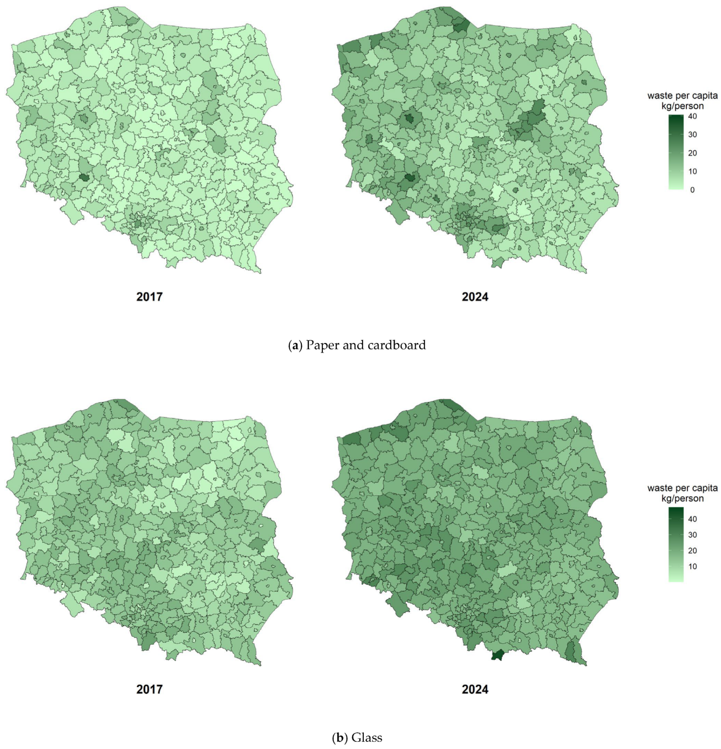
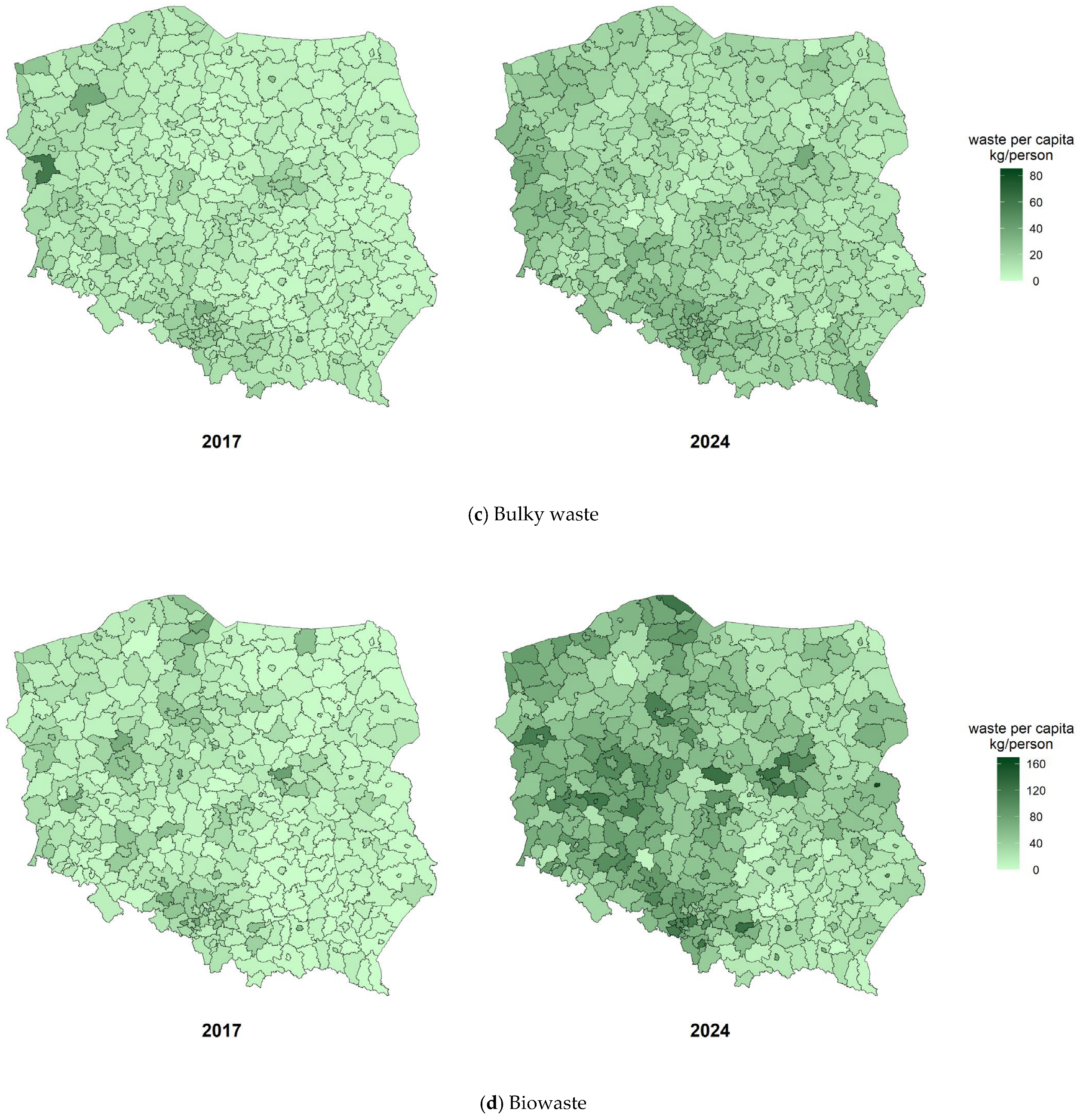
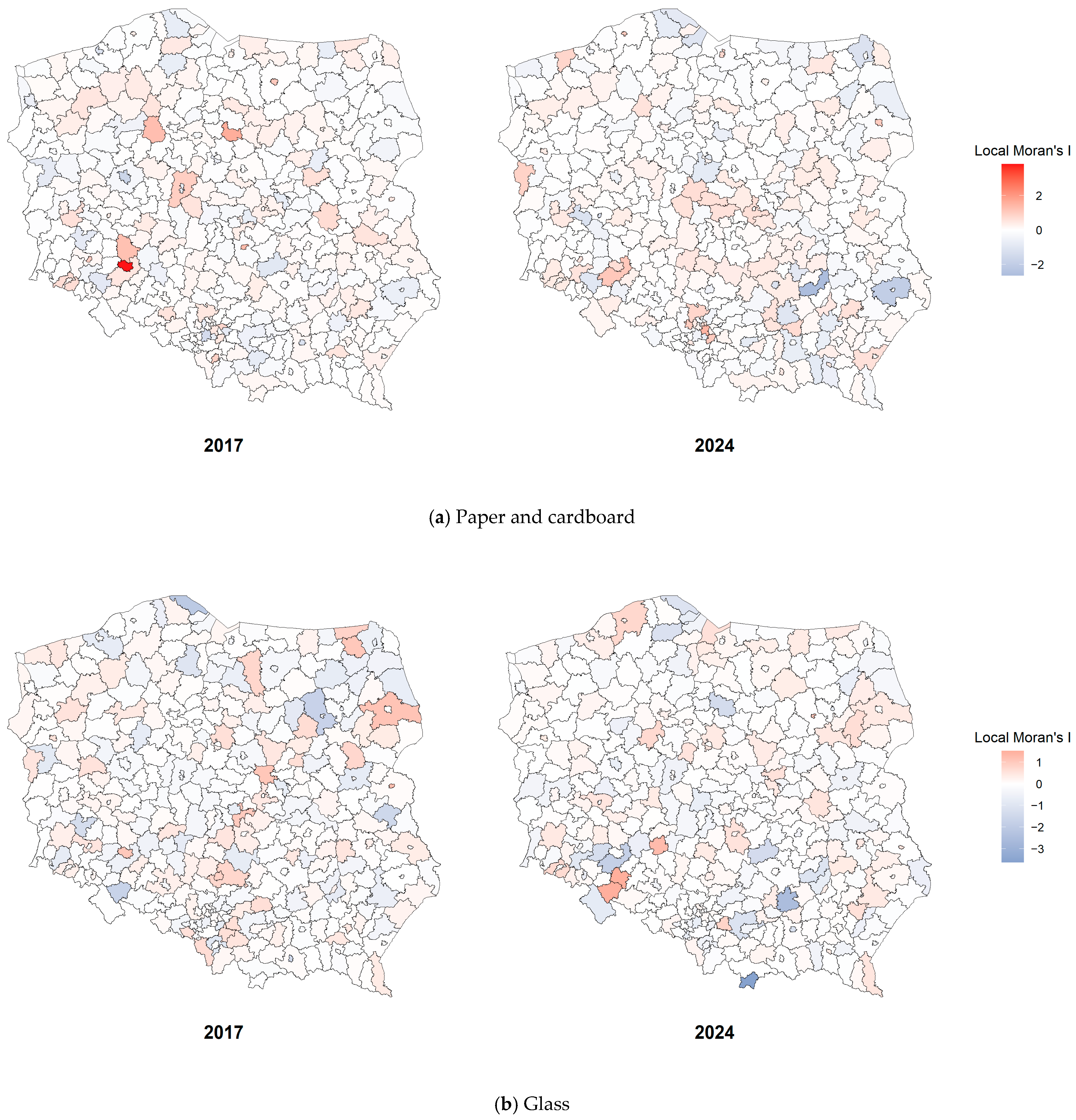
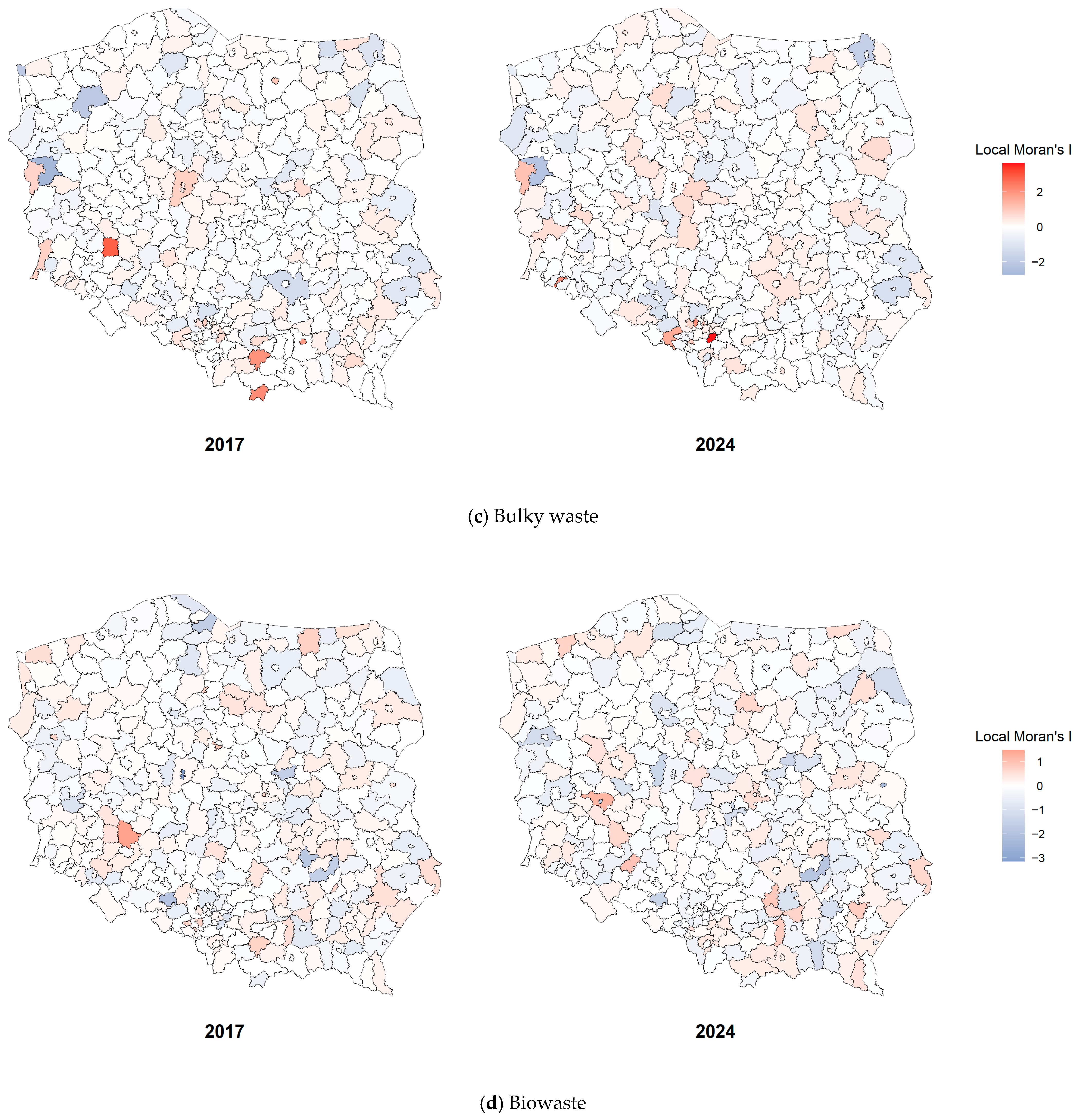
Figure 2 and Figure 3 present the spatial distributions of waste fractions—paper and cardboard, glass, bulky waste, and biowaste—as well as the corresponding local Moran’s I statistics. The inclusion of local Moran’s I serves as a preliminary diagnostic tool to assess the presence of spatial effects, which may warrant incorporation into the subsequent econometric models.
Figure 2a illustrates a general increase over time in the recorded quantities of household paper and cardboard waste. The 2024 pattern shows higher per capita levels across most regions compared with 2017, with notably elevated values in selected northern and southern areas. Despite the overall rise, regional variation persists. A similar trend can be observed with regard to other waste fractions (Figure 2b–d).
Taking into account Local Moran’s I statistics for household paper and cardboard waste in 2017 (Figure 3a), only a few municipalities show statistically notable positive clusters, indicated by localised concentrations of high values surrounded by similarly high levels, as well as occasional negative clusters where low values are adjacent to higher ones. By 2024, the pattern becomes more dispersed, with fewer distinct areas exhibiting strong local autocorrelation. The reduced intensity and spatial concentration of both positive and negative clusters suggest a weakening of localised clustering over time, implying a more spatially diffuse distribution of paper waste generation. For glass waste (Figure 3b), the Local Moran’s I results reveal a similarly limited degree of spatial clustering. In 2017, isolated positive and negative clusters appeared, indicating localised groupings of relatively high or low per capita values, but these patterns are neither extensive nor strongly concentrated. By 2024, the spatial structure remains weak, with a scattered distribution of both high-high and low-low associations and no persistent regional concentrations.

4.2. Spatial Panel Models of Waste Fractions

The Kuznets effect is examined using a spatial panel data framework. Equation (1) is estimated for each waste fraction, both without and with spatial effects. The choice between fixed-effects (FE) and random-effects (RE) specifications was guided by the Hausman test. In all cases, the null hypothesis was rejected in favour of the alternative, leading to the selection of the FE model. To ensure the robustness of the analysis, we also estimated a modified FE specification following Mundlak’s approach [60]. All waste fraction variables (PC, GL, BW, BI), earnings (ER), and tourists per 1000 inhabitants (TR) were log-transformed, allowing the coefficients to reflect proportional changes and capture relative variability across observations.
Furthermore, we considered spatial weight matrices based on contiguity (first- and second-order neighbour structures) and inverse-distance measures. Significant spatial dependencies were identified for the contiguity matrix, and thus, results based on this specification are reported.
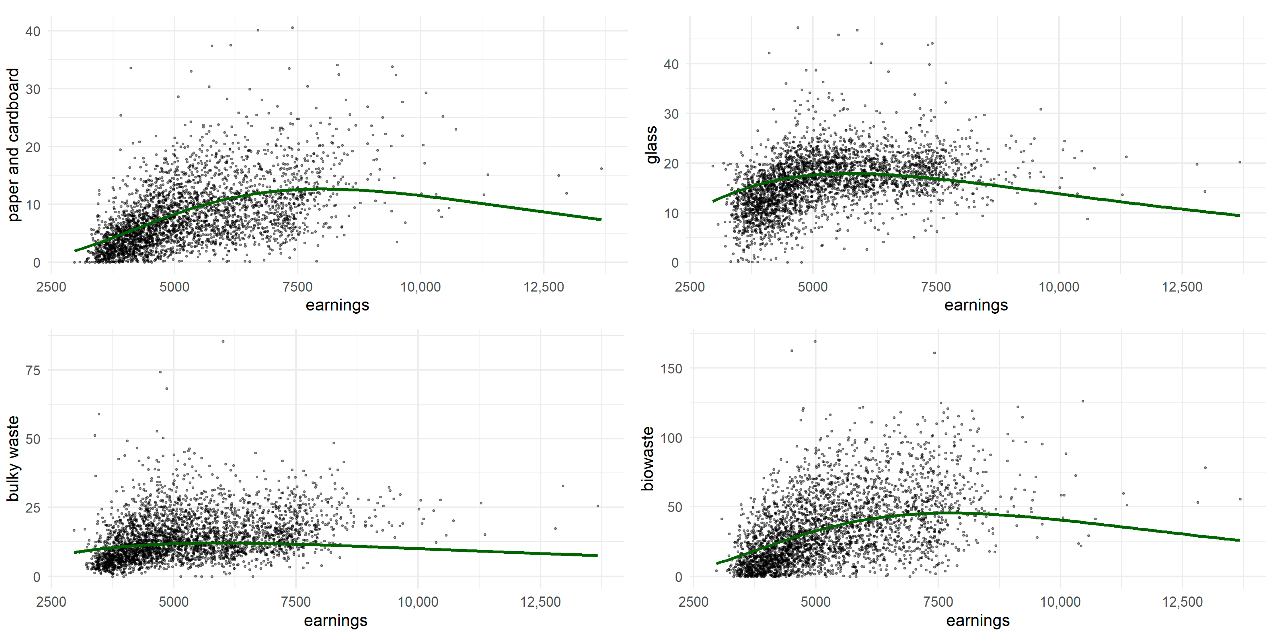
Figure 4 presents the relationship between earnings and per capita municipal waste generation for four waste fractions. Each panel displays observed data points and a fitted curve that reveals a clear inverted U-shaped pattern consistent with the WKC hypothesis. At lower income levels, higher earnings are associated with greater waste generation, whereas beyond a certain threshold, additional income growth is associated with a decline in waste per capita. This turning point is evident across all four fractions. Moreover, the fitted curves closely correspond to the econometric results presented later, supporting the robustness of the WKC interpretation for these waste streams.
Table 3 presents the parameter estimates for the paper and cardboard fraction. Both FE and RE models, using Mundlak’s approach, are presented, including versions with (models 3 and 4) and without (models 1 and 2) spatial effects.
The estimates for paper and cardboard indicate an inverted-U relationship between earnings and paper and cardboard waste in the non-spatial models (Table 3 and Figure 4). The estimated coefficients on ln_ER (>30, p < 0.001) and (ln_ER)2 (<−1.8, p < 0.001) are both statistically significant, yielding turning points of approximately 2020 USD (1870 EUR), which supports the Kuznets effect. In the context of average monthly gross wages in Poland that increased steadily from about 1285 USD (1061 EUR) in 2017 to over 1815 USD (1732 EUR) in 2024, it implies that during the early part of the sample period, many counties were located on the upward-sloping segment of the Waste Kuznets Curve. However, by the later years of the sample, a growing number of counties have reached or exceeded the estimated turning points. These results are consistent with earlier regional WKC studies, which show that turning points are often reached only by a subset of regions and tend to occur at relatively high income levels [11,15]. It also aligns with evidence from EU-wide analyses indicating that waste decoupling is typically partial, gradual, and uneven across space. From a broader perspective, these findings indicate that Poland, as a whole, may be approaching—but has not uniformly surpassed—the income levels at which waste generation stabilises or declines. The coexistence of counties above and below the estimated turning points implies that the national waste system remains structurally heterogeneous. Control variables show that a higher share of older residents (RT > 0, p < 0.01) is associated with more waste, tourism intensity has a small negative influence (ln_TR < 0, p < 0.001), while urbanisation is insignificant. After accounting for spatial dependence (models 3–4), coefficients on ln_ER (≈6.27) and (ln_ER)2 (≈−0.31) become much smaller and statistically weak in FE, indicating that the Kuznets pattern is largely absorbed by spatial spillovers. RT and UR are significant, while tourism becomes statistically insignificant.
The spatial models using the contiguity matrix (Wc) show that paper-cardboard waste is strongly shaped by both local conditions and spillover effects. Earnings have a weak and mixed influence: the spatial coefficient on ln_ER is negative and marginally significant in the FE model (−1.04 *) and close to zero in the RE(M) version, while the impact decomposition indicates small positive direct effects (0.87 *, 0.65 *) and indirect effects of opposite sign (−1.31; 0.97 *). As a result, local income levels are not a dominant driver once spatial interactions are taken into account. By contrast, the share of retirement-age population (RT) shows a consistent and positive association at the spatial level (0.27 ***; 0.09 ***), with large positive indirect impacts and positive total effects, indicating that older demographic structure is linked to higher waste generation and that this tendency propagates to neighbouring areas. Tourism (ln_TR) remains negative, though mostly weak (−0.05), while urbanisation (UR) has a very small effect of a negative sign (−0.01). The spatial lag of waste (ln_PC) is strongly positive (≈0.72–0.73 ***), and the spatial error lag is negative (≈−0.44 ***), showing that counties are influenced by neighbouring waste levels, while past levels dampen current outcomes.
For the glass fraction (Table 4), the spatial coefficients on UR in the Wc component remain close to zero in both specifications (0.021 in FE and 0.003 *** in RE(M)), and the impact decomposition confirms that the magnitude of this relationship is weak. Direct effects are modest, reaching only about 0.023–0.024 *, while indirect effects, although numerically larger (0.115 * and 0.090 ***), still point to a relatively limited role of urbanisation. In contrast, the share of the retirement-age population (RT) shows a more substantial and spatially persistent association with waste generation. The spatial coefficients indicate positive effects in both models (0.127 *** in FE and 0.019 in RE). Direct effects, although modest (0.018 and 0.047 ***), are accompanied by large and strongly positive indirect effects (0.426 *** and 0.233 ***). Tourism retains a negative sign in the spatial coefficients (−0.039 * and −0.026), while the decomposition shows small negative direct effects (−0.014 * and −0.015 *) and moderate negative indirect effects (−0.150 ** and −0.157 **). Spatial indirect effects (−1.363 *** and –0.541) indicate that higher incomes in neighbouring regions are associated with lower waste levels in the region.
Estimates for bulky waste indicate (Table 5) a clear inverse relationship between income and waste generation in non-spatial models. Both ln_ER (≈11.8–12.0, p < 0.001) and its square (≈−0.68, p < 0.001) are highly significant, forming turning points close to 5975 PLN (1387 EUR), p < 0.001) and its square (≈−0.68, p < 0.001) are highly significant, confirming the Kuznets pattern for bulky waste. Among the control variables, the share of residents of retirement age shows a consistent positive effect (RT ≈ 0.13, p < 0.001). Tourism intensity has a slight negative effect (TR ≈ −0.032, p < 0.001), while urbanisation shows a moderate positive effect (UR ≈ 0.029, p < 0.001). When spatial dependence is taken into account, the relationship between income and waste generation becomes significantly weaker. In the spatial FE and RE(M) models, the ln_ER coefficients drop sharply to around 1.0–1.1. The spatial models reveal that bulky waste is shaped by local conditions. The spatial coefficient is negative in the FE model (−0.31) and negative but significant in the RE(M) version (−0.20 ***), suggesting that higher income in neighbouring areas is associated with lower bulky waste locally. Direct effects are small (0.22 and 0.07), while indirect effects are clearly negative (about −0.66 and −0.72 *). As a result, income does not emerge as a dominant driver of bulky waste once the spatial dimension is accounted for. In contrast, the share of the retirement-age population remains a strong and spatially persistent determinant. Direct effects are modest (≈0.05), but indirect effects are large and positive, ranging from 0.21 to 0.25. Tourism continues to show a weak and negative effect, with a very small direct impact and moderate negative spillovers (around −0.13 to −0.15). Urbanisation remains a relatively important determinant in the spatial setting. Direct impacts range from about 0.026 to 0.030, while indirect impacts lie between 0.12 and 0.20.
The parameter estimates from both the non-spatial and spatial models for biowaste (Table 6) exhibit a clear bell-shaped relationship. The coefficients on ln_ER (31.1–31.3 ***) and (ln_ER)2 (−1.7 ***) are both highly statistically significant, implying a turning point at an earnings level of 7753 PLN (1800 EUR). Beyond this threshold, per capita biowaste generation begins to decline. This turning point corresponds closely to the average wage levels observed in Poland (1732 EUR). This suggests that a substantial share of Polish counties may have reached or slightly surpassed the income threshold at which the scale effect of income on waste generation weakens and technique and composition effects begin to dominate. Among the control variables, the share of residents of retirement age and tourism intensity are highly statistically significant in the non-spatial models. The former (RT = 0.15 ***) has a positive effect on biowaste generation, whereas the latter (ln_TR = −0.15 ***) has a clearly negative impact. The effect of urbanisation is slightly positive but statistically insignificant.
Incorporating spatial effects into the analysis provides additional insights into these relationships. The overall positive effect of residents of retirement age is found to be driven primarily by spillover effects from neighbouring regions, with an estimated indirect impact of 0.20 to 0.28. A similar pattern emerges for tourism, with an estimated indirect effect of approximately −0.17. In contrast to the non-spatial models, the effect of urbanisation changes substantially once spatial dependence is accounted for, revealing a statistically significant positive impact that arises both within the county and from neighbouring counties.

5. Discussion

For paper and cardboard waste, non-spatial specifications suggest an inverted-U relationship with income; however, this pattern weakens substantially once spatial dependence is introduced. In the fixed-effects spatial model, income coefficients decline sharply in both magnitude and statistical significance, indicating that the apparent Kuznets effect is partly driven by spatial spillovers rather than purely local economic conditions. A similar pattern is observed for glass waste, where income effects are generally weak and mixed. Direct effects are small and often insignificant, while negative indirect effects suggest that higher income levels in neighbouring regions are associated with lower local glass waste generation. In contrast, bulky waste exhibits a clearer Kuznets-type relationship with income. Although an inverted-U pattern is evident in non-spatial models, once spatial interactions are modelled explicitly, the income coefficients shrink in magnitude and lose significance, and the indirect impacts become negative.
Demographic structure emerges as one of the most stable and influential determinants of waste generation across all fractions, although its impact is not uniform across waste categories. For paper and cardboard waste, a higher share of elderly residents within a region exerts a significant negative effect, which may indicate lower environmental awareness among older individuals or reflect differences in consumption patterns. This finding is consistent with earlier observations by Struk and Soukopová [54], who report that people aged 50–79 tend to generate relatively high amounts of residual waste per capita while sorting the least. For glass waste, both direct and indirect effects suggest that age structure consistently explains variations in glass waste volumes. In the case of bulky waste, population ageing plays an even more pronounced role. Regions with a higher proportion of elderly residents generate more bulky waste locally, and this effect extends to neighbouring regions, indicating the presence of spatial spillovers. At first glance, these results appear to contradict those of the OECD [61], which suggest that age is associated with lower household waste generation, as well as the findings of Rybova [55], where this relationship is reported to be insignificant, and Liu et al. [51], who associate a higher demographic dependency ratio with lower municipal waste generation due to reduced income levels and consumption intensity. However, these studies rely predominantly on aggregated measures of total waste, whereas our fraction-level analysis reveals a heterogeneous influence of demographic structure. As population ageing increases the generation of certain waste fractions while reducing others, opposing effects may offset each other in aggregate indicators. Our results, therefore, point to an accumulation and tidying effect: older individuals are more likely to organise their households and dispose of accumulated goods over a long life. It should be noted, however, that the observed “tidying effect” may not reflect a permanent age-related behavioural pattern but rather a transitory cohort effect, similar to Florczak and Jabłonowski’s [62] observations. The current elderly population in Poland belongs to cohorts that accumulated durable goods over long periods under conditions of scarcity and lower replacement rates, which may lead to higher disposal of bulky items at later stages of life. As younger cohorts are characterised by different consumption patterns and shorter product lifecycles, this effect may weaken or change in nature.
Urbanisation plays only a limited role in explaining waste generation once spatial interactions are taken into account. For paper and cardboard waste, urbanisation is statistically significant in some specifications but remains very weak in magnitude, indicating that settlement structure does not substantially affect waste generation. It is in line with Lu et al. [57] that municipal solid waste scales linearly with urban population, and urbanisation itself (city size) does not show a significant accelerated increase in waste. For glass waste, urbanisation increases waste levels, but its effect is marginal. The fact that the spatial coefficients of UR remain close to zero further confirms that urbanisation does not significantly change waste levels. In contrast, bulky waste shows a more noticeable response to urbanisation. Urban areas tend to generate higher volumes of bulky waste. The observed positive association between urban areas and bulky waste generation aligns with Chen’s [56] definition of urbanisation, which integrates demographic concentration, infrastructure development, industrial activity, and income growth—factors that jointly intensify consumption and replacement of durable household goods.
The impact of tourism on waste generation is consistently weak and negative across all waste fractions. For paper and cardboard waste, tourism inflows do not substantially increase waste generation, suggesting that tourism-related waste is either limited or effectively managed through seasonal waste management practices. A similar pattern is observed for glass waste. For bulky waste, tourism effects remain weak and negative, suggesting that bulky waste associated with tourism activities is minimal. Overall, our results are consistent with those of Diaz-Farina et al. [58] and Arbulu et al. [59], who pointed out that although tourism contributes to the generation of mixed waste, the direct impact of tourists on waste amounts is relatively small compared to that of residents.

6. Conclusions

The aim of this study was to examine the relationship between income and municipal waste generation within the Waste Kuznets Curve framework, with a focus on disaggregated household waste fractions. In particular, using county-level panel data, we examined whether non-linear income–waste relationships persist after accounting for spatial dependence.
Our results extend previous research in several important ways. First, while most empirical WKC studies focus on aggregated municipal solid waste at national or regional levels, this study analyses disaggregated household waste fractions—paper and cardboard, glass, bulky waste, and biowaste. Earlier contributions examining disaggregated waste streams have largely concentrated on specific categories such as e-waste, medical waste, or construction waste (e.g., Boubellouta and Kusch-Brandt [25]; Wang et al. [23]), often at highly aggregated spatial scales. By contrast, the present study captures fraction-specific income responses within a unified WKC framework. Second, the study advances earlier spatial analyses of the WKC. While regional or country-level studies exist (e.g., Ercolano et al. [11]; Madden et al. [14]), they typically treat spatial interactions only implicitly or descriptively. By employing county-level panel data, this study provides a finer spatial perspective that enables the explicit identification of both local effects and spillovers, thereby extending earlier work, such as Gui et al. [13]. Third, from a methodological perspective, our results show that inverted-U income–waste relationships weaken when spatial dependence is taken into account. This finding contributes to recent methodological concerns of WKC estimation (e.g., Schneider [40]) by demonstrating that conclusions about income-driven waste decoupling may be biased upward when regions are treated as independent units.
Considering practical recommendations, our research suggests that waste management policy should not be based solely on assumptions about waste reduction linked to economic growth. Our research indicates that inter-municipal cooperation and coordinated regional strategies may be more effective than isolated local interventions. In practical terms, such coordination may take several complementary forms. For example, municipalities can jointly develop and operate shared waste-sorting and treatment facilities, enabling economies of scale and reducing infrastructure duplication. Coordinated information and education campaigns, implemented at the regional level, can ensure consistent messaging on waste separation, thereby reinforcing behavioural change beyond administrative boundaries. Other forms of inter-municipal cooperation may include joint procurement of waste services and coordinated planning of waste-management investments. Secondly, the strong influence of demographic structure suggests that population ageing should be taken into account in the design of waste policy. Tailored information campaigns, simplified sorting systems, and collection services adapted to the needs of older people can improve waste sorting. Thirdly, tourism-related waste should not be overstated in local waste policy. Policy efforts should focus on resident-driven waste generation while allowing for flexible seasonal adjustments in tourist destinations as necessary.
The study is subject to several limitations. As income is proxied by average earnings, it may not fully capture household purchasing power or income heterogeneity within regions. Future studies could address this limitation by using alternative measures such as disposable or median household income or consumption-based indicators. Moreover, while the empirical results are context-specific to Poland, the econometric framework is general and can be applied to regions in other countries, potentially augmented with additional control variables reflecting institutional or socio-economic differences. Consequently, the findings may not be directly generalisable to countries with different waste management policies or consumption patterns. Importantly, during the period 2017–2024, Poland did not implement a single, clearly defined structural reform of its waste-management regulatory framework; rather, changes were incremental and focused mainly on fee adjustments and the expansion of selective collection obligations. Such institutional adjustments may reduce waste generation through mandatory sorting rules. As a result, the observed decline in waste may appear to be a technique effect within the Waste Kuznets Curve framework, even though it is driven by regulation rather than income-induced technological change. Future research should extend the analysis to a cross-country setting to assess the robustness of the findings. Applying the same spatial and disaggregated approach to other countries would enable comparative analysis and allow conclusions to be drawn regarding the homogeneity or heterogeneity of the estimated effects across institutional contexts.

Author Contributions

Conceptualisation, methodology, software, validation, formal analysis, investigation, resources, data curation, writing—original draft preparation, writing—review and editing, visualisation, supervision, project administration, funding acquisition: A.K. (Arkadiusz Kijek) and A.K. (Agnieszka Karman) All authors have read and agreed to the published version of the manuscript.

Funding

This research received no external funding.

Institutional Review Board Statement

Not applicable.

Informed Consent Statement

Not applicable.

Data Availability Statement

The database is available on Zenodo at https://doi.org/10.5281/zenodo.18184103. The analysis was performed using STATA 19 and R 4.5.1.

Conflicts of Interest

The authors declare no conflicts of interest.

References

  1. Kaza, S.; Yao, L.; Bhada-Tata, P.; Van Woerden, F. What a Waste 2.0: A Global Snapshot of Solid Waste Management to 2050; World Bank: Washington, DC, USA, 2018. [Google Scholar]
  2. Ari, I.; Sentürk, H. The relationship between GDP and methane emissions from solid waste: A panel data analysis for the G7. Sustain. Prod. Consum. 2020, 23, 282–290. [Google Scholar] [CrossRef]
  3. Arbulú, L.J.; Rey-Maquieira, J. Tourism and solid waste generation in Europe: A panel data assessment of the environmental Kuznets curve. Waste Manag. 2015, 46, 628–636. [Google Scholar] [CrossRef]
  4. Pan, A.; Yu, L.; Yang, Q. Characteristics and Forecasting of Municipal Solid Waste Generation in China. Sustainability 2019, 11, 1433. [Google Scholar] [CrossRef]
  5. İçen, H.; Çil, N. Investigating municipal waste Kuznets curve for 22 OECD countries. Environ. Monit. Assess. 2023, 195, 1506. [Google Scholar] [CrossRef]
  6. Voukkali, I.; Papamichael, I.; Loizia, P.; Zorpas, A.A. Urbanization and solid waste production: Prospects and challenges. Environ. Sci. Pollut. Res. 2024, 31, 17678–17689. [Google Scholar] [CrossRef]
  7. Lee, S.; Kim, J.; Chong, W.K. Causes of municipal solid waste and greenhouse gas emissions from the waste sector in the United States. Waste Manag. 2016, 56, 593–599. [Google Scholar] [CrossRef]
  8. Magazzino, C.; Mele, M.; Schneider, N. The relationship between municipal solid waste and greenhouse gas emissions: Evidence from Switzerland. Waste Manag. 2020, 113, 508–520. [Google Scholar] [CrossRef]
  9. Gui, X.D.; Li, H.M. Empirical study of environmental Kuznets curve. China Popul. Resour. Environ. 2010, 5, 5–8. [Google Scholar]
  10. Farhani, S.; Mrizak, S.; Chaibi, A.; Rault, C. The environmental Kuznets curve and sustainability: A panel data analysis. Energy Policy 2014, 71, 189–198. [Google Scholar] [CrossRef]
  11. Ercolano, S.; Gaeta, L.; Ghinoi, S.; Silvestri, F. Kuznets curve in municipal solid waste production: An empirical analysis based on municipal-level panel data from Lombardy (Italy). Ecol. Indic. 2018, 93, 397–403. [Google Scholar] [CrossRef]
  12. Trujillo-Lora, J.C.; Carrillo, B.B.; Charris Vizcaíno, C.A.; Iglesias-Pinedo, W.J. The environmental Kuznets curve (EKC): An analysis of landfilled solid waste in Colombia. Rev. Fac. Cienc. Econ. 2013, 21, 7–16. [Google Scholar]
  13. Gui, S.; Zhao, L.; Zhang, Z. Does municipal solid waste generation in China support the environmental Kuznets curve? New evidence from spatial linkage analysis. Waste Manag. 2019, 84, 310–319. [Google Scholar] [CrossRef]
  14. Madden, B.J.; Florin, N.; Mohr, S.; Giurco, D. Using the waste Kuznets curve to explore regional variation in the decoupling of waste generation and socioeconomic indicators. Resour. Conserv. Recycl. 2019, 149, 674–686. [Google Scholar] [CrossRef]
  15. Gnonlonfin, A.; Kocoglu, Y.; Péridy, N. Municipal solid waste and development: Environmental Kuznets curve evidence for Mediterranean countries. Reg. Dev. 2017, 45, 113–130. [Google Scholar]
  16. Ichinose, D.; Yamamoto, M.; Yoshida, Y. Reexamining the Waste–Income Relationship; GRIPS Discuss. Pap., 10-31; National Graduate Institute for Policy Studies: Tokyo, Japan, 2011; pp. 10–31. [Google Scholar]
  17. Jaligot, R.; Chenal, J. Decoupling municipal solid waste generation and economic growth in the canton of Vaud, Switzerland. Resour. Conserv. Recycl. 2018, 130, 260–266. [Google Scholar] [CrossRef]
  18. Chen, C. Spatial inequality in municipal solid waste disposal across regions in developing countries. Int. J. Environ. Sci. Technol. 2010, 7, 447–456. [Google Scholar] [CrossRef]
  19. Wang, H.; Nie, Y. Municipal solid waste characteristics and management in China. J. Air Waste Manag. Assoc. 2001, 51, 250–263. [Google Scholar] [CrossRef]
  20. Su, E.C.Y.; Chen, Y.T. Policy or income to affect the generation of medical wastes: An application of the environmental Kuznets curve using Taiwan as an example. J. Clean. Prod. 2018, 188, 489–496. [Google Scholar] [CrossRef]
  21. Rom, P.; Guillotreau, P. Mismanaged plastic waste and the environmental Kuznets curve: A quantile regression analysis. Mar. Pollut. Bull. 2024, 202, 116320. [Google Scholar] [CrossRef]
  22. Mann, S.; Bobeică, M.; Beciu, S.; Arghiroiu, G.A. Is there a food waste Kuznets curve? Evidence from China, Romania, and Switzerland. Environ. Prot. Res. 2023, 3, 233–245. [Google Scholar] [CrossRef]
  23. Wang, B.; Jia, R.; Xu, J.; Wei, Y.; Li, Q.; Yao, Y.; Zhu, X.; Xu, A.; Zhang, J. Research on environmental Kuznets curve of construction waste generation based on China’s provincial data. Sustainability 2024, 16, 5610. [Google Scholar] [CrossRef]
  24. Xu, X.; Zhang, X.; Wu, Q. Testing the existence of the waste Kuznets curve hypothesis in 45 emerging economies: Evidence from an e-waste panel data survey. J. Environ. Manag. 2025, 373, 123812. [Google Scholar]
  25. Boubellouta, B.; Kusch-Brandt, S. Determinants of e-waste composition in the EU28+2 countries: A panel quantile regression evidence of the STIRPAT model. Int. J. Environ. Sci. Technol. 2022, 19, 10493–10510. [Google Scholar] [CrossRef]
  26. Grossman, G.M.; Krueger, A.B. Environmental Impacts of a North American Free Trade Agreement; NBER Work. Pap.; NBER: Cambridge, MA, USA, 1991; 3914p. [Google Scholar]
  27. Shafik, N.; Bandyopadhyay, S. Economic Growth and Environmental Quality: Time Series and Cross-Country Evidence; World Dev. Rep. 1992 Background Pap; The World Bank: Washington, DC, USA, 1992. [Google Scholar]
  28. Holtz-Eakin, D.; Selden, T.M. Stoking the Fires? CO2 Emissions and Economic Growth; NBER Work. Pap.; NBER: Cambridge, MA, USA, 1992; 4248p. [Google Scholar]
  29. Chavas, J.P. On impatience, economic growth and the EKC: A dynamic analysis of resource management. Environ. Resour. Econ. 2004, 28, 123–152. [Google Scholar]
  30. Andreoni, J.; Levinson, A. The simple analytics of the environmental Kuznets curve. J. Public Econ. 2001, 80, 269–286. [Google Scholar] [CrossRef]
  31. Brock, W.A.; Taylor, S.M. The Green Solow Model; NBER Work. Pap.; NBER: Cambridge, MA, USA, 2004; p. 10557. [Google Scholar]
  32. Sinha, A.; Schneider, N.; Song, M.; Shahzad, U. The determinants of solid waste generation in the OECD: Evidence from cross-elasticity changes in a common correlated effects framework. Resour. Conserv. Recycl. 2022, 182, 106322. [Google Scholar] [CrossRef]
  33. Mazzanti, M.; Zoboli, R. Municipal waste Kuznets curves: Evidence on socio-economic drivers and policy effectiveness from the EU. Environ. Resour. Econ. 2009, 44, 203–230. [Google Scholar] [CrossRef]
  34. Mele, M.; Magazzino, C.; Schneider, N.; Gurrieri, A.R.; Golpira, H. Innovation, income, and waste disposal operations in Korea: Evidence from spectral Granger causality and artificial neural networks. Econ. Polit. 2022, 39, 1–33. [Google Scholar]
  35. Halpern, A.L. The Economics of Sustainable Development; Cambridge University Press: Cambridge, UK, 1995. [Google Scholar]
  36. Sjostrom, M.; Ostblom, G. Decoupling waste generation from economic growth—A CGE analysis of the Swedish case. Ecol. Econ. 2010, 69, 1545–1552. [Google Scholar] [CrossRef]
  37. Coase, R.H. The problem of social cost. J. Law Econ. 1960, 3, 1–44. [Google Scholar] [CrossRef]
  38. Mazzanti, M. Is waste generation de-linking from economic growth? Empirical evidence for Europe. Appl. Econ. Lett. 2008, 15, 287–291. [Google Scholar] [CrossRef]
  39. Liddle, B. Population, affluence, and environmental impact across development: Evidence from panel cointegration modeling. Environ. Model. Softw. 2013, 40, 255–266. [Google Scholar] [CrossRef]
  40. Schneider, N. Endogeneity and other problems in curvilinear income–waste response function estimations. Stoch. Environ. Res. Risk Assess. 2024, 38, 357–382. [Google Scholar]
  41. Gardiner, R.; Hájek, P. Municipal waste generation, R&D intensity, and economic growth nexus: A case of EU regions. Waste Manag. 2020, 114, 124–135. [Google Scholar]
  42. Halkos, G.; Petrou, K.N. The relationship between MSW and education: WKC evidence from 25 OECD countries. Waste Manag. 2020, 114, 240–252. [Google Scholar] [CrossRef] [PubMed]
  43. Ma, Y.; Jia, L.X.; Hou, Y.; Wu, X. The impact of economic growth and tiered medical policy on medical waste generation: An empirical analysis based on the environmental Kuznets curve model. Front. Environ. Sci. 2022, 10, 873921. [Google Scholar] [CrossRef]
  44. Konat, G.; Dürrü, Z.; Han, A. Investigation of waste Kuznets curve hypothesis in selected OECD member EU countries: Panel data analysis. Akad. Yaklaşımlar Derg. 2024, 15, 1028–1049. [Google Scholar]
  45. Cavalheiro, E.A.; Machado, R.H.; Castro, A.S.; Falck, L.R. Urban solid waste generation and GDP per capita: A global analysis through the lens of the environmental Kuznets curve. Contrib. Cienc. Soc. 2024, 17, e5574. [Google Scholar]
  46. Soukiazis, E.; Proença, S. Exploring the driving forces of waste generation in Portuguese municipalities. Environ. Dev. Econ. 2020, 26, 340–363. [Google Scholar] [CrossRef]
  47. Kusch, S.; Hills, C.D. The link between e-waste and GDP: New insights from pan-European data. Resources 2017, 6, 15. [Google Scholar]
  48. Boubellouta, B.; Kusch-Brandt, S. Relationship between economic growth and mis-managed e-waste: Panel data evidence from 27 EU countries analyzed under the Kuznets curve hypothesis. Waste Manag. 2021, 120, 85–97. [Google Scholar]
  49. Shahbaz, M.; Sinha, A. Environmental Kuznets curve for CO2 emissions: A literature survey. J. Econ. Stud. 2019, 46, 106–130. [Google Scholar] [CrossRef]
  50. Dinda, S. Environmental Kuznets curve hypothesis: A survey. Ecol. Econ. 2004, 49, 431–455. [Google Scholar] [CrossRef]
  51. Liu, X.; Wang, W.; Lu, S.; Wang, Y.F.; Ren, Z. Analysis of the relationship between economic growth and industrial pollution in Zaozhuang, China—Based on the hypothesis of the environmental Kuznets curve. Environ. Sci. Pollut. Res. 2016, 23, 16349–16358. [Google Scholar] [CrossRef]
  52. Campos, J.; Ericsson, N.R.; Hendry, D.F. General-to-specific modeling: An overview and selected bibliography. Int. Finance Discuss. Pap. 2005, 10, 838. [Google Scholar]
  53. Mazzanti, M.; Zoboli, R. Delinking and environmental Kuznets curves for waste indicators in Europe. Environ. Sci. 2005, 2, 409–425. [Google Scholar] [CrossRef]
  54. Struk, M.; Soukopová, J. Age structure and municipal waste generation and recycling—New challenge for the circular economy. In Proceedings of the Cyprus International Conference on Sustainable Solid Waste Management, Nicosia, Cyprus, 23–25 June 2016. [Google Scholar]
  55. Rybova, K. Do sociodemographic characteristics in waste management matter? Case study of recyclable generation in the Czech Republic. Sustainability 2019, 11, 2030. [Google Scholar] [CrossRef]
  56. Chen, Y.-C. Effects of urbanization on municipal solid waste composition. Waste Manag. 2018, 79, 828–836. [Google Scholar] [CrossRef]
  57. Lu, M.; Zhou, C.; Wang, C.; Jackson, R.B.; Kempes, C.P. Worldwide scaling of waste generation in urban systems. Nat. Cities 2024, 1, 126–135. [Google Scholar] [CrossRef]
  58. Díaz-Fariña, E.; Díaz-Hernández, J.J.; Padrón-Fumero, N. The contribution of tourism to municipal solid waste generation: A mixed demand–supply approach on the island of Tenerife. Waste Manag. 2020, 102, 587–597. [Google Scholar]
  59. Arbulú, I.; Rey-Maquieira, J.; Sastre, F. The impact of tourism and seasonality on different types of municipal solid waste (MSW) generation: The case of Ibiza. Heliyon 2024, 10, e5574. [Google Scholar] [CrossRef] [PubMed]
  60. Mundlak, Y. On the pooling of time series and cross-sectional data. Econometrica 1978, 56, 69–86. [Google Scholar] [CrossRef]
  61. OECD. Household Waste Practices: New Empirical Evidence and Policy Implications for Sustainable Behaviour; OECD Environment Working Papers, No. 249; OECD Publishing: Paris, France, 2024; Available online: https://www.oecd.org/en/publications/household-waste-practices_9e5e512c-en.html (accessed on 20 December 2025).
  62. Florczak, A.; Jabłonowski, J. Consumption over the Life Cycle in Poland; NBP Work. Pap.; Narodowy Bank Polski: Warsaw, Poland, 2016; No. 252. [Google Scholar]
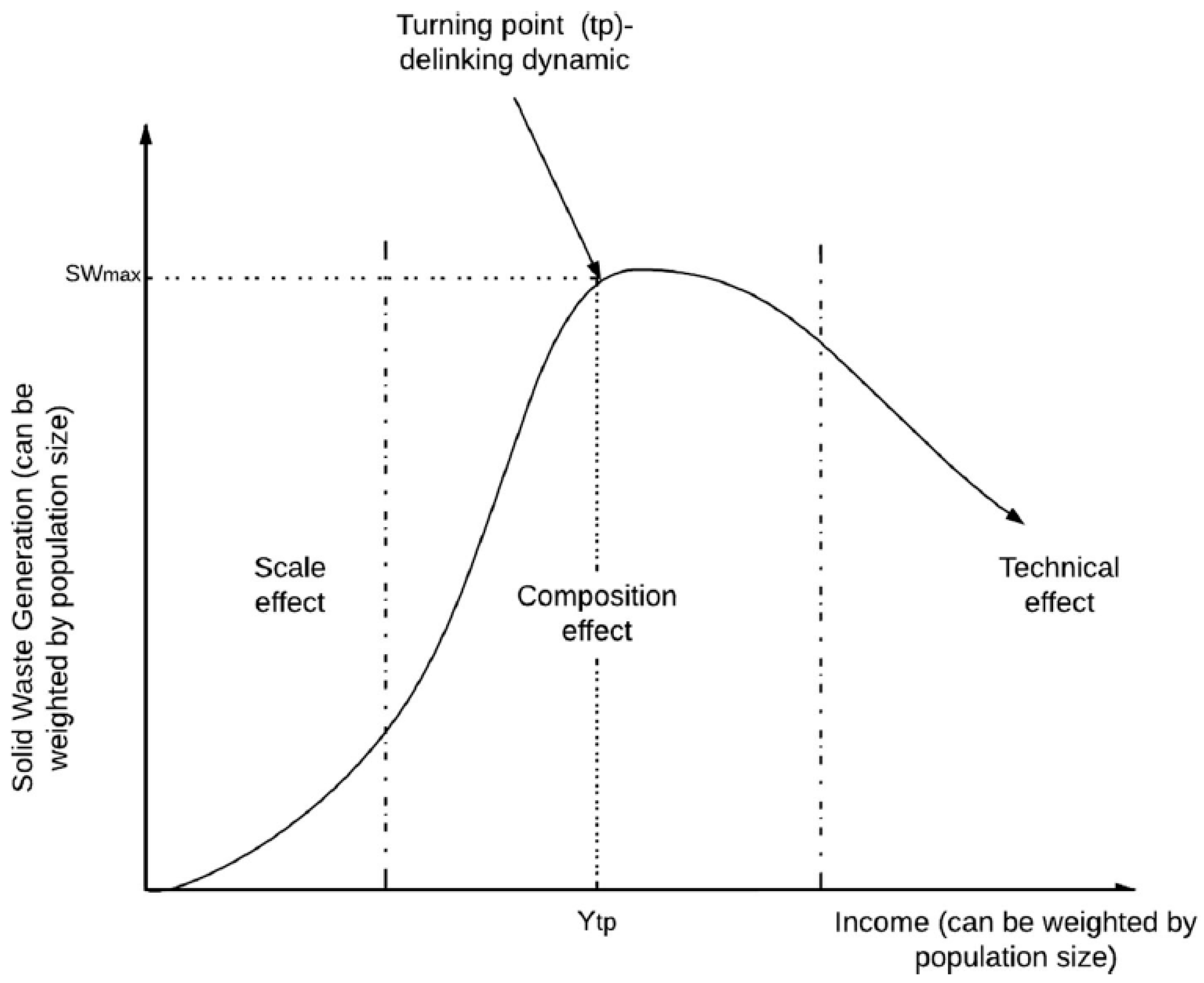
Figure 1. Stylised representation of the Waste Kuznets Curve [40].
Sustainability 18 01204 g001
Figure 2. Household waste per capita in Polish counties in 2017 and 2024.
Sustainability 18 01204 g002aSustainability 18 01204 g002b
Figure 3. Local Moran’s I of household waste in Polish counties in 2017 and 2024.
Sustainability 18 01204 g003aSustainability 18 01204 g003b
Figure 4. Waste Kuznets Curve—waste fraction vs. earnings.
Sustainability 18 01204 g004
Table 1. Selected empirical studies on the Waste Kuznets Curve.
Authors
(Year)
Regional UnitsWaste CategoryConclusionsAnalysis Methods
Gnonlonfin et al. (2017) [15]Mediterranean countriesMunicipal solid wasteEKC holds mainly for developed countries with very high turning points; for most Mediterranean countries, EKC does not imply short-term MSW reduction Panel data with controls and missing-data imputation
Ercolano et al. (2018) [11]Lombardy, ItalyMunicipal solid wastePartial WKC support; few municipalities reached a turning point, and many had not yet decoupledMunicipal-level panel regressions
Jaligot, Chenal (2018) [17]The canton of Vaud, SwitzerlandMunicipal wasteTax point value (income) (+), tax point value (income2) (−)Panel regressions
Gui et al. (2019) [13]Chinese citiesMunicipal solid wasteNo inverted-U; spatial linkage analysis showed MSW did not follow EKC and instead indicated an ongoing positive association with income in many cities Spatial linkage analysis
Madden et al. (2019) [14]New South Wales, AustraliaMunicipal wasteMany rural municipalities conformed to WKC; tipping-point ratios varied regionally, indicating relative decoupling in places Geographically and temporally weighted regression (GTWR)
Ari, Sentürk (2020) [2]G7 countriesCH4
Emissions
Cubic model: GDP (−),
GDP2 (+), GDP3 (−), urbanisation (+)
Panel ARDL
Halkos, Petrou (2020) [42]25 OECD countries.Municipal solid wasteAn inverted U-shape relationship is observed. Interdependence between waste, economic growth and education level.Panel unit root tests
Gardiner, Hajek (2020) [41]Old and new EU countriesMunicipal wasteOld EU countries: GDP (+), R&D intensity (+), heating energy (+), employment rate (+), gross fixed capital (+)
New EU countries: GDP (+), R&D intensity (+), heating energy (+), employment rate (−), gross fixed capital (−)
Panel cointegration and
causality
Boubellouta, Kusch-Brandt (2022) [25]EU28+2 countriesDisaggregated e-waste categoriesConfirmed inverted-U across nearly all quantiles and pooled OLS for all categories, indicating EKC for e-waste categories STIRPAT + panel quantile regression and pooled OLS
Ma et al. (2022) [43]Eight Chinese citiesMedical wasteFound N-shaped relation and policy (tiered medical reform) altered waste dynamics EKC models with policy controls and panel data
Rom, Guillotreau (2024) [21]136 field observation data points located in 67 rivers and 14 countriesPlastic wasteThe relationship between economic growth and MPW is not monolithic. In the lower quantiles, up to the 40th percentile, economic growth does not manifest the traditional EKC trajectory. In higher quantiles of plastic waste, the classical EKC relationship begins to take shape.Quantile regression
Mann et al. (2023) [22]1510 Chinese, Romanian and Swiss householdsFood wasteThe concept of EKC can be applied to the problem of food waste. Romanian and Chinese consumers declare more food waste than those in Switzerland, and the differences between the countries can be explained by differences in attitudes and behaviour.Logit model
Konat et al. (2024) [44]Top ten countries with the highest urban solid waste generation among the OECD member EU countriesUrban solid wasteThe negative relationship between per capita urban solid waste generation and per capita real income is invalid. Control variables such as the Human Development Index, population density, and the unemployment rate significantly affect per capita urban solid waste generation.Panel regression model
Wang et al. (2024) [23]31 Chinese provinces, municipalities, and autonomous regionsConstruction wasteThe findings reveal an N-shaped curve pattern for construction waste per capita. The factors influencing construction waste generation are the added value of the secondary industry, labour productivity in the construction industry, GDP per capita, urbanisation rate, year-end resident population, and the technical equipment rate of construction enterprises. Panel data
Xu et al. (2025) [24]45 emerging economiese-wasteThe relationship between economic growth and e-waste imports exhibits an inverted U-shaped curve. Most emerging economies remain in a low-income non-decoupling state, with only a few countries achieving high-income absolute decoupling. Panel data
Gnonlonfin et al. (2017) [15]Mediterranean countriesMunicipal solid wasteEKC holds mainly for developed countries with very high turning points; for most Mediterranean countries, EKC does not imply short-term MSW reduction Panel data with controls and missing-data imputation
Ercolano et al. (2018) [11]Lombardy, ItalyMunicipal solid wastePartial WKC support; few municipalities reached a turning point, and many had not yet decoupled Municipal-level panel regressions
Jaligot, Chenal (2018) [17]The canton of Vaud, SwitzerlandMunicipal wasteTax point value (income) (+), tax point value (income2) (−)Panel regressions
Gui et al. (2019) [13]Chinese citiesMunicipal solid wasteNo inverted-U; spatial linkage analysis showed MSW did not follow EKC and instead indicated an ongoing positive association with income in many cities Spatial linkage analysis
Madden et al. (2019) [14]New South Wales, AustraliaMunicipal wasteMany rural municipalities conformed to WKC; tipping-point ratios varied regionally, indicating relative decoupling in places Geographically and temporally weighted regression (GTWR)
Ari, Sentürk (2020) [2]G7 countriesCH4
Emissions
Cubic model: GDP (−),
GDP2 (+), GDP3 (−), urbanisation (+)
Panel ARDL
Table 2. Average waste fractions per capita (kg/person) by urban and rural counties, 2017 and 2024.
YearCounty TypeWaste Fraction
Paper and CardboardGlassBulky WasteBiowaste
2017Urban6.19.912.727.1
Rural3.411.28.415.5
2024Urban17.216.923.160
Rural9.71916.849.1
Table 3. Estimates of the spatial panel models for household paper and cardboard.
(1) FE(2) RE(M)(3) FE(4) RE(M)
ln_PCln_PCln_PCln_PC
Main
ln_ER33.07 ***34.01 ***6.271 *11.24 ***
(ln_ER)2−1.838 ***−1.892 ***−0.314−0.621 ***
RT0.0742 **0.0712 **−0.133 ***−0.0604 **
ln_TR−0.0495 ***−0.0489 ***−0.0062−0.0115
UR0.02340.02320.0443 ***0.0397 **
cons−149.1 ***−148.9 *** −50.34 ***
Wc
ln_ER −1.038 *−0.197 *
RT 0.267 ***0.0924 ***
ln_TR −0.0524−0.0507 *
UR −0.0198−0.00762 ***
ln_PC 0.716 ***0.733 ***
e.ln_PC −0.442 ***−0.464 ***
sigma_e 0.540 ***0.540 ***
sigma_u 0.405 ***
Average impact
Direct
ln_ER 0.8734 *0.6493 ***
RT −0.1170 ***−0.0556 *
ln_TR −0.0115−0.0173
UR 0.0454 ***0.0418 **
Indirect
ln_ER −1.31110.9671 *
RT 0.5871 ***0.1753 *
ln_TR −0.1939 *−0.2154 **
UR 0.04080.0783 *
Total
ln_ER −0.43781.6164 **
RT 0.4702 ***0.1197
ln_TR −0.2054 *−0.2327 **
UR 0.08620.1201 *
Hausman test statistic63.01 52.55
(p-value)(0.000) (0.000)
Turning point (ER)8082.878022.97
AIC5096.098 4432.238
BIC5132.184 4504.41
N3024302430243024
* p < 0.05, ** p < 0.01, *** p < 0.001.
Table 4. Estimates of the spatial panel models for household glass.
(1) FE(2) RE(M)(3) FE(4) RE(M)
ln_GLln_GLln_GLln_GL
Main
ln_ER14.70 ***14.79 ***−0.6661.555
(ln_ER)2−0.849 ***−0.854 ***0.0384−0.0861
RT0.142 ***0.141 ***0.005830.0411 ***
ln_TR−0.0376 ***−0.0375 ***−0.00980−0.0112
UR0.0183 *0.0183 *0.0209 **0.0210 ***
cons−64.79 ***−64.98 *** −6.032
Wc
ln_ER −0.411−0.186 ***
RT 0.127 ***0.0189
ln_TR −0.0392 *−0.0256
UR 0.02060.00317 **
ln_GL 0.702 ***0.787 ***
e.ln_GL −0.222−0.383 ***
sigma_e −0.411−0.186 ***
sigma_u 0.223 ***
Average impact
Direct
ln_ER −0.04640.0696
RT 0.01750.0473 ***
ln_TR −0.0139 *−0.0153 *
UR 0.0241 ***0.0234 ***
Indirect
ln_ER −1.3632 ***−0.5407
RT 0.4261 ***0.2333 ***
ln_TR −0.1501 **−0.1566 **
UR 0.1152 *0.0898 ***
Total
ln_ER −1.4096 ***−0.4711
RT 0.4436 ***0.2806 ***
ln_TR −0.1641 **−0.1719 **
UR 0.1393 *0.1132 ***
Hausman test statistic110.82 88.39
(p-value)(0.000) (0.000)
Turning point (ER)5787.485789.95
AIC1161.336 788.1647
BIC1197.422 860.3368
N3024302430243024
* p < 0.05, ** p < 0.01, *** p < 0.001.
Table 5. Estimates of the spatial panel models for household bulky waste.
(1) FE(2) RE(M)(3) FE(4) RE(M)
ln_BWln_BWln_BWln_BW
Main
ln_ER11.84 ***12.03 ***1.1330.993
(ln_ER)2−0.681 ***−0.692 ***−0.0524−0.0529
RT0.128 ***0.128 ***0.0475 **0.0375 **
ln_TR−0.0316 ***−0.0315 ***−0.00391−0.00369
UR0.0292 ***0.0291 ***0.0215 **0.0272 ***
cons−53.08 ***−58.81 *** −7.783
Wc
ln_ER −0.314−0.204 ***
RT −0.002390.0148
ln_TR −0.0229−0.0205
UR 0.0170−0.000687
ln_BW 0.830 ***0.824 ***
e.ln_BW −0.917 ***−0.885 ***
sigma_e 0.301 ***0.302 ***
sigma_u 0.312 ***
Average impact
Direct
ln_ER 0.22150.0701
RT 0.0527 ***0.0438 ***
ln_TR −0.0076−0.0070
UR 0.0264 ***0.0302 ***
Indirect
ln_ER −0.6612−0.7229 *
RT 0.2115 *0.2518 ***
ln_TR −0.1492 *−0.1299 *
UR 0.1987 **0.1198 ***
Total
ln_ER −0.4397−0.6528
RT 0.2642 **0.2956 ***
ln_TR −0.1568 *−0.1369 *
UR 0.2251 **0.1500 ***
Hausman test statistic125.29 62.33
(p-value)(0.000) (0.000)
Turning point (ER)5975.215979.12
AIC1769.085 1492.326
BIC1805.171 1564.498
N3024302430243024
* p < 0.05, ** p < 0.01, *** p < 0.001.
Table 6. Estimates of the spatial panel models for household biowaste.
(1) FE(2) RE(M)(3) FE(4) RE(M)
ln_BIln_BIln_BIln_BI
Main
ln_ER31.06 ***31.28 ***13.24 ***12.97 ***
(ln_ER)2−1.734 ***−1.747 ***−0.716 ***−0.727 ***
RT0.149 ***0.149 ***0.02180.0311
ln_TR−0.0473 ***−0.0472 ***−0.0171−0.0137
UR0.02030.02030.0262 *0.0308 **
cons−139.6 ***−135.6 *** −56.17 ***
Wc
ln_ER −0.723−0.183
RT 0.119 *0.0598 *
ln_TR −0.0681 *−0.0625 *
UR 0.0223−0.00275
ln_BI 0.533 ***0.618 ***
e.ln_BI −0.270−0.418 ***
sigma_e 0.484 ***0.481 ***
sigma_u 0.590 ***
Average impact
Direct
ln_ER 0.9949 **0.5637 ***
RT 0.02870.0365
ln_TR −0.0212−0.0186
UR 0.02813 *0.0319 **
Indirect
ln_ER −0.38040.4177
RT 0.2729 ***0.2010 ***
ln_TR −0.1608 **−0.1804 **
UR 0.07550.0414 *
Total
ln_ER 0.61450.9814 **
RT 0.3016 ***0.2374 ***
ln_TR −0.1820 **−0.1990 ***
UR 0.10370.0733 *
Hausman test statistic107.40 43.84
(p-value)(0.000) (0.000)
Turning point (ER)7753.237740.76
AIC4107.035 3770.193
BIC4143.121 3842.365
N3024302430243024
* p < 0.05, ** p < 0.01, *** p < 0.001.
Disclaimer/Publisher’s Note: The statements, opinions and data contained in all publications are solely those of the individual author(s) and contributor(s) and not of MDPI and/or the editor(s). MDPI and/or the editor(s) disclaim responsibility for any injury to people or property resulting from any ideas, methods, instructions or products referred to in the content.