Research on One-to-Many Pickup and Delivery Vehicle Routing Optimization Method Considering Three-Dimensional Loading

Abstract

Simultaneous optimization of vehicle routing and cargo loading is essential for reducing operational costs and improving the environmental performance of logistics systems. To overcome the limitations of traditional sequential approaches to the one-to-many pickup and delivery vehicle routing problem with three-dimensional loading constraints (3L-PDVRP), this paper proposes a deeply coupled hybrid genetic algorithm (HGA). The algorithm adopts a grouping-based genetic encoding strategy to accommodate variable fleet sizes and incorporates a tree-search-based loading module. A dynamic three-dimensional loading feasibility verification mechanism is embedded directly into the evolutionary search so that routing decisions are continuously guided by fragility, stacking stability, support constraints, and other loading constraints. In addition, an adaptive hybrid insertion strategy is employed to balance global exploration and local exploitation during route construction and repair. Extensive computational experiments on extended benchmark instances derived from standard datasets show that the proposed method consistently outperforms a large neighborhood search (LNS)-based baseline from the literature, reducing the average total travel distance by 10.60% and increasing the average vehicle loading rate by 2.76%. These results indicate that the proposed HGA provides an effective approach to the synergistic optimization of routing and loading in one-to-many distribution settings, offering practical value for lowering transportation costs and supporting more sustainable logistics operations. This methodology provides decision support for logistics enterprises, reducing travel distances while ensuring three-dimensional loading feasibility, thereby enabling greener and safer transportation operations.

1. Introduction

The logistics industry plays a pivotal role in the global economy and is currently undergoing an accelerated transition towards green and low-carbon operations. In the context of sustainable logistics, the simultaneous optimization of vehicle routing and cargo loading is crucial for enhancing transportation efficiency, minimizing operational costs, and reducing carbon emissions. In particular, shorter travel distances directly contribute to lower energy consumption and greenhouse gas emissions in freight transport. Improving the vehicle loading rate allows for consolidating more requests into fewer trips. This directly translates to a reduction in the total number of vehicles and travel distance, thereby significantly lowering fuel consumption and the overall carbon footprint of logistics operations.

In addition to cost and emission reduction, transport safety and cargo integrity are critical in real-world freight operations. During the transportation of goods, damage and destruction of the transported cargo constitute a very large share of the damage dealt. The most common direct cause of damage is improper arrangement and securing of the transported load. An improperly secured load may pose a threat to the transporters and bystanders. In practice, typical fastening measures include block mounting, locking, top-over lashings, fastening with straight lashings, and fastening with straight lashings. These practical considerations further motivate the inclusion of stability- and feasibility-oriented three-dimensional loading constraints in integrated routing decisions [1].

The one-to-many pickup and delivery vehicle routing problem with three-dimensional loading constraints (3L-PDVRP) represents a fundamental challenge in modern distribution systems. In this problem, each pickup customer may generate multiple delivery nodes, and all associated boxes must be transported by the same vehicle and feasibly arranged within a three-dimensional loading space. To visualize this one-to-many constraint, consider a practical operational example: A pickup node needs to send 2 items, where item 1 is destined for delivery point A and item 2 for delivery point B. Under the one-to-many constraint, a single vehicle is required to pick up both items simultaneously at the source and then deliver them to the respective destinations. This strict vehicle consistency distinguishes our problem from the traditional split delivery vehicle routing problem (VRP), where the transport of these items could potentially be divided among multiple vehicles.

Unlike standard vehicle routing problems, the one-to-many 3L-PDVRP must simultaneously satisfy routing constraints, precedence relations between pickup and delivery nodes, and realistic loading requirements such as stacking, stability, and fragility limits. Managing the trade-off between service quality, routing cost, and three-dimensional loading feasibility in such a high-dimensional combinatorial optimization setting remains a central hurdle for improving logistics efficiency.

The three-dimensional loading capacitated vehicle routing problem (3L-CVRP) model proposed by Gendreau et al. [2] laid the theoretical foundation for the integrated study of vehicle routing and cargo loading. Since then, various metaheuristic approaches, such as ant colony optimization (ACO) [3] and genetic algorithms (GAs) [4], have been widely adopted to tackle these non-deterministic polynomial-time hard (NP-hard) problems. More recent studies have begun to integrate loading procedures into the routing search process, thereby going beyond purely sequential or decoupled strategies. Nevertheless, most existing research still focuses on one-to-one pickup and delivery problems [5,6]. Integrated optimization studies targeting one-to-many pickup and delivery scenarios remain scarce. Furthermore, the interaction between routing decisions and three-dimensional loading is often handled through relatively coarse feasibility checks or penalty functions.

Against this background, three main research gaps remain from the perspective of sustainable one-to-many distribution operations. First, existing three-dimensional load-constrained pickup and delivery models and benchmarks are predominantly designed for one-to-one requests and cannot directly capture one-to-many patterns in which the boxes of a pickup customer are delivered to multiple receivers. Second, although routing and loading have been combined in several heuristic frameworks, there is still a lack of solution methods that provide fine-grained, dynamic feedback from the three-dimensional loading feasibility check to the routing search at each route modification.

To address these challenges, this paper proposes a deeply coupled hybrid genetic algorithm (HGA) for the one-to-many 3L-PDVRP. The algorithm tightly integrates the three-dimensional loading verification procedure into the iterative routing search through a dynamic loading feasibility mechanism. In each generation, candidate routes are evaluated by an embedded three-dimensional loading module. The module checks the feasibility of box placements and triggers adaptive reinsertion and repair moves when infeasibilities occur. This design provides continuous feedback from the loading stage to the routing stage and guides the search toward solutions that are simultaneously efficient and physically feasible. Furthermore, this method was evaluated on an extended benchmark dataset derived from the well-known 3L-PDVRP instance, demonstrating outstanding routing-performance metrics.

The main contributions of this study are summarized as follows:

• A one-to-many 3L-PDVRP is formalized, in which each pickup request can be served by a single vehicle and split into multiple delivery locations while respecting realistic three-dimensional loading constraints. This problem setting better reflects practical distribution scenarios with consolidated pickups and multiple receivers.
• A deeply coupled HGA is developed that seamlessly integrates routing optimization with real-time three-dimensional loading feasibility verification. A dynamic feedback mechanism adaptively adjusts route modification and reinsertion strategies based on loading outcomes, thereby ensuring that the solutions generated during the search simultaneously satisfy routing objectives and strict loading feasibility requirements.
• Extensive computational experiments on an extended benchmark set demonstrate that the proposed method achieves shorter travel distances, greater vehicle utilization, and improved loading efficiency compared with existing approaches. The method demonstrates substantial contributions to sustainability by effectively reducing transportation costs, enhancing operational efficiency, and mitigating environmental impact.

The remainder of this paper is organized as follows: Section 2 reviews the literature relevant to this study and summarizes the limitations of existing research. Section 3 presents the mathematical formulation of the one-to-many 3L-PDVRP. Section 4 provides a detailed description of the proposed HGA and its integrated loading verification mechanism. Section 5 presents the experimental results and a comparative analysis with existing methods. Finally, Section 6 summarizes the main conclusions and outlines directions for future research.

2. Literature Review

In the context of sustainable development, the optimization of vehicle routing and cargo loading has become one of the core challenges in modern logistics management. As logistics scenarios evolve in complexity, the 3L-PDVRP, and in particular the one-to-many 3L-PDVRP, has emerged as an important research topic. To provide a solid theoretical foundation for this study, this section reviews the basic models underlying the 3L-PDVRP, analyzes the evolution of solution methodologies from layered strategies to more integrated frameworks, and identifies the remaining research gaps regarding scenario adaptability and algorithmic coupling.

2.1. Theoretical Foundations

The 3L-PDVRP is fundamentally the intersection of two NP-hard problems: the VRP and three-dimensional loading. The Pickup and Delivery Vehicle Routing Problem (PDVRP) extends the classical VRP by coupling pickup and delivery activities into a single route. Savelsbergh and Sol [7] formalized this problem, distinguishing it from the classical VRP and providing a comprehensive mathematical formulation. Parragh et al. [8] further taxonomized the PDVRP into three distinct categories: the unpaired VRP with pickup and delivery, the paired pickup and delivery problem (PDP), and the dial-a-ride problem (DARP), which accounts for user inconvenience. From a sustainability perspective, efficient solutions to PDVRP-type problems are critical for minimizing empty miles and improving fleet utilization in distribution systems.

In parallel to routing, three-dimensional loading addresses the physical reality of placing items inside a finite loading space. Unlike simplified one-dimensional models that only consider weight or volume, three-dimensional loading requires the regular and ordered arrangement of cargo within a three-dimensional space. This process must satisfy multiple complex physical constraints, including orthogonality, fragility, vertical support, item rotation, and loading/unloading sequence (LIFO) [9,10,11,12]. All items must be fully contained within the vehicle compartment and maintain stability during transportation. These loading constraints restrict the set of feasible routing plans and thus cannot be ignored in realistic applications.

The integration of these two domains was pioneered by Gendreau et al. [2] through the proposal of the 3L-CVRP model. Subsequent research has focused on algorithmic improvements and problem extensions using various exact and meta-heuristic approaches. These methods include branch-and-cut algorithms [13], GA [14], ACO [15], simulated annealing (SA) [16], tabu search (TS) [17], and memetic algorithm (MA) [18]. Chen et al. [19] investigated the 3L-CVRP with split deliveries, allowing a customer’s demand to be served by multiple vehicles. However, this differs fundamentally from the one-to-many pattern, where a single vehicle must perform multiple drops for one pickup. These contributions have established a rich methodological foundation for 3L-CVRP. Most of these models and benchmarks are still designed for one-to-one pickup and delivery structures and do not directly capture one-to-many request patterns in which the boxes of a pickup customer are delivered to multiple receivers.

2.2. Solution Methodologies

Methodologies for solving the 3L-CVRP and its PDVRP variants can be broadly categorized into two strategic streams: layered approaches and coupled approaches.

In layered approaches, routing and loading are treated as related but distinct sub-problems. In this paradigm, vehicle routes are generated first, often neglecting detailed three-dimensional constraints or representing them by simplified approximations. Subsequently, a detailed feasibility check is performed on the fixed route sequence to ensure compliance with loading constraints. If the check fails, the route is adjusted, and the process iterates. In their pioneering work, Gendreau et al. [2] employed a Tabu Search algorithm that treats routing and loading as two distinct layers to solve the 3L-CVRP. Similarly, Fuellerer et al. [3] proposed an ACO approach where candidate routes are constructed first and subsequently verified to ensure feasibility, iteratively converging on an optimal solution. Escobar-Falcon et al. [20] explicitly decomposed the 3L-CVRP into separate 3D loading and vehicle routing sub-problems. Koch et al. [21] extended this to the PDVRP, formulating it as an integrated transport and packing problem to strictly avoid cargo reloading after placement. Although layered methods are conceptually simple and easy to implement, they suffer from a fundamental disconnect between routing optimality and loading feasibility. This often leads to a high rejection rate of routes during the loading phase, resulting in low search efficiency and difficulty in attaining global near-optimal solutions.

To overcome the limitations of sequential approaches, advanced coupled methods have been developed to optimize vehicle routing and 3D loading simultaneously. These methods typically rely on sophisticated hybrid meta-heuristics. Bortfeldt [22] demonstrated the advantages of a hybrid algorithm combining Tabu Search with Tree Search in terms of both solution quality and efficiency. Ruan et al. [23] designed a hybrid algorithm based on honey bee mating optimization (HBMO), utilizing a combination of six packing heuristics to solve the 3D loading sub-problem. Cordeau et al. [24] formally introduced the last-in-first-out (LIFO) constraint into the 3L-CVRP model, while Männel and Bortfeldt [25] addressed a no-reloading constraint for point-to-point pickup and delivery scenarios. Furthermore, additional constraints such as Time Windows [19,26,27] and product compatibility [28] have been progressively integrated into the 3L-PDVRP framework.

These integrated approaches represent an important step toward more realistic modeling of logistics operations, as they allow the routing search to be informed by loading feasibility checks and packing outcomes. Nevertheless, several limitations remain for complex one-to-many distribution systems. First, most existing models and benchmark instances still focus on one-to-one pickup and delivery problems and cannot directly represent one-to-many requests where boxes from a single pickup customer are delivered to multiple destinations by the same vehicle. Second, in many integrated frameworks, the interaction between routing and loading is implemented through coarse penalty terms or occasional feasibility checks, rather than through dynamic feedback at each local route modification. This may limit the ability of the search process to fully exploit the structure of three-dimensional loading constraints.

In summary, existing studies have provided valuable insights into integrated routing-and-loading optimization through both layered and coupled metaheuristics. Nevertheless, the one-to-many pickup and delivery setting with strict three-dimensional loading feasibility is still insufficiently explored, and the interaction between routing decisions and loading feasibility is often handled via occasional checks or coarse penalty terms. These gaps motivate the development of algorithms that maintain fine-grained, real-time loading feedback during route modifications.

Motivated by these gaps, this paper proposes a deeply coupled HGA for the one-to-many 3L-PDVRP. During the search process, the algorithm provides a tightly coupled and dynamically updated feedback mechanism between feasibility assessment and route planning decisions. This study aims to provide a more practical and refined solution for the integrated routing and loading domain, thereby significantly enhancing both the efficiency and safety of logistics distribution.

3. Model

3.1. Problem Description

This paper investigates a distribution scenario that is frequently encountered in practice. A homogeneous fleet of vehicles is used to serve a set of customers with pickup and delivery demands. Each vehicle route starts from and returns to a central depot and visits a sequence of pickup and delivery nodes. The objective is to construct a set of feasible routes that satisfy all pickup–delivery requirements and three-dimensional loading constraints, while minimizing the total travel distance and making efficient use of the vehicle loading capacity.

Let $\mathrm{G}(N, A)$ be a complete directed graph. The node set $N=\left\{0\right\}\cup P\cup D$ comprises the depot, pickup nodes, and delivery nodes. Specifically, node $0$ represents the depot, where all vehicle routes must originate and terminate. Let $P=\{1,2,\dots ,p\}$ denote the set of pickup nodes, and $D=\{p+1,p+2,\dots ,p+d\}$ denote the set of delivery nodes. For each delivery node $d\in D$, let $p\left(d\right)\in P$ be its associated pickup node. To reflect the one-to-many operational mode, a single pickup node may correspond to multiple delivery nodes, so that in general $\left|D\right|\ge \left|P\right|$ and typically $\left|D\right|>\left|P\right|$. The arc set $A$ represents the directed connections between nodes. Each arc $(i,j)$ is associated with a travel distance $c_{ij}$, where we assume symmetry such that $c_{ij}=c_{ji}$.

Let $K=\{1,2,\dots ,K\}$ represent the set of homogeneous distribution vehicles. Each vehicle $k\in K$ is homogeneous and has a rectangular loading space with length $L$, width $W$, and height $H$, and a maximum payload capacity $Q_{max}$.

Each pickup node $p\in P$ is associated with a set of items $I_p=\{I_{p1},I_{p2},\dots ,I_{pm}\}$, where $M_p=\{1,2,\dots ,m_p\}$ represents the indices of items at pickup node $p$. Each item $I_{pm}$ is assigned a specific delivery node $d_{pm}\in D$. The dimensions of item $I_{pm}$ are defined by length $l_{pm}$, width $w_{pm}$, and height $h_{pm}$, with a weight of $q_{pm}$. Each item is also associated with a fragility attribute (fragile or non-fragile) and may be rotated by 90° in the horizontal plane during the loading process.

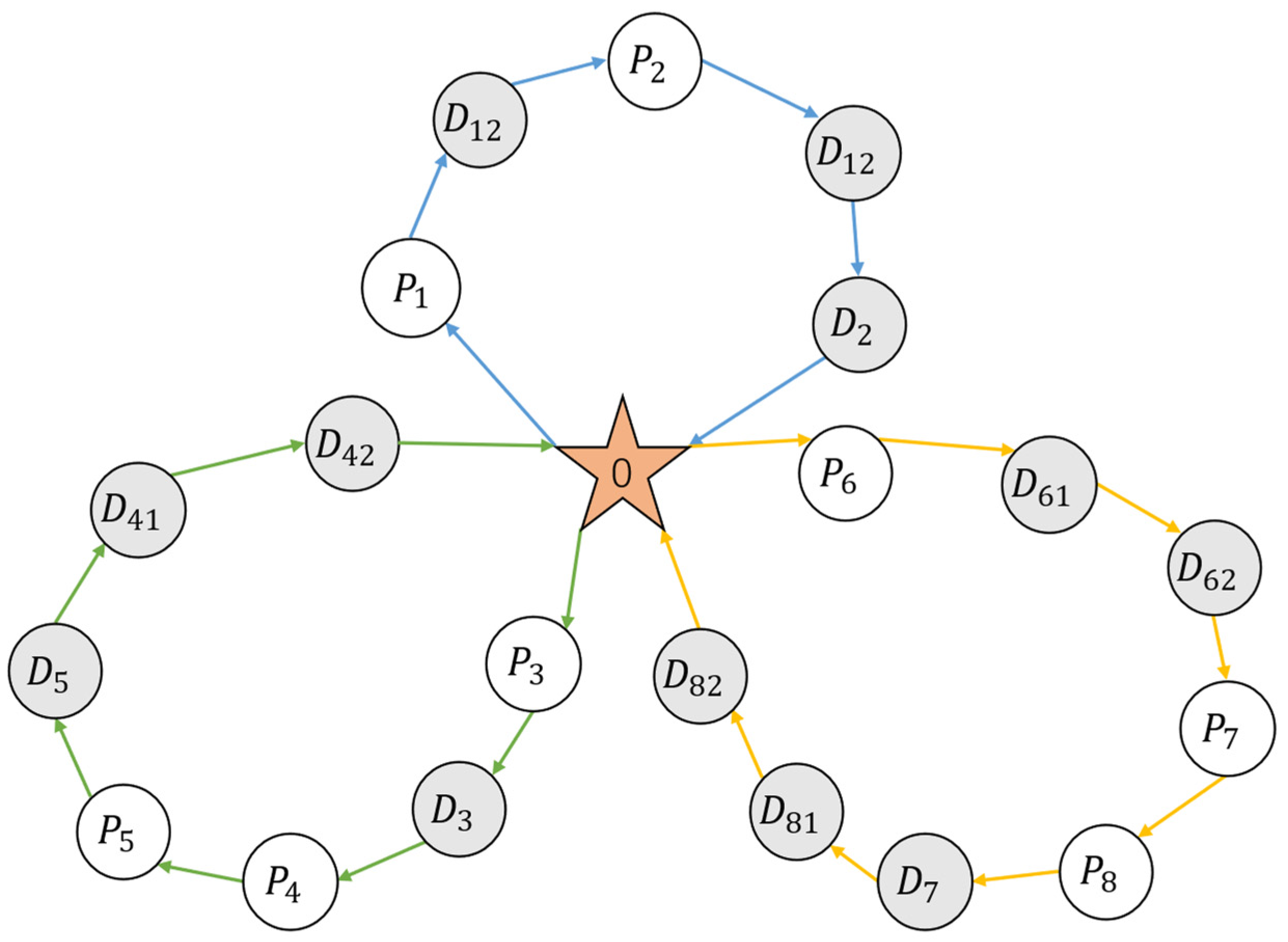
Figure 1 illustrates an example of the vehicle distribution network structure. Node $0$ denotes the depot; $P_1,\dots ,P_8$ represent pickup nodes, and $D_{11},D_{12},D_2,\dots ,D_{82}$ denote delivery nodes. For instance, $D_{11}$ and $D_{12}$ are two different delivery locations corresponding to pickup node $P_1$. The network depicts a closed-loop routing pattern for three vehicles: Vehicle 1 follows the route $0\to P_1\to D_{11}\to P_2\to D_{12}\to D_2\to 0$; Vehicle 2 follows $0\to P_3\to D_3\to P_4\to P_5\to D_5\to D_{41}\to D_{42}\to 0$; and Vehicle 3 follows $0\to P_6\to D_{61}\to D_{62}\to P_7\to P_8\to D_7\to D_{81}\to D_{82}\to 0$. These illustrate the one-to-many pickup–delivery relationships and the closed-loop routing pattern.

3.2. Model Parameters

For clarity and ease of reference, the key notations, decision variables, and parameters employed in the mathematical formulation are summarized in

Table 1. Model Parameters.

Parameter	Description
$P$	set of pickup nodes, indexed by $p$
$D$	set of delivery nodes, indexed by $d$
$N$	number of nodes
$K$	set of vehicles, indexed by $k$
$M_p$	set of item indices associated with pickup node $p$, indexed by $m$
$c_{ij}$	travel distance between node $i$ and node $j$
$L,W,H$	length, width, and height of the vehicle loading space
$Q_{max}$	maximum weight capacity of a vehicle
$V_{max}$	maximum size of the available vehicle fleet
$D_{max}$	maximum travel distance of vehicles
$l_{pm}{w}_{pm}{h}_{pm}$	length, width, and height of item $I_{pm}$
$q_{pm}$	weight of item $I_{pm}$
$f_{pm}$	fragility indicator for item $I_{pm},$ equal to 1 if the item is fragile, 0 otherwise
$M$	a sufficiently large positive constant (big-M)
$x_{ijk}$	binary variable, equal to 1 if vehicle $k$ travels directly from node $i$ to node $j$, 0 otherwise
$g_{ik}$	binary variable, equal to 1 if node $i$ is visited by vehicle $k$, 0 otherwise
$u_{ik}$	auxiliary variable representing the visit sequence number of node $i$ in the route of vehicle $k$
$x_{pmk},y_{pmk},z_{pmk}$	coordinates of the bottom-left-rear corner of item $I_{pm}$ when loaded onto vehicle $k$
$∆x_{pmk},∆y_{pmk},∆z_{pmk}$	effective dimensions of item $I_{pm}$ along the $x,y,$ and $z$ axes on vehicle $k$
$r_{pmk}$	binary orientation variable, equal to 1 if item $I_{pm}$ is rotated by 90° in the horizontal plane on vehicle $k$, and 0 otherwise.
$o_{pm,p^{\prime }{m}^{\prime }k}$	binary variable, equal to 1 if item $I_{p^{\prime }{m}^{\prime }}$ is stacked directly on top of item $I_{pm}$ on vehicle $k$, and 0 otherwise

.

3.3. Mathematical Model

3.3.1. Objective Function

The primary objective is to minimize the total travel distance across all deployed vehicles:

$$\mathit{min}f=\sum _{k\in K}\sum _{i\in N}\sum _{j\in N}{c}_{ij}{x}_{ijk}$$

(1)

3.3.2. Loading Constraint

• Fragility Constraint: If item $I_{pm}$ is fragile ($f_{pm}=1$), and item $I_{p^{\prime }{m}^{\prime }}$ is non-fragile ($f_{p^{\prime }{m}^{\prime }}=0$), then the fragile item must be placed on top:

  $$\begin{gathered} z_{pmk}>z_{p^{\prime }{m}^{\prime }k}+h_{p^{\prime }{m}^{\prime }}-M\left(2-g_{pk}-g_{p^{\prime }k}\right) \\ \forall p,p^{\prime }\in P,\forall m\in M_p,\forall m^{\prime }\in M_{p^{\prime }},\forall k\in K \end{gathered}$$

  (2)

The term $M\left(2-g_{pk}-g_{p^{\prime }k}\right)$ functions as a conditional activation mechanism for the constraint. When both item $I_{pm}$ and item $I_{p^{\prime }{m}^{\prime }}$ are assigned to the same vehicle $k$, the penalty term vanishes, strictly enforcing that the fragile item must be placed above the non-fragile one. Conversely, if either request is not served by vehicle $k$, the large constant $M$ makes the right-hand side sufficiently small, rendering the inequality redundant.

2.

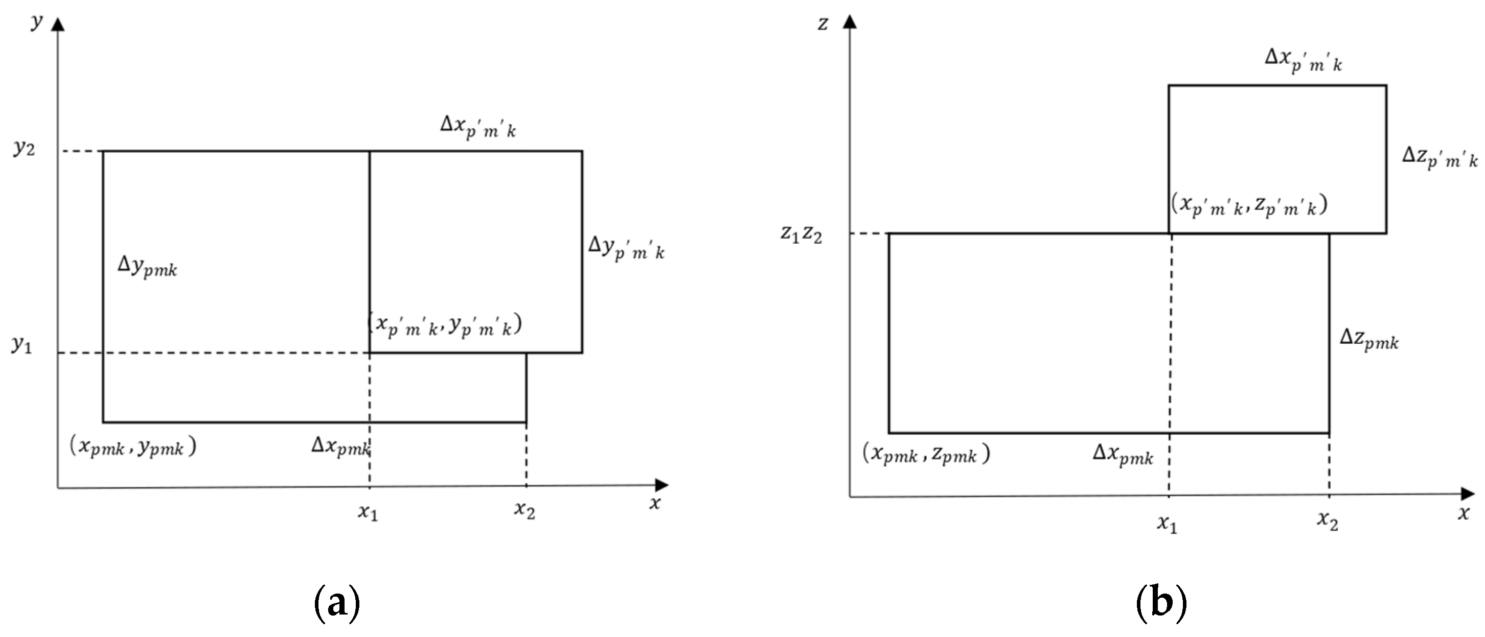
Stacking Constraint: If item $I_{p^{\prime }{m}^{\prime }}$ is stacked on top of item $I_{pm}$($o_{pm,p^{\prime }{m}^{\prime }k}=1$), then the contact area between items $I_{p^{\prime }{m}^{\prime }}$ and $I_{pm}$ must meet a certain proportion of the bottom area of each item. This constraint is calculated by computing the overlapping area of the two items’ projections on the horizontal plane. To present this more intuitively, the $xy$ and $xz$ two-dimensional projection diagrams of items $I_{pm}$ and $I_{p^{\prime }{m}^{\prime }}$ loaded on vehicle $k$ are shown in Figure 2. In these diagrams, $(x_{pmk},y_{pmk})$ and $(x_{p^{\prime }{m}^{\prime }k},y_{p^{\prime }{m}^{\prime }k})$ represent the placement coordinates of the two items:

$$x_1=max\left\{x_{pmk},x_{p^{\prime }{m}^{\prime }k}\right\},x_2=min\left\{x_{pmk}+{∆x}_{pmk},x_{p^{\prime }{m}^{\prime }k}+{∆x}_{p^{\prime }{m}^{\prime }k}\right\}$$

(3)

$$y_1=max\left\{y_{pmk},y_{p^{\prime }{m}^{\prime }k}\right\},y_2=min\left\{y_{pmk}+{∆y}_{pmk},y_{p^{\prime }{m}^{\prime }k}+{∆y}_{p^{\prime }{m}^{\prime }k}\right\}$$

(4)

$$z_1=max\left\{z_{pmk},z_{p^{\prime }{m}^{\prime }k}\right\},z_2=min\left\{z_{pmk}+{∆z}_{pmk},z_{p^{\prime }{m}^{\prime }k}+{∆z}_{p^{\prime }{m}^{\prime }k}\right\}$$

(5)

The overlap lengths in the $x$ and $y$ directions are:

$$L_x^{overlap}=max(0, x_2-x_1)$$

(6)

$$L_y^{overlap}=max(0, y_2-y_1)$$

(7)

The overlapping area $A_{ij}^{\mathrm{overlap}}$ is:

$$A_{pm,p\prime m\prime }^{overlap}=L_x^{overlap}\times L_y^{overlap}$$

(8)

The stability constraint is thus formulated as:

$$\begin{gathered} A_{pm,p^{\prime }{m}^{\prime }}^{overlap}\ge \alpha ·\left(l_{p^{\prime }{m}^{\prime }}·w_{p^{\prime }{m}^{\prime }}\right)-M·\left(1-o_{pm,p^{\prime }{m}^{\prime }}\right) \\ \forall p,p^{\prime }\in P; \forall m\in M_p; \forall m^{\prime }\in M_{p^{\prime }} \end{gathered}$$

(9)

where $\alpha \in \left(\mathrm{0,1}\right)$ is the minimum support ratio, defined as the proportion of the upper item’s base area that must be supported by the lower items. For the stacking stability constraint, the minimum support ratio was set to $\alpha =0.75$.

3.

Orientation Constraint: Items are allowed to rotate 90° within the horizontal plane. Vertical rotation is prohibited to strictly adhere to “This Way Up” constraints common in logistics, ensuring the structural integrity of fragile goods and maintaining a low center of gravity for transport stability. The projection dimensions on the coordinate axes are determined by the orientation in which the item is placed in vehicle $k$, and are specifically defined by the following formula:

$$∆x_{pmk}=\left\{\left(1-r_{pmk}\right)l_{pm}+r_{pmk}{w}_{pm}\right\}$$

(10)

$$∆y_{pmk}=\left\{\left(1-r_{pmk}\right)w_{pm}+r_{pmk}{l}_{pm}\right\}$$

(11)

$$\begin{gathered} ∆z_{pmk}=h_{pm} \\ \forall p\in P,\forall m\in M_p,\forall k\in K \end{gathered}$$

(12)

4.

Boundary Constraints: Items must be placed within the vehicle’s cargo dimensions and coordinates must be non-negative:

$$0\le x_{pmk}\le L-∆x_{pmk}$$

(13)

$$0\le y_{pmk}\le W-∆y_{pmk}$$

(14)

$$\begin{gathered} 0\le z_{pmk}\le H-∆z_{pmk} \\ \forall p\in P,\forall m\in M_p,\forall k\in K \end{gathered}$$

(15)

5.

Weight Constraint: The total weight of loaded items on any vehicle $k$ must not exceed its capacity $Q_{max}$:

$$\sum _{p\in P}\sum _{m\in M_p}{q}_{pm}·g_{pk}\le Q_{max} \forall k\in K$$

(16)

6.

Volume Constraint: The total volume of loaded items must not exceed the vehicle’s volume limit:

$$\sum _{p\in P}\sum _{m\in M_p}{l}_{pm}·w_{pm}·h_{pm}·g_{pk}\le L·W·H \forall k\in K$$

(17)

7.

Non-overlapping Constraint: Any two boxes placed in the same vehicle’s loading space must not overlap:

$$\begin{gathered} \left(x_{pmk}\ge x_{p^{\prime }{m}^{\prime }k}+∆x_{p^{\prime }{m}^{\prime }k}\right)\vee \left(x_{p^{\prime }{m}^{\prime }k}\ge x_{pmk}+∆x_{pmk}\right)\vee \\ \left(y_{pmk}\ge y_{p^{\prime }{m}^{\prime }k}+∆y_{p^{\prime }{m}^{\prime }k}\right)\vee \left(y_{p^{\prime }{m}^{\prime }k}\ge y_{pmk}+∆y_{pmk}\right)\vee \\ \left(z_{pmk}\ge z_{p^{\prime }{m}^{\prime }k}+∆z_{p^{\prime }{m}^{\prime }k}\right)\vee \left(z_{p^{\prime }{m}^{\prime }k}\ge z_{pmk}+∆z_{pmk}\right) \\ \forall p,p^{\prime }\in P,\forall m\in M_p,\forall m^{\prime }\in M_{p^{\prime }},\forall k\in K \end{gathered}$$

(18)

3.3.3. Route Constraint

• Node Visit Constraint: Each customer node must be served by only one vehicle once.

  $$\sum _{k\in K}\sum _{j\in N}{x}_{ijk}=1 \forall i\in P\cup D$$

  (19)
• Depot Constraints: Every vehicle route must start and end at the depot:

  $$\sum _{j\in P}{x}_{0jk}\le 1 \forall k\in K$$

  (20)

  $$\sum _{i\in D}{x}_{i0k}\le 1 \forall k\in K$$

  (21)
• Flow Balance Constraint: After a vehicle services a node, it must leave the node.

  $$\sum _{i\in N}{x}_{ijk}=g_{jk} \forall k\in K,\forall j\in N$$

  (22)

  $$\sum _{j\in N}{x}_{ijk}=g_{ik} \forall k\in K,\forall i\in N$$

  (23)
• Pickup-Delivery Sequence Constraint: This constraint ensures the precedence relationship between pickup and delivery operations. Specifically, for any delivery node $d\in D$, let $p\left(d\right)\in P$ denote its associated pickup node. If vehicle $k$ serves this request, the pickup node must be visited before the delivery node.

  $$u_{p\left(d\right),k}\le u_{d,k}-1+M\left(2-g_{p\left(d\right),k}-g_{d,k}\right) \forall d\in D,\forall k\in K$$

  (24)

This constraint ensures that when $g_{p\left(d\right),k}=1$ and $g_{d,k}=1$, we have $u_{p\left(d\right),k}<u_{d,k}$.

5.

Subtour Elimination Constraint: Ensures that the order of nodes visited by a vehicle is strictly increasing along its route, eliminating any possible subtours.

$$u_{ik}-u_{jk}+\left|N\right|·x_{ijk}\le \left|N\right|-1 \forall i,j\in P\cup D,k\in K$$

(25)

6.

One-to-Many Vehicle Consistency Constraint: All delivery nodes corresponding to the same pickup node must be serviced by the same vehicle.

$$g_{p\left(d\right),k}=g_{d,k} \forall d\in D,\forall k\in K$$

(26)

7.

Vehicle Travel Distance Constraint: The travel distance of the vehicle cannot exceed the maximum allowed travel distance.

$$\sum _{i\in N}\sum _{j\in N}{c}_{ij}{x}_{ijk}\le D_{max} \forall k\in K$$

(27)

8.

Vehicle Quantity Constraint: The number of vehicles used cannot exceed the maximum vehicle quantity.

$$\sum _{k\in K}\sum _{j\in P}{x}_{0jk}\le V_{max}$$

(28)

4. Methods

To address the one-to-many 3L-PDVRP, this paper proposes a deeply coupled HGA. The algorithm adopts a grouping-based chromosome representation for vehicle routes and embeds a three-dimensional loading verification module into the evolutionary search. In each generation, candidate routing solutions are evaluated by a route-and-loading procedure that checks loading feasibility, attempts repair when infeasibilities occur, and incorporates loading outcomes into the fitness value. In this way, routing optimization and loading verification interact in a closed-loop manner.

In Algorithm 1, the function $EvaluateRouteAndLoading(\cdot )$ is the key component that couples routing optimization with three-dimensional loading verification. It calls the loading algorithm described in Section 4.3 to check the feasibility of the generated routes and performs loading-aware repair or penalization based on the outcomes.

Algorithm 1: Hybrid Genetic Algorithm

Input: Population size $P$, Maximum generations $G$, Mutation rate $p_m$, Crossover rate $p_c$, Elitism count $E$ Output: Best solution $S_{best}$

1.   $P_{current}\leftarrow$ InitializePopulation($P$) 2.   EvaluatePopulation($P_{current}$) 3.   $S_{best} \leftarrow$ GetFittest($P_{current}$) 4.   for $g= 1$ to $G$ do 5.      $P_{new}$ $\leftarrow \mathrm{\varnothing }$ 6.      //Elitism Strategy 7.      for $i= 1$ to $E$ do 8.           $P_{new}$. Add (GetFittest($P_{current}$, $i$)) 9.      end for 10.    //Evolutionary process in current generation 11.    while $\left|P_{new}\right|$ < $P$ do 12.         ${parent}_1$, ${parent}_2\leftarrow$ SelectParents($P_{current}$) 13.         //Crossover 14.         if rand() < $p_c$then 15.                ${child}_1$, ${child}_2\leftarrow$ Crossover(${parent}_1$, ${parent}_2$) 16.         else 17.                ${child}_1$ $\leftarrow$ ${parent}_1$ 18.                ${child}_2\leftarrow {parent}_2$ 19.         end if 20.         //Adaptive route-reconstruction mutation with hybrid insertion 21.         AdaptiveMutation(${child}_1, p_m$, $g$, $G$) 22.         AdaptiveMutation(${child}_2, p_m$, $g$, $G$) 23.         // Deeply coupled three-dimensional loading verification and feedback repair 24.         if not IsValidLoading(${child}_1$) then 25.                ${child}_1\leftarrow$ LoadingAwareRepair(${child}_1$) 26.         end if 27.         if not IsValidLoading(${child}_2$) then 28.                ${child}_2\leftarrow$ LoadingAwareRepair(${child}_2$) 29.         end if 30.         //Fitness evaluation with loading penalties 31.         EvaluateRouteAndLoading(${child}_1$) 32.         EvaluateRouteAndLoading(${child}_2$) 33.         $P_{new}$.add(${child}_1$, ${child}_2$) 34.    end while 35.    $P_{current}$ $\leftarrow$ $P_{new}$ 36.    $S_{current}\leftarrow$ GetFittest($P_{current}$) 37.    if Fitness($S_{current}$) > Fitness($S_{best})$ then 38.         $S_{best}\leftarrow$ $S_{current}$ 39.    end if 40. end for 41. return $S_{best}$

4.1. Overall Framework Design

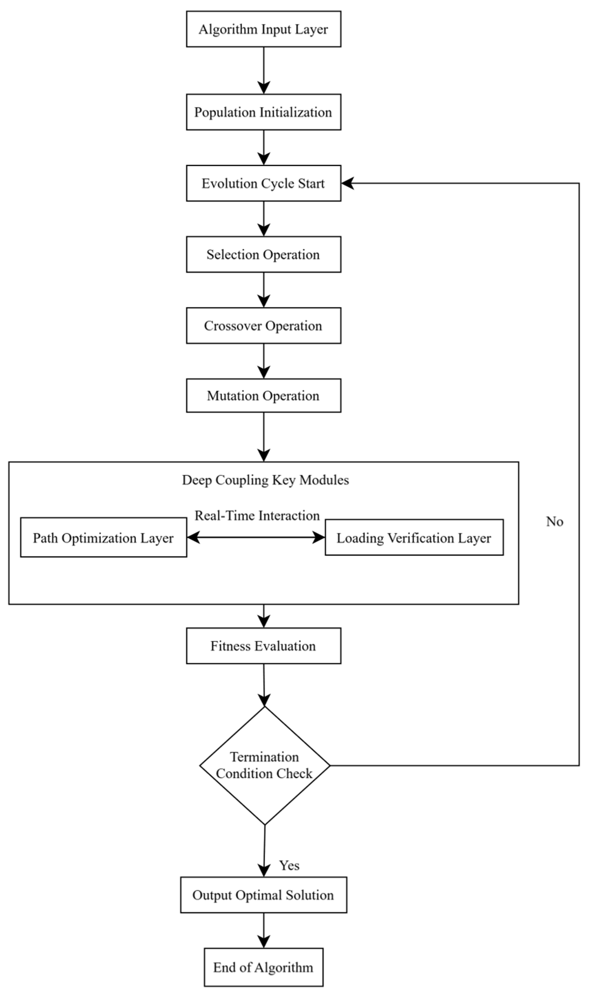
The core concept of this algorithm is based on dynamic interaction between route optimization and loading verification. Conventional methods typically address these two subproblems separately, often leading to solutions that are impractical during actual loading. The proposed algorithm incorporates dynamic loading verification at each critical stage of genetic evolution, ensuring that the resulting delivery plans are both route efficient and operationally feasible.

The algorithmic framework is shown in Figure 3, with the overall process consisting of:

Outer-layer route optimization: A Grouping Genetic Algorithm (GGA) framework is used, where the population is divided into subpopulations that evolve independently, exploring the optimal route space.

Inner-layer loading verification: Real-time loading feasibility checks are performed to ensure that each generated route solution satisfies the 3D loading constraints. Loading verification is triggered whenever a new route is generated; if loading is infeasible, the route is adjusted through fitness penalties and route repair mechanisms.

Deep Coupling Mechanism: Load feasibility acts as the core indicator for fitness evaluation. Route optimization and load verification are tightly interwoven during fitness calculation, thereby forming a closed-loop feedback mechanism.

4.2. Route Optimization Algorithm

The route construction algorithm uses a hybrid genetic algorithm based on the GGA framework. This approach integrates route optimization with 3D loading verification, using outer-layer genetic operations to explore the route space and embedding inner-layer loading checks during fitness evaluation to ensure the practical feasibility of solutions.

4.2.1. Chromosome Encoding and Population Initialization

A grouping-based encoding strategy is used. Each chromosome represents a complete delivery plan with multiple genes. As illustrated in Figure 4, a single gene represents the complete travel route of a delivery vehicle, encoded so that the depot serves as both the starting and ending nodes, with visits to pickup nodes and their corresponding delivery nodes occurring sequentially. This coding approach inherently satisfies the constraint that pickup nodes must be visited before their corresponding delivery nodes.

This encoding method has three advantages: first, it naturally captures the grouping characteristics of vehicle routing problems, since each gene represents a group of customers assigned to the same vehicle; second, the variable-length chromosome design allows different numbers of vehicles to be used, which is suitable for problems with flexible fleet sizes; third, the encoding structure ensures that pickup nodes are visited before their corresponding delivery nodes.

Population initialization uses an incremental construction method to generate diverse initial feasible solutions. The steps are as follows:

• During initialization, all pickup nodes are randomly sorted;
• Each pickup node and its associated delivery node are sequentially inserted into the current route structure;
• During insertion, a greedy algorithm selects the insertion position that minimizes the cost increase for each pickup node;
• If the existing route cannot accommodate a new pickup node, a new vehicle route is created.

This method guarantees the feasibility of the initial solutions while ensuring population diversity through random sorting.

4.2.2. Fitness Function

The fitness function uses a weighted summation method, combining route length and constraint violation penalties. The core calculation involves subtracting the total route cost from a fixed baseline, so that solutions with shorter routes and fewer constraint violations have higher fitness. The total route cost consists of the driving distance and constraint violation penalties. The penalty components include penalties for unserved customers and loading infeasibility. The unserved customer penalty is calculated based on the number of unserved customers, ensuring the algorithm prioritizes fulfilling all service demands. The loading infeasibility penalty carries a high weight, forcing the algorithm to seek feasible solutions that satisfy the three-dimensional loading constraints.

The mathematical expression for the fitness function is provided as follows:

$$F=B-\left(S+\lambda ·P_{unserved}+\mu ·P_{loading}\right)$$

(29)

where $B$ is a fixed baseline value, $S$ denotes the total distance traveled by the vehicle, and $\lambda$ and $\mu$ are penalty coefficients corresponding to penalties for failing to serve customers and for loading infeasibility, respectively. The values were fixed at $\lambda =1000$ and $\mu =\mathrm{10,000}$ to establish a strict hierarchy of objectives: loading feasibility > service completeness > distance minimization.

4.2.3. Genetic Operator Design

Selection operation: A strategy combining tournament selection and elite retention is used. Tournament selection randomly selects a fixed number of individuals, choosing the highest-fitness ones as parents. The elite retention strategy preserves the optimal individuals from the current generation for the next generation.

Crossover operation: A grouping-preserving crossover algorithm is used. Gene fragments are selected from the parent generation and inserted into the offspring generation. Conflicting pickup/delivery nodes are removed from the offspring generation, and the chromosome is repaired. The repair process uses a greedy insertion strategy, reinserting unassigned customers into the route.

Mutation operation: A route reconstruction mutation is used. Non-empty genes are randomly selected, and their customer nodes are cleared, then redistributed using a hybrid insertion strategy. The mutation probability uses an adaptive mechanism, maintaining a higher mutation rate during early evolution to enhance exploration and gradually decreasing it later to strengthen local search.

4.2.4. Hybrid Insertion Strategy

The hybrid insertion strategy dynamically adjusts the ratio of greedy to regret insertion based on the evolutionary stage. The greedy insertion algorithm calculates the cost of all feasible insertion positions for each pending customer and selects the position with the smallest cost increase. The regret insertion algorithm introduces a forward-looking mechanism, considering the current insertion cost and evaluating the impact of decisions on subsequent operations. The Regret-2 algorithm calculates the cost difference between the optimal and suboptimal insertion positions. The Regret-3 algorithm further considers the cost relationships among the top three optimal insertion positions. During the early evolutionary phase, regret insertion predominates to enhance global exploration. In the later evolutionary phase, the proportion of greedy insertion increases to accelerate convergence to high-quality solutions.

4.3. Three-Dimensional Loading Algorithm

The three-dimensional loading algorithm ensures cargo meets spatial constraints within the vehicle compartment through dynamic simulation, maximum space partitioning, multi-strategy box placement, and strict constraint management. This algorithm collaborates with the route construction algorithm to ensure the practical feasibility of delivery solutions.

The spatial partitioning algorithm uses the maximum space method for three-dimensional space division, as shown in Figure 5. After placing a box, the algorithm generates new residual spaces in three orthogonal directions: rightward along the length, rearward along the width, and upward along the height. After partitioning, overlapping or adjacent spatial regions are automatically merged to reduce fragmentation and enhance space utilization.

The box placement follows a multi-stage strategy: The corner-priority strategy places boxes tightly against the corners of the cargo hold to ensure stability; the edge-secondary strategy places boxes along the hold’s edges to maintain clear passageways; the top-placement strategy stacks boxes atop existing ones to utilize vertical space; the center-placement strategy places boxes at the spatial center to balance weight distribution. Each strategy includes 90° horizontal rotation optimization.

Algorithm Execution Steps

Step 1: Initialize the loading status. Let the set of goods currently in the carriage be denoted as $B$ (initially empty), the set of remaining available space as $F$ (initially the entire carriage space), and the set of goods awaiting loading for the current customer as $I_i$. Initialize the current customer’s loading plan as $S_i=\mathrm{\varnothing }$.

Step 2: Generate candidate loading sequences. Implement a multi-sorting strategy to rank the goods within $I_i$ according to descending volume, descending base area, ascending fragility, and descending height. This yields four candidate loading sequences $C=\{{seq}_1,{seq}_2,{seq}_3,{seq}_4\}$, providing diverse initial schemes for subsequent loading attempts.

Step 3: Sequential loading execution. From the candidate sequence set $C$, the current sequence ${seq}_k$ is selected. For each cargo item $I_{im}$ in this sequence, loading operations are performed sequentially using a four-stage placement strategy (corner priority, edge priority, top placement, center placement), combined with 90-degree rotation optimization. If a cargo item is successfully placed, the loading plan $S_i$ and the remaining space set $F$ are updated. If any cargo item in the current sequence cannot be successfully placed, proceed to Step 5.

Step 4: Stability verification. Perform stability verification on the successfully loaded scheme $S_i$, checking the compliance with support area constraints and basic stability requirements. If all constraints are satisfied, proceed to Step 6; otherwise, proceed to Step 5.

Step 5: Sequence switching processing. Remove the current sequence ${\mathrm{s}\mathrm{e}\mathrm{q}}_k$ from the candidate set $C$. If $C\ne \mathrm{\varnothing }$, return to Step 3 to select a new candidate sequence and retry. Otherwise, determine that the current customer’s goods loading has failed, output $S_i=\varnothing$, and terminate the algorithm.

Step 6: Status update and output. Merge the successfully loaded cargo collection into the global cargo collection, update $B$ to $B\cup S_i$, and output the complete loading scheme $S_i$. The updated spatial status $F$ provides a basis for the subsequent loading of customer goods.

In the HGA, Algorithm 2 is called within $EvaluateRouteAndLoading(\cdot )$ whenever the loading feasibility of a given route or group of routes needs to be checked.

Algorithm 2: 3D Cargo Loading Algorithm

Input: Current customer items $I_i$, Global items set $B$, Remaining space $F.$ Output: Loading scheme $S_i$, Updated space state $F$, Status (SUCCESS/FAILED).

1.   Initialize $S_i$ ← $\varnothing$ 2.   $se{q}_1$ ← Sort($I_i$, volume, DESC) 3.   $se{q}_2$ ← Sort($I_i$, base area, DESC) 4.   $se{q}_3$ ← Sort($I_i$, fragility, ASC) 5.   $se{q}_4$ ← Sort($I_i$, height, DESC) 6.   $C$ ← Merge($se{q}_1, se{q}_2$, $se{q}_3$, $se{q}_4$) 7.   while $C \ne \varnothing$ do 8.       $se{q}_k$← SelectNextSequence($C$) 9.       success ← true 10.     ${temp}_F$ ← $F$ 11.     ${temp}_{S_i}$ ← $\varnothing$ 12.     for each $item \in se{q}_k$ do 13.           position_found ← false 14.           candidate_positions ← GenerateCandidatePositions(${temp}_F$) 15.           for each position $\in$ candidate_positions do 16.                  for each orientation ∈ {original, 90° rotation} do 17.                         if IsValidPosition(item, position, orientation, ${temp}_F$, $B$) then 18.                               ${temp}_{S_i}$ ←${temp}_{S_i}$ $\cup$ {(item, position)} 19.                               ${temp}_F$ ← UpdateSpace(${temp}_F$, item, position, orientation) 20.                               position_found ← true 21.                               break 22.                         end if 23.                  end for 24.                  if position_found then 25.                         break 26.                  end if 27.           end for 28.           if not position_found then 29.                  success ← false 30.                  break 31.           end if 32.    end for 33.    if success then 34.           if CheckSupportArea(${temp}_{S_i}$) and 35.                  CheckStability(${temp}_{S_i}$) then 36.                  $S_i$ ← ${temp}_{S_i}$ 37.                  $F$← ${temp}_F$ 38.                  $B$ ← $B$ ∪ $S_i$ 39.                  return ($S_i$, $F$, SUCCESS) 40.           end if 41.    end if 42.    $C$ ←$C$ \ {$se{q}_k$} 43. end while 44. return ($\varnothing$, $F$, FAILED)

4.4. Summary of Algorithm Innovations

The core innovation of this algorithm lies in its deep coupling mechanism between route optimization and load verification. Specifically, load verification is integrated as part of the fitness evaluation at every stage of route optimization, ensuring that generated solutions simultaneously satisfy both route and load constraints.

• Synergy between Route Optimization and Loading Verification: Instead of optimizing routes and checking loading feasibility in separate stages, the proposed HGA integrates the loading module into the fitness evaluation. As a result, routing decisions are guided toward patterns that are both efficient in terms of travel distance and compatible with realistic three-dimensional loading constraints.
• Real-time feedback mechanism for loading verification: After route crossings and mutation operations, loading verification is performed. If verification fails, the solution is not discarded immediately; instead, the route recommendation is adjusted through the feedback mechanism. After verification failure, the route is optimized using sequence change repair strategies to ensure compliance with loading constraints. This creates a closed-loop feedback mechanism between route optimization and loading verification repair. This closed-loop feedback enables interaction between route optimization and loading verification, enhancing the algorithm’s overall optimization capability.
• Flexible yet structured encoding: The grouping-based encoding and hybrid insertion strategy allow the algorithm to handle different numbers of vehicles and complex one-to-many pickup–delivery patterns while preserving precedence and capacity constraints.

Through these mechanisms, the proposed algorithm is able to address the one-to-many 3L-PDVRP in a way that jointly considers routing efficiency and three-dimensional loading feasibility, providing a practically meaningful solution approach for complex distribution operations.

5. Experiments

5.1. Experimental Environment and Test Data

The experiment was conducted in a standard computing environment using a PC with the following hardware: 13th Gen Intel(R) Core (TM) i5-13500H processor (2.60 GHz) and 16 GB of RAM. The method was implemented in Java without the use of any external commercial solvers or third-party optimization libraries. The algorithm parameters were determined through preliminary experiments: a population size of 20, a mutation rate of 0.15, a crossover rate of 0.85, elite retention of 2 individuals, a tournament size of 3, and a maximum of 100 generations. 54 standard test instances publicly available from Männel et al. (2016) [29] were adopted, covering three node distribution patterns and three customer scales, forming a comprehensive test matrix.

Table 2. Overview of the 54 new 3L-PDP benchmark instances.

Number of Requests	2 Boxes per Request on Average			3 Boxes per Request on Average			Total
	CLUS	CPCD	RAND	CLUS	CPCD	RAND
50	5	5	5	5	5	5	30
75	3	3	3	3	3	3	18
100	1	1	1	1	1	1	6

details the data distribution characteristics of the test instances. Here, “CLUS” indicates that the vertices in the instances exhibit a clustered distribution, forming several clusters; “CPCD” has a vertex distribution similar to “CLUS”, with the distinction that each cluster contains only either pickup nodes or delivery nodes; “RAND” indicates that the vertices are randomly and uniformly distributed within a rectangular plane.

The vehicle parameters are as follows: cargo compartment dimensions of 6 m × 2.5 m × 3 m, rated payload capacity of 45,000 kg, and maximum operational range of 1236 km. The vehicle specifications are kept fixed and identical to those defined in the standard benchmark instances.

Construction of One-to-Many 3L-PDVRP Instances

The original benchmark set in Männel et al. [29] is defined for a one-to-one 3L-PDP, in which each pickup request is associated with a single delivery node. To evaluate the proposed algorithm in the one-to-many setting considered in this paper, these instances were extended as follows:

For each pickup node $p$, the associated boxes are partitioned into several subsets, and each subset is assigned to one delivery node. The coordinates of the new delivery nodes are generated by perturbing the original delivery location within a small neighborhood. All delivery nodes originating from the same pickup node must be served by the same vehicle, and the total volume and weight of the boxes remain unchanged relative to the original request.

This transformation yields a set of one-to-many 3L-PDVRP instances that preserve the spatial patterns and demand characteristics of the original benchmarks while explicitly modeling one-to-many pickup delivery relationships. These transformed instances are used in all subsequent experiments.

5.2. Multi-Scale Instance Solving

To evaluate algorithm performance, this paper employs the large neighborhood search (LNS) method proposed by Männel et al. [29] as a comparative algorithm. It is applied to contrast with the proposed HGA algorithm. Both algorithms share identical instance data and evaluation functions, utilizing consistent parameter settings. Test results were averaged over ten computations, as shown in

Table 3. Small-Scale Instance Solving Results.

Instance	Average Route Length (km)		Average Loading Rate (%)		Average Number of Vehicles
	HGA	LNS	HGA	LNS	HGA	LNS
050_CLUS_2_1	1241.48	1337.37	86.32	85.21	4	4
050_CLUS_2_2	1175.24	1225.44	81.91	82.38	4	4
050_CLUS_2_3	1237.88	1319.43	85.17	81.94	4	4
050_CLUS_2_4	1211.36	1422.37	82.73	81.34	4	4
050_CLUS_2_5	1309.91	1508.56	88.54	85.49	4	5
050_CPCD_2_1	1402.36	1523.12	77.28	80.01	5	4
050_CPCD_2_2	1338.92	1462.28	86.12	83.27	4	4
050_CPCD_2_3	1321.47	1626.46	88.75	86.57	4	5
050_CPCD_2_4	1383.29	1628.28	82.93	83.28	4	5
050_CPCD_2_5	1398.23	1692.55	83.63	82.16	4	5
050_RAND_2_1	1326.71	1731.28	79.45	77.28	4	5
050_RAND_2_2	1298.47	1522.35	80.32	76.18	4	4
050_RAND_2_3	1307.38	1517.26	82.36	80.92	4	4
050_RAND_2_4	1472.46	1576.33	82.13	79.27	4	4
050_RAND_2_5	1389.53	1512.78	80.92	80.11	4	4
Avg	1320.98	1507.06	83.24	81.69	4.07	4.33
050_CLUS_3_1	1432.84	1702.92	80.45	80.06	4	4
050_CLUS_3_2	1452.36	1763.82	82.48	79.41	5	4
050_CLUS_3_3	1384.29	1728.55	85.29	81.98	4	5
050_CLUS_3_4	1407.63	1823.21	82.97	82.13	5	4
050_CLUS_3_5	1421.11	1752.29	83.86	79.58	5	5
050_CPCD_3_1	1627.39	1839.43	80.31	76.13	4	5
050_CPCD_3_2	1633.94	1827.39	84.35	80.93	4	5
050_CPCD_3_3	1712.83	1973.47	81.23	78.76	4	5
050_CPCD_3_4	1623.54	1911.58	78.36	75.34	5	5
050_CPCD_3_5	1673.82	1855.53	84.78	80.46	5	5
050_RAND_3_1	1562.83	1946.05	82.67	80.23	4	5
050_RAND_3_2	1562.73	1731.79	83.15	81.02	4	4
050_RAND_3_3	1527.98	1813.45	84.54	80.14	5	4
050_RAND_3_4	1496.46	1648.49	82.73	80.36	4	5
050_RAND_3_5	1548.22	1612.78	79.92	77.83	5	5
Avg	1537.86	1795.38	82.47	79.62	4.47	4.67

and

Table 4. Large-Scale Instance Solving Results.

Instance	Average Route Length (km)		Average Loading Rate (%)		Average Number of Vehicles
	HGA	LNS	HGA	LNS	HGA	LNS
075_CLUS_2_1	1620.43	1932.36	79.74	78.92	6	6
075_CLUS_2_2	1642.57	1927.44	82.11	79.41	6	6
075_CLUS_2_3	1617.53	2053.87	76.83	77.84	6	6
075_CPCD_2_1	2276.92	2431.76	79.44	77.93	6	7
075_CPCD_2_2	2107.63	2492.43	76.27	75.06	6	7
075_CPCD_2_3	2298.65	2563.13	83.92	80.1	7	7
075_RAND_2_1	2020.55	2343.84	78.46	78.08	6	6
075_RAND_2_2	2043.35	2392.92	82.13	79.63	6	6
075_RAND_2_3	2058.12	2301.46	77.51	76.12	6	6
Avg	1965.08	2271.02	79.60	78.12	6.11	6.33
075_CLUS_3_1	1782.28	2017.53	86.74	83.55	6	6
075_CLUS_3_2	1728.92	1998.53	81.23	80.04	6	6
075_CLUS_3_3	1801.61	2243.54	79.76	75.51	6	6
075_CPCD_3_1	2482.48	2809.25	82.34	79.96	7	7
075_CPCD_3_2	2473.97	2767.16	85.63	82.47	7	6
075_CPCD_3_3	2397.73	2813.82	89.58	86.28	6	7
075_RAND_3_1	2192.39	2372.18	80.11	78.89	6	6
075_RAND_3_2	2264.33	2391.31	81.38	77.37	6	6
075_RAND_3_3	2183.45	2417.06	82.63	80.94	6	6
Avg	2145.24	2425.60	83.27	80.56	6.22	6.22
100_CLUS_2_1	4196.04	4518.25	84.55	81.62	8	8
100_CPCD_2_1	4632.45	4953.05	85.12	83.99	8	8
100_RAND_2_1	4482.93	4613.32	86.06	84.85	8	8
Avg	4437.14	4694.87	85.24	83.49	8	8
100_CLUS_3_1	4238.82	4512.59	86.45	83.18	8	8
100_CPCD_3_1	4711.37	4996.74	83.24	80.73	9	9
100_RAND_3_1	4372.12	4704.76	84.91	81.47	8	9
Avg	4440.77	4738.03	84.87	81.79	8.33	8.67

. The results obtained from the 10 independent runs demonstrate the robustness of the proposed HGA. The variations in the final objective values are relatively small, indicating consistent convergence behavior. These tables present the overall performance of the proposed HGA and LNS algorithms in each case study, including average route length, average number of vehicles, and spatial utilization.

To quantify the improvements of the proposed deeply coupled HGA over the baseline LNS algorithm, we define the optimization gaps for both route length and loading rate. The gaps are calculated as follows:

$${Gap}_{dist}={\displaystyle \frac{{ARL}_{LNS}-{ARL}_{HGA}}{{ARL}_{LNS}}}\times 100\%$$

(30)

$${Gap}_{rate}={\displaystyle \frac{{ALR}_{HGA}-{ALR}_{LNS}}{{ALR}_{LNS}}}\times 100\%$$

(31)

where $ARL$ and $ALR$ represent the average route length and average loading rate. For both metrics, a positive gap value indicates a superior performance of the proposed HGA over the LNS baseline.

As shown in Table 3 and Table 4, the HGA algorithm demonstrates robust computational performance across diverse customer scale scenarios. As customer scale increases, both route length and vehicle utilization show reasonable growth. Compared to the LNS algorithm, the HGA algorithm achieves shorter average route lengths and higher loading rates in these cases.

Figure 6 and Figure 7 illustrate the comparison of average route lengths for small-scale and large-scale instances, respectively. As shown in both figures, the proposed HGA consistently produces shorter route lengths compared to the LNS algorithm across different problem scales, demonstrating its superior capability in optimizing travel distance.

Figure 8 and Figure 9 depict the trends of average loading rate and average number of vehicles for small-scale and large-scale instances, respectively. The difference in the number of vehicles between HGA and LNS is relatively small, although HGA sometimes uses slightly fewer vehicles. The loading rate curves show that HGA generally achieves higher loading rates than LNS and maintains this advantage as the customer scale increases.

To visually analyze the solution distribution, Figure 10 presents statistical box plots comparing the average route lengths of HGA and LNS across different scales, incorporating discrete data points to show specific solution distributions. As shown in Figure 10, the proposed HGA consistently maintains lower median and mean route lengths compared to LNS across all three customer scales. Specifically, HGA reduces the average route length by 13.43% in the 50-customer instances, 12.48% in the 75-customer instances, and 5.88% in the 100-customer instances. On average, the proposed HGA achieves a 10.60% reduction in total travel distance compared to the LNS baseline.

Figure 11 compares the performance of the two algorithms regarding average loading rates. As illustrated in Figure 11, HGA achieves higher median and mean loading rates across all scales. Quantitatively, relative to LNS, the HGA improves the loading rate by 2.72% for the 50-customer instances, 2.64% for the 75-customer instances, and 2.92% for the 100-customer instances. On average, the proposed HGA yields a 2.76% relative improvement in loading rate compared to the LNS benchmark.

Table 5. Comparison of the Average CPU Time.

Instance	HGA Average CPU Time (s)	LNS Average CPU Time (s)
50	1724	1552
75	2586	2279
100	3467	3164

compares the average CPU time of the two algorithms across different scales. The HGA consumes more time than the LNS baseline. This reflects the computational cost associated with the population-based evolution and the 3D loading checks. The proposed HGA achieves improved solution quality with a moderate increase in computational effort, demonstrating its practical applicability.

Taken together, the tabular and graphical results indicate that the proposed HGA outperforms the LNS algorithm in terms of route optimization and loading efficiency on the extended one-to-many 3L-PDVRP benchmarks.

5.3. Convergence Characteristic Analysis

The convergence processes for different-scale cases were tracked, resulting in the convergence curves shown in Figure 12. The horizontal axis represents the number of generations, and the vertical axis represents the total travel distance. The 50-customer case converged in about 18 generations, the 75-customer case in about 25 generations, and the 100-customer case in about 34 generations. All cases showed rapid initial improvement followed by stable late-stage optimization, demonstrating the algorithm’s strong global search capability and convergence stability. The convergence curve shows a stepwise decline, illustrating the breakthrough improvement of the genetic algorithm during optimization. In the early stages, the algorithm rapidly reduces the objective function value through global search; in the middle stages, it performs a fine-grained search near local optima; and in the late stages, it enters a stable state where the objective function value remains largely unchanged.

Table 6. Convergence Efficiency Analysis.

Customer Scale	Initial Distance (km)	Final Distance (km)	Convergence Generations	Improvement Count
50	2214.80	1429.42	18	9
75	4148.37	2055.16	25	12
100	8849.95	4438.96	34	22

summarizes the optimization results for different customer scales and test case sizes, including initial distance, final distance, convergence order, and number of improvements. This reflects the algorithm’s convergence efficiency across different scales. Figure 13 shows a convergence efficiency analysis for test cases of varying scales. As the customer scale increases, the number of generations required for convergence grows moderately, but the algorithm still finds high-quality solutions within reasonable computational effort. These results suggest that the proposed algorithm maintains good robustness and scalability as the problem size grows.

5.4. Case Study and Load Variation Analysis

Using the 50-customer CLUS case study (050_CLUS_2_1) for in-depth analysis, the vehicle service outcomes are shown in

Table 7. Vehicle Service Results in the Instance.

Vehicle ID	Number of Customers	Pickup/Delivery Items	Travel Distance (km)
1	30	19	287.2
2	45	32	425.4
3	38	25	325.2
4	46	30	403.7

, and the vehicle routes in

Table 8. Driving Routes of Vehicles in the Example.

Vehicle ID	Vehicle Route	Travel Distance (km)
1	0 → 30 → 50 → 30,000 → 50,000 → 26 → 33 → 16 → 33,000 → 16,000 → 9 → 16,001 → 30,001 → 45 → 45,000 → 9000 → 9001 → 9002 → 49 → 49,000 → 49,001 → 26,000 → 43 → 40 → 43,000 → 43,001 → 43,002 → 40,000 → 1 → 1000 → 1001 → 0	287.2
2	0 → 38 → 27 → 47 → 8 → 8000 → 27,000 → 27,001 → 8001 → 8002 → 35 → 14 → 2 → 15 → 22 → 14,000 → 14,001 → 14,002 → 47,000 → 38,000 → 31 → 3 → 22,000 → 22,001 → 22,002 → 31,000 → 31,001 → 38,001 → 3000 → 3001 → 3002 → 13 → 34 → 2000 → 35,000 → 35,001 → 2001 → 34,000 → 34,001 → 34,002 → 13,000 → 13,001 → 13,002 → 15,000 → 15,001 → 47,001 → 0	425.4
3	0 → 17 → 23 → 18 → 53 → 23,000 → 11 → 17,000 → 11,000 → 53,000 → 17,001 → 18,000 → 18,001 → 18,002 → 42 → 4 → 42,000 → 12 → 48 → 4000 → 5 → 48,000 → 32 → 32,000 → 32,001 → 39 → 51 → 12,000 → 32,002 → 5000 → 39,000 → 5001 → 48,001 → 4001 → 4002 → 51,000 → 51,001 → 51,002 → 42,001 → 0	325.2
4	0 → 10 → 25 → 6 → 36 → 19 → 36,000 → 19,000 → 7 → 19,001 → 10,000 → 20 → 10,001 → 7000 → 7001 → 7002 → 6000 → 25,000 → 21 → 29 → 24 → 52 → 52,000 → 24,000 → 29,000 → 29,001 → 29,002 → 24,001 → 21,000 → 37 → 46 → 46,000 → 46,001 → 21,001 → 37,000 → 37,001 → 41 → 20,000 → 20,001 → 44 → 28 → 41,000 → 28,000 → 44,000 → 44,001 → 28,001 → 41,001 → 0	403.7

. The optimal solution from the algorithm has a total travel distance of 1341.5 km, using four delivery vehicles. Each vehicle shows a balanced task allocation across customer count, cargo handling volume, loading rate, and travel distance, reflecting the algorithm’s effectiveness in route optimization and load balancing.

The actual routes are illustrated in Figure 14. All vehicle routes form closed loops starting from and returning to the depot. The visiting sequences strictly respect the one-to-many pickup–delivery structure: each pickup node is visited before all its associated delivery nodes, ensuring the feasibility of the loading and unloading operations.

In terms of load distribution, Vehicle 2 travels the longest distance, accounting for 29.5% of the total distance, and serves the largest number of customers. Its maximum loading rate during operation reaches 96.14%. In contrast, Vehicle 1 has the shortest travel distance and serves the fewest customers. The observed differences are mainly due to the non-uniform spatial distribution of customers, but the resulting workload imbalance remains within an acceptable range.

Figure 15 shows the load variation curves for all vehicles over the course of their routes. The curves indicate that, while the algorithm reduces total travel distance to 1341.5 km, it also achieves high utilization of the vehicle loading space. The vehicles maintain relatively high loading levels during most parts of their routes, avoiding excessive empty running or underutilization of capacity. This demonstrates that the proposed HGA achieves a good balance between route cost and loading efficiency in the one-to-many 3L-PDVRP setting.

6. Conclusions

This paper has presented a deeply coupled HGA for the one-to-many 3L-PDVRP. The proposed method integrates real-time loading feasibility checks into the routing optimization process through a hierarchical collaborative mechanism: an outer-layer GGA generates and evolves routing schemes, while an inner-layer tree-search-based procedure verifies three-dimensional loading feasibility. A closed-loop feedback mechanism and an adaptive hybrid insertion strategy are employed to balance global exploration and local exploitation throughout the search.

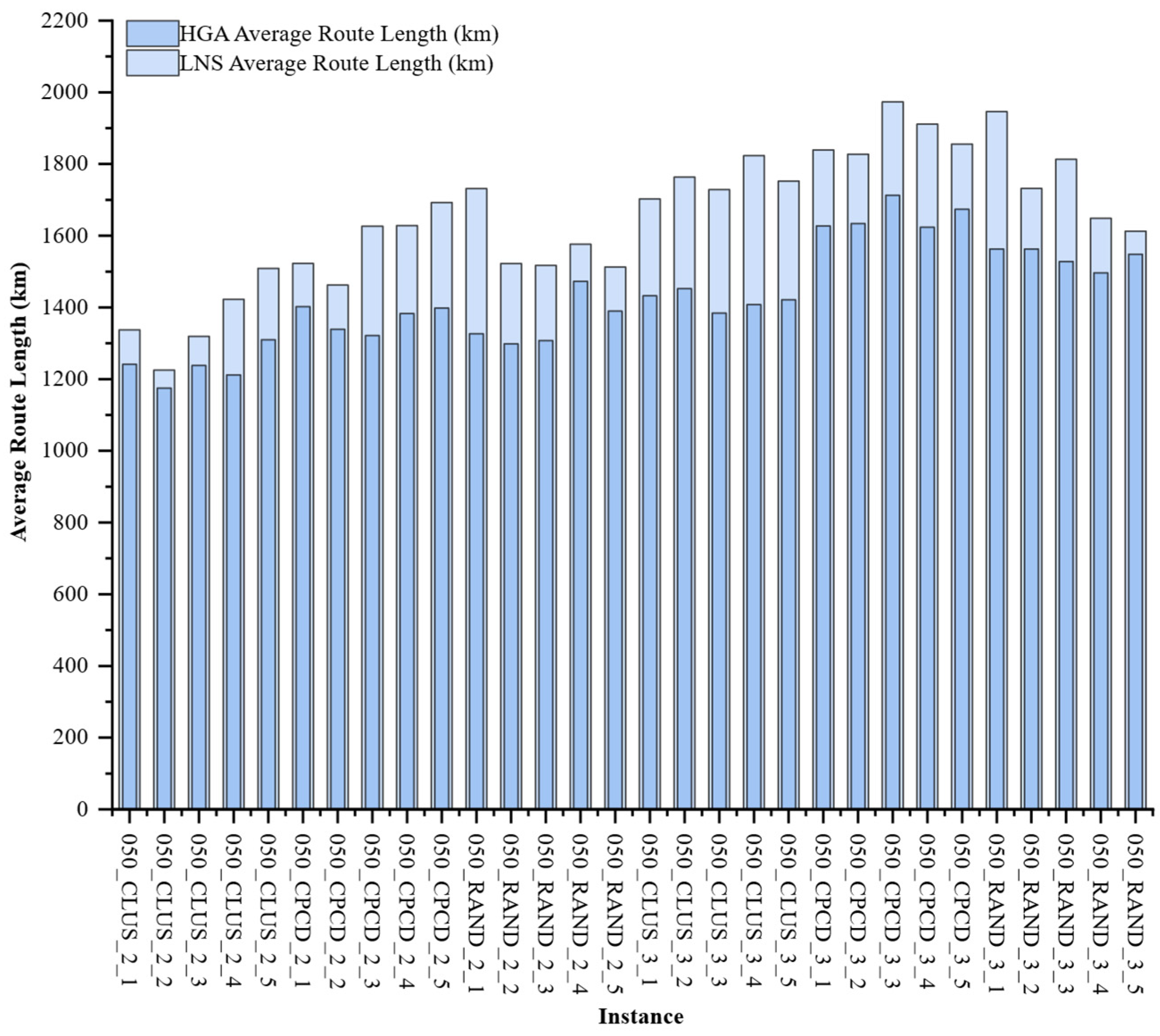
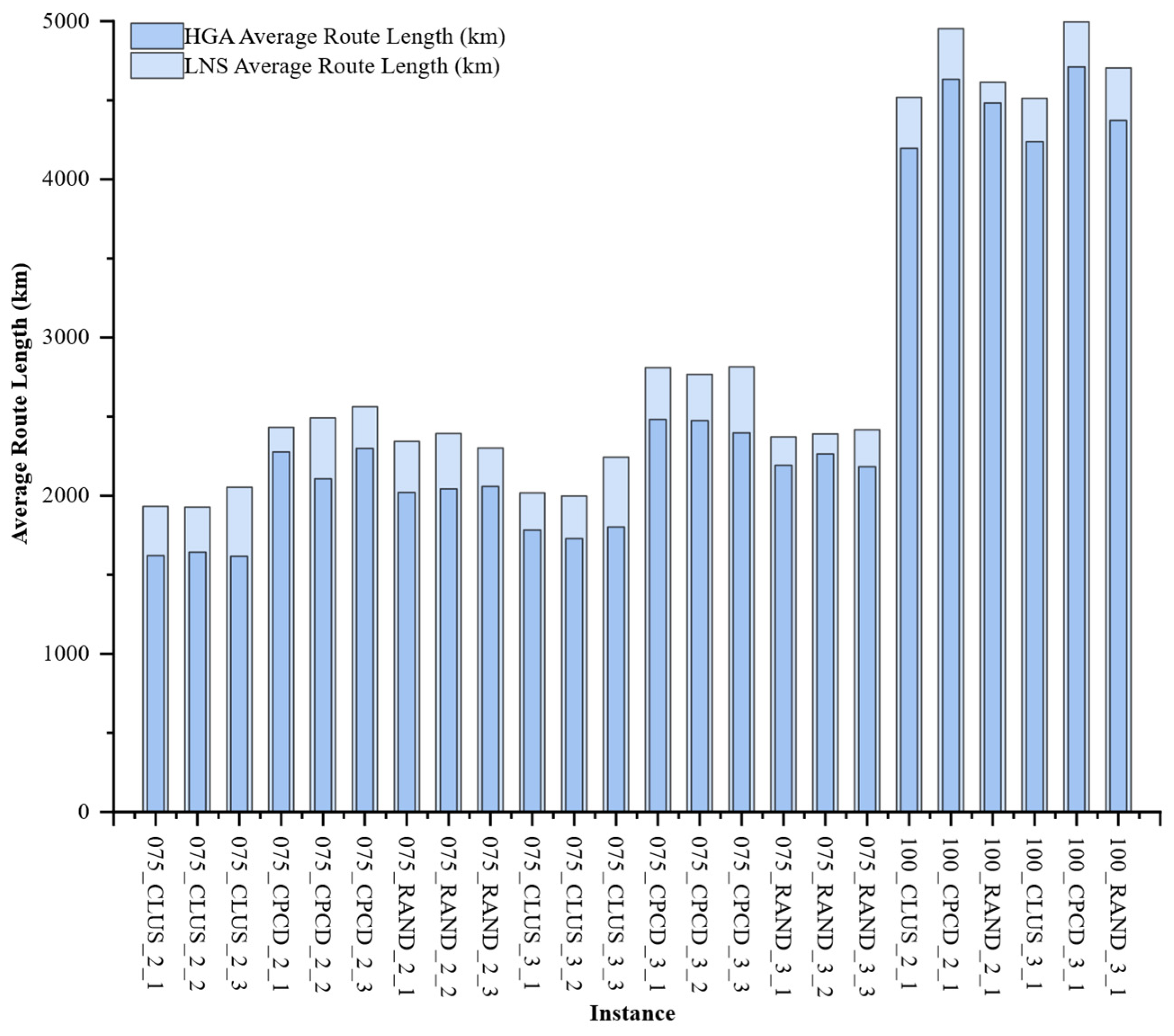
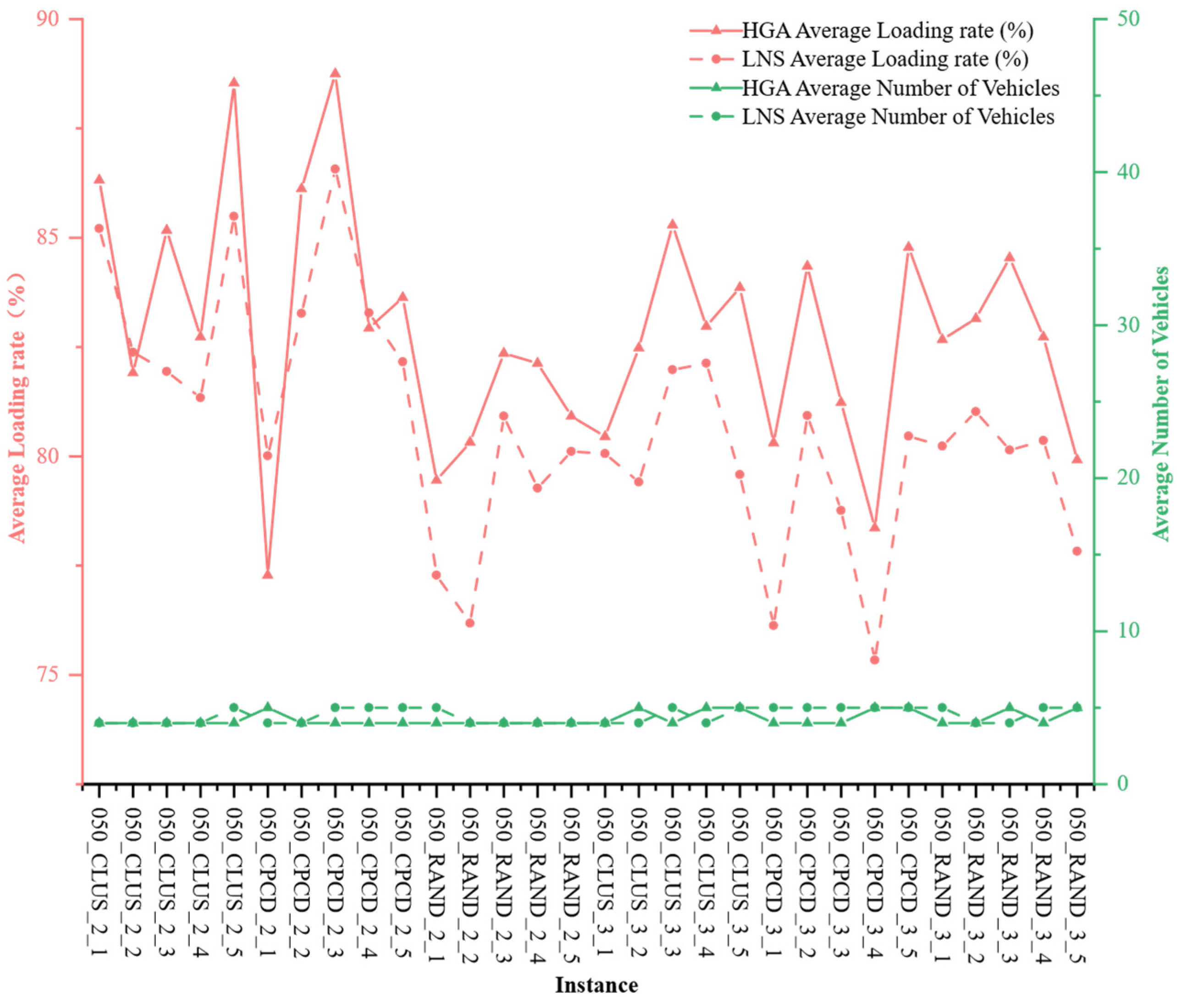
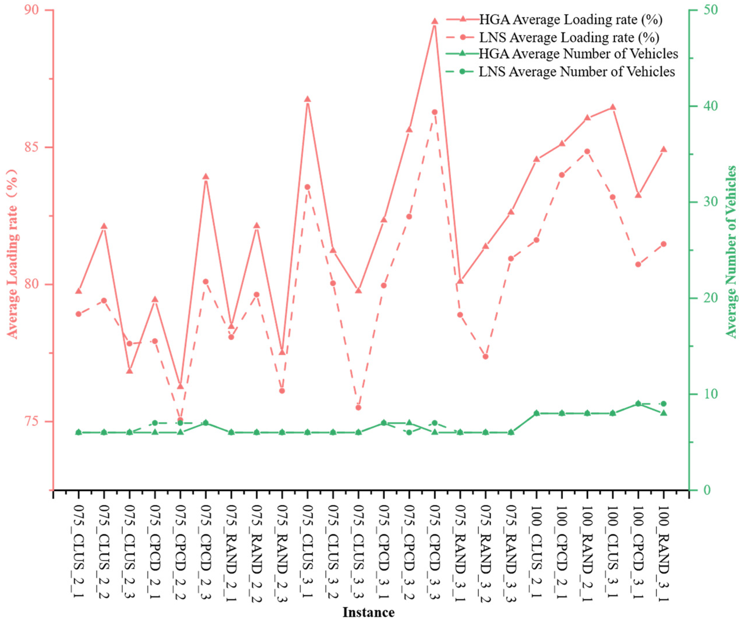
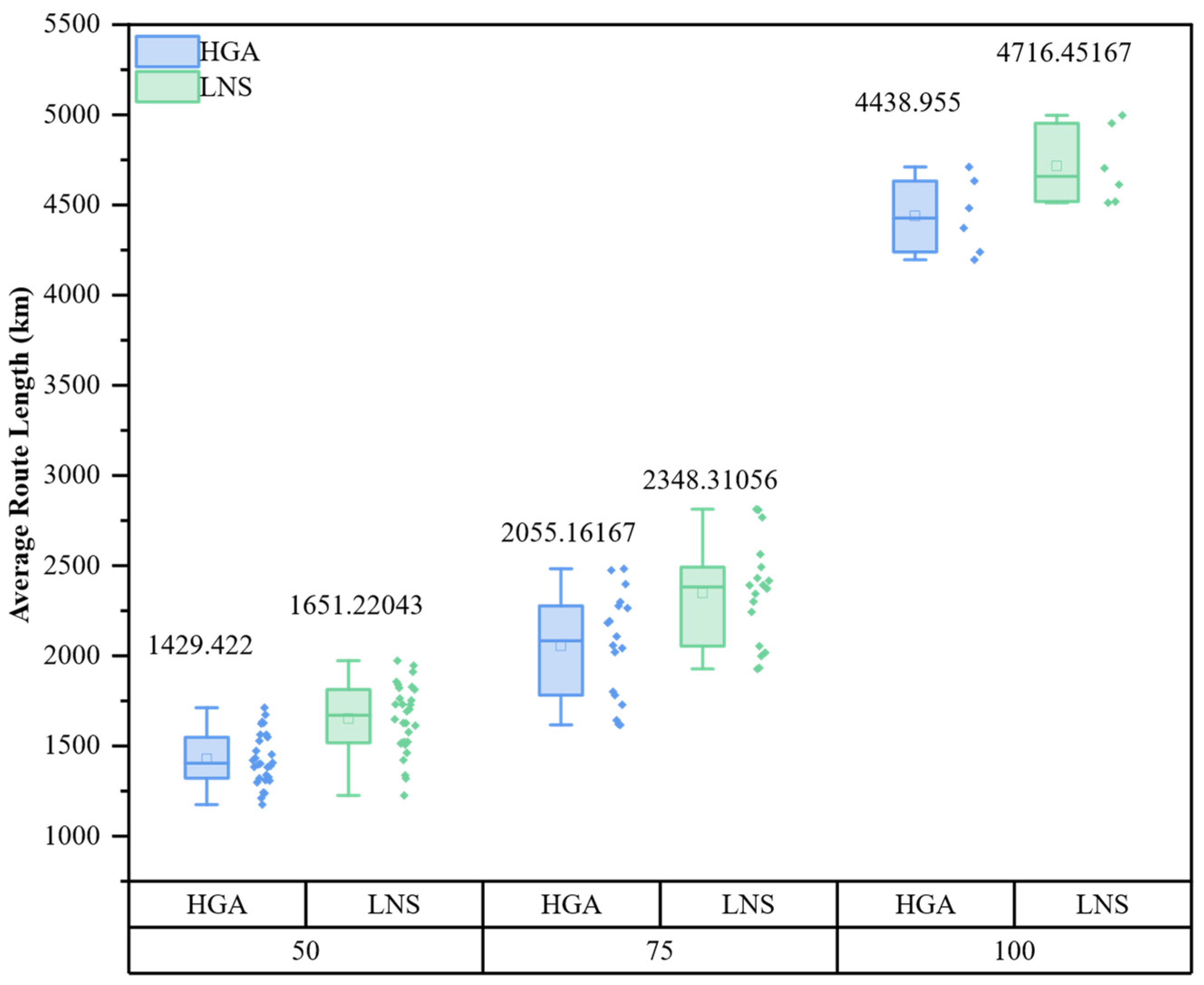
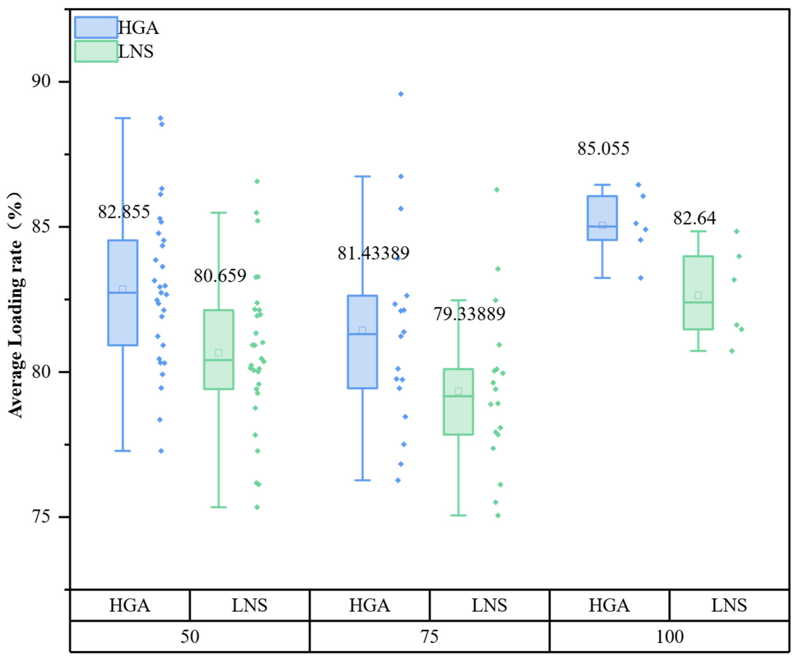
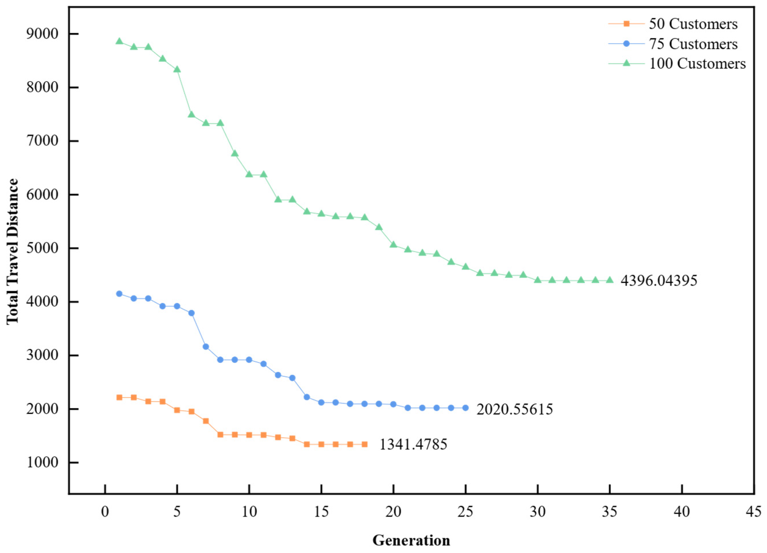
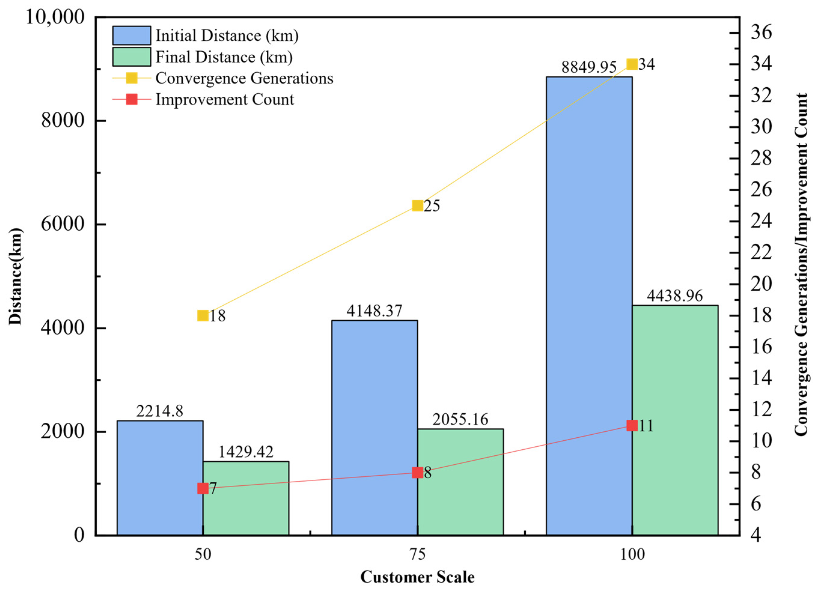
Computational experiments conducted on extended benchmark instances derived from standard 3L-PDP datasets demonstrate that the proposed algorithm can reliably generate feasible delivery plans that combine shorter vehicle routes with greater spatial utilization. Compared with an LNS-based baseline from the literature, the average vehicle travel distance is reduced by 10.60%, and the average loading rate is increased by 2.76%. Our analysis of convergence characteristics demonstrates that the algorithm maintains robustness and solution quality even as the customer scale increases from 50 to 100 nodes, effectively handling the trade-off between minimizing travel costs and maximizing vehicle fill rates under complex physical constraints. The HGA algorithm requires more CPU time than the LNS algorithm, primarily due to its group-based evolutionary algorithm characteristics and the iterative three-dimensional load verification process. This process significantly enhances the quality and feasibility of the solutions.

This study provides a practical solution framework for logistics distribution optimization under complex one-to-many 3L-PDVRP, offering practical value for reducing transportation costs and enhancing operational efficiency. However, real-world logistics scenarios possess greater dynamism and complexity; therefore, future research could further deepen the investigation into networked delivery modes involving multi-distribution center coordination.