Efficiency and Potential of China’s Aquatic Product Exports to Belt and Road Countries: Evidence from a Stochastic Frontier Gravity Model

Abstract

In the context of the sustainable transformation of the blue food system, aquatic product exports are shaped by trade scale, institutional conditions, and market access requirements. Using an unbalanced panel of China’s aquatic product exports to 39 countries along the Belt and Road from 2006 to 2023, this paper applies the BC95 one-step stochastic frontier gravity model to estimate trade efficiency and export potential. The results show that: (1) Significant trade inefficiency exists, with an average efficiency of 0.3696. (2) In the baseline model, China’s GDP, destination-country GDP and population, and common language are positively associated with exports, while geographical distance is negatively associated with exports. Political stability, government effectiveness, and trade freedom are associated with lower trade inefficiency, whereas destination-country aquatic product production and halal certification requirements are associated with higher trade inefficiency. Robustness tests broadly support the main findings, although the estimates for destination-country population, common language, and government effectiveness are more specification-sensitive. (3) A scale–efficiency matrix classifies 33 export markets into four sample-relative groups. The findings suggest that China’s aquatic product exports should shift from scale expansion toward a sustainable trade development model that places greater emphasis on efficiency, quality, compliance, and stability, with differentiated strategies across export markets.

1. Introduction

Blue foods are foods sourced from aquatic environments and encompass a diverse range of wild-caught and farmed aquatic species. The blue food system encompasses the actors and activities involved in the production, processing, distribution, trade, and consumption of these foods. Blue foods contribute to nutritional security, food-system sustainability, and the livelihoods of people who depend on aquatic value chains [1]. China is a major exporter of aquatic products globally and an important participant in international aquatic product trade [2]. The Belt and Road Initiative (BRI) is an international cooperation framework aimed at strengthening connectivity, and economic and trade cooperation across Asia, Europe, and Africa. For China, the BRI has become an important platform for advancing high-standard opening-up and deepening international economic and trade cooperation. The report to the 20th National Congress of the Communist Party of China called for promoting high-quality Belt and Road cooperation [3]. The 14th Five-Year Plan for National Fisheries Development also emphasized expanding aquatic product markets, advancing open development, and strengthening international fisheries cooperation [4]. Across the initial 64-country frame, China’s aquatic product exports increased from approximately USD 0.743 billion in 2006 to USD 5.285 billion in 2023. And their share of China’s total exports under the same product definition rose from 8.19% to 27.25%, indicating that these markets have become an important driver of China’s aquatic product export growth and market diversification. However, growth in export value does not necessarily translate into corresponding improvements in trade efficiency, stability, and sustainability. Aquatic products are perishable, highly sensitive to transportation time, and subject to stringent food-safety requirements. Their cross-border trade is therefore vulnerable to transport delays, logistics constraints, and stringent regulatory requirements. Transport and customs clearance delays can increase trade costs and adversely affect the quality, price, and export value of perishable products [5,6]. Food safety standards and related regulations may also raise firms’ compliance costs and affect their ability to maintain access to international markets [7,8]. External shocks may further affect China’s fish and crustacean product exports through transport disruptions, border controls, and shifts in demand [9]. Therefore, export value alone is insufficient for evaluating the performance and sustainability of China’s aquatic product trade. A fuller assessment requires evidence on the gap between observed export value and the estimated trade frontier, the factors associated with trade inefficiency, and the conditions under which model-implied export potential could be realized. In this study, sustainability is defined in economic and institutional terms: stable trade relationships, reduced institutional and logistics frictions, stronger compliance capabilities, and realistic conditions for realizing model-implied export potential.

Existing research on aquatic product trade has focused primarily on its determinants and regional variation. On the supply and demand sides, the production capacity of aquatic products, consumer demand, population size, and income level help explain international trade in aquatic products [10]. Changes in destination-market demand can also significantly affect fluctuations in China’s aquatic product exports [11]. Geographical distance and transportation costs affect the scale of cross-border aquatic product trade, while free trade agreements and regional cooperation arrangements may influence export performance by improving market access and trade facilitation [10,12,13]. Trade pattern also vary by product form, product category, and partner characteristics [2]. Free trade agreements, regional cooperation arrangements, and environmental provisions form part of the institutional setting for aquatic product trade, although their estimated associations vary across studies [12,14]. At the regional level, existing studies have covered global trade networks, RCEP member countries, and some national markets. The global fish and fish product trade network has become increasingly interconnected, although countries differ in their network positions and vulnerability to external shocks [15]. China’s aquatic product trade with RCEP members also exhibits both competition and complementarity [16]. Prior studies explain aquatic product trade in terms of supply and demand; trade costs; product heterogeneity; and institutional conditions across global, RCEP, and selected national settings. Systematic evidence remains limited, however, on the efficiency of China’s exports to RI partners, the correlates of trade inefficiency, and the conditions for realizing model-implied export potential.

The trade gravity theory posits that bilateral trade flows are closely related to the economic size of trading partners and are constrained by bilateral and multilateral trade costs [17,18]. Conventional gravity models are useful for explaining observed bilateral trade flows, but they do not distinguish random shocks from systematic departures of observed trade from the attainable trade frontier. Consequently, they cannot directly measure trade efficiency or separate unrealized trade potential from random variation. A stochastic frontier model decomposes the composite error into a symmetric random component and non-negative inefficiency component, thereby separating random shocks from estimated efficiency losses [19,20]. Embedded in a gravity framework, the model can estimate the gap between observed export values and the estimated trade frontier, and thereby derive trade efficiency and potential export values [21,22]. In recent years, the approach has increasingly been applied to agricultural trade. Studies of agricultural trade efficiency have considered economic size, distance, BRI cooperation, free trade agreements, market openness, and shipping connectivity, with coefficient signs and statistical significance varying across settings [21,23,24]. Cao et al. [25] found that institutional openness, tariffs, and customs-clearance conditions are associated with the efficiency of China’s agricultural imports from Central Asian countries. Shi et al. [22] reported that tariffs, liner shipping connectivity, government effectiveness, and monetary freedom were significantly associated with trade inefficiency in China’s agricultural exports to RCEP members. Stochastic frontier gravity models have been applied predominantly to the agricultural sector as a whole or to broad categories of agricultural products, with relatively limited applications to aquatic product trade.

In summary, although existing studies have examined aquatic product trade patterns and applied stochastic frontier gravity models to agricultural trade, limited attention has been paid to the gap between observed aquatic product exports and the estimated trade frontier, the factors associated with that gap, and cross-country differences in market performance. To address these gaps, this study adopts a trade-efficiency perspective and applies the Battese–Coelli [20] one-step stochastic frontier gravity model to data on China’s aquatic product exports from 2006 to 2023. The initial frame comprised 64 BRI partner countries, the preferred estimation sample retained 39 destinations for which the export outcome and all variables in the frontier and inefficiency equations were jointly observed. Because annual data coverage varies across destinations, an unbalanced panel allows broader country coverage while avoiding imputation of unreported observations. Accordingly, the study pursues four objectives: (1) to estimate the overall, annual, and destination-specific trade efficiency of China’s aquatic product exports to 39 BRI countries; (2) to identify the factors associated with the export frontier and trade inefficiency; (3) to estimate country-level export potential and the gaps between observed and frontier export values; and (4) to classify destination markets by export scale and trade efficiency, with export potential used as supplementary information.

This study makes four related contributions. First, it extends the trade-efficiency framework to the aquatic-products sector. Second, it distinguishes factors associated with the export frontier from factors associated with inefficiency in reaching that frontier. Third, it incorporates destination-country aquatic product production and halal certification requirements into the inefficiency equation. Finally, it translates the estimated efficiency and export scale into a country-level market classification and evaluates the classification’s sensitivity to alternative cutoff rules.

The remainder of the paper is organized as follows. Section 2 describes the development and structure of China’s aquatic product exports to countries along the Belt and Road. Section 3 presents the theoretical framework, model specification, and data. Section 4 reports the model tests and estimation results. Section 5 examines trade efficiency, export potential, and market classification. Section 6 presents robustness and sensitivity analyses. Section 7 concludes and provides policy implications.

2. Descriptive Overview of China’s Aquatic Product Exports to the 39 Countries Along the Belt and Road Initiative

2.1. Export Scale

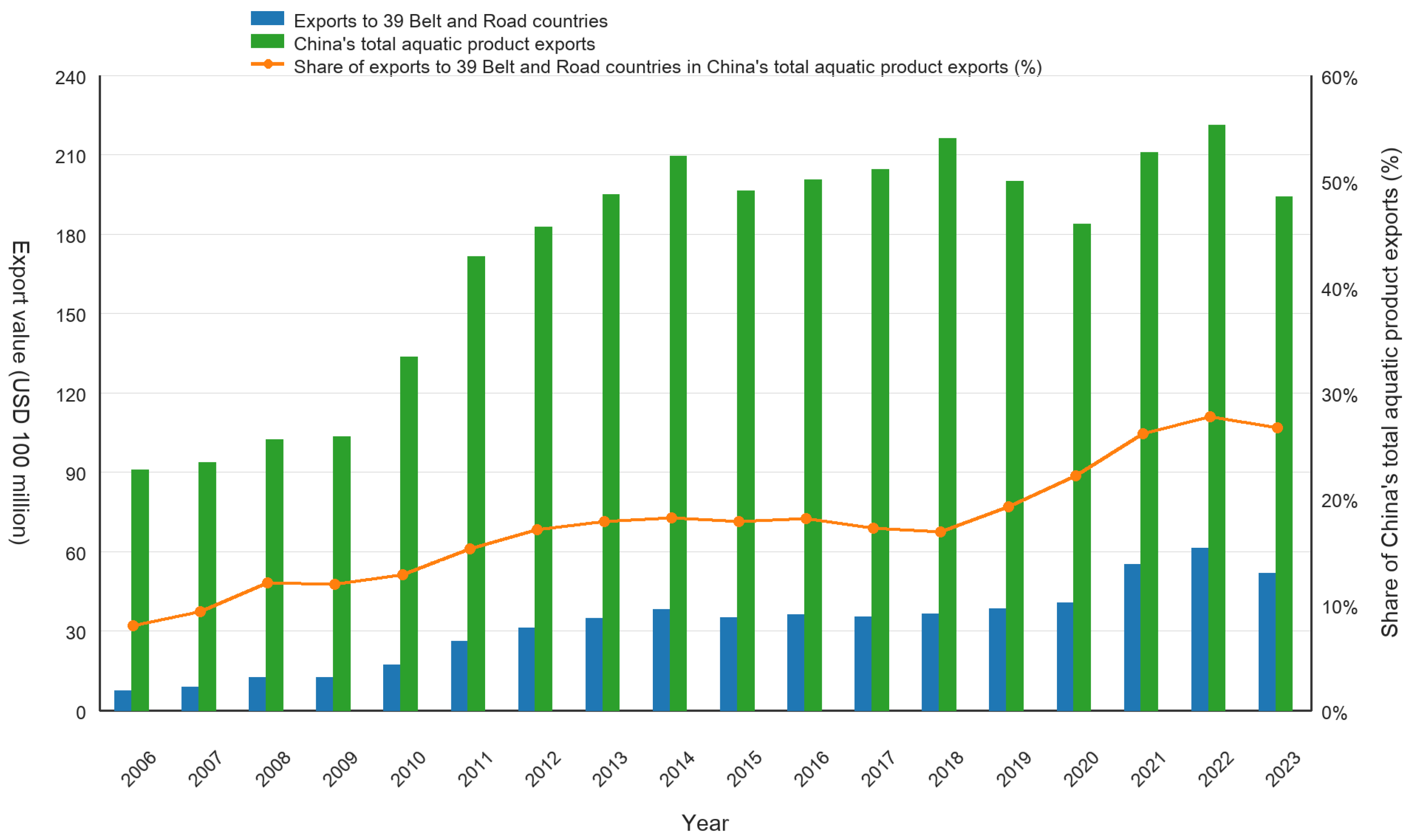
As shown in Figure 1, the value of China’s aquatic product exports to the 39 sample countries increased overall between 2006 and 2023, despite year-to-year fluctuations. The export value rose from USD 726 million in 2006 to USD 5.180 billion in 2023, reaching approximately 7.13 times its initial level, with an average annual growth rate of about 12.25%. Over the same period, the share of these 39 countries in China’s total aquatic product exports rose from 8.00% to 26.71%, an increase of 18.71 percentage points. These figures indicate that the 39 markets have accounted for an increasing share of China’s aquatic product exports over the study period.

From 2006 to 2014, China’s aquatic product exports to the 39 Belt and Road countries expanded rapidly, rising from USD 726 million to USD 3.799 billion. Between 2015 and 2019, export value fluctuated within a relatively narrow range, from USD 3.495 billion to USD 3.848 billion. Exports increased further after 2020, reaching USD 5.508 billion in 2021 and peaking at USD 6.130 billion in 2022, before declining to USD 5.180 billion in 2023. The export share followed a broadly similar upward pattern, reaching its highest level of 27.71% in 2022 and remaining at 26.71% in 2023. Although both export value and market share increased substantially, expansion in export scale alone does not necessarily imply higher trade efficiency or greater sustainability. Trade efficiency, sources of inefficiency, and export potential therefore require further examination.

2.2. Export Product Composition

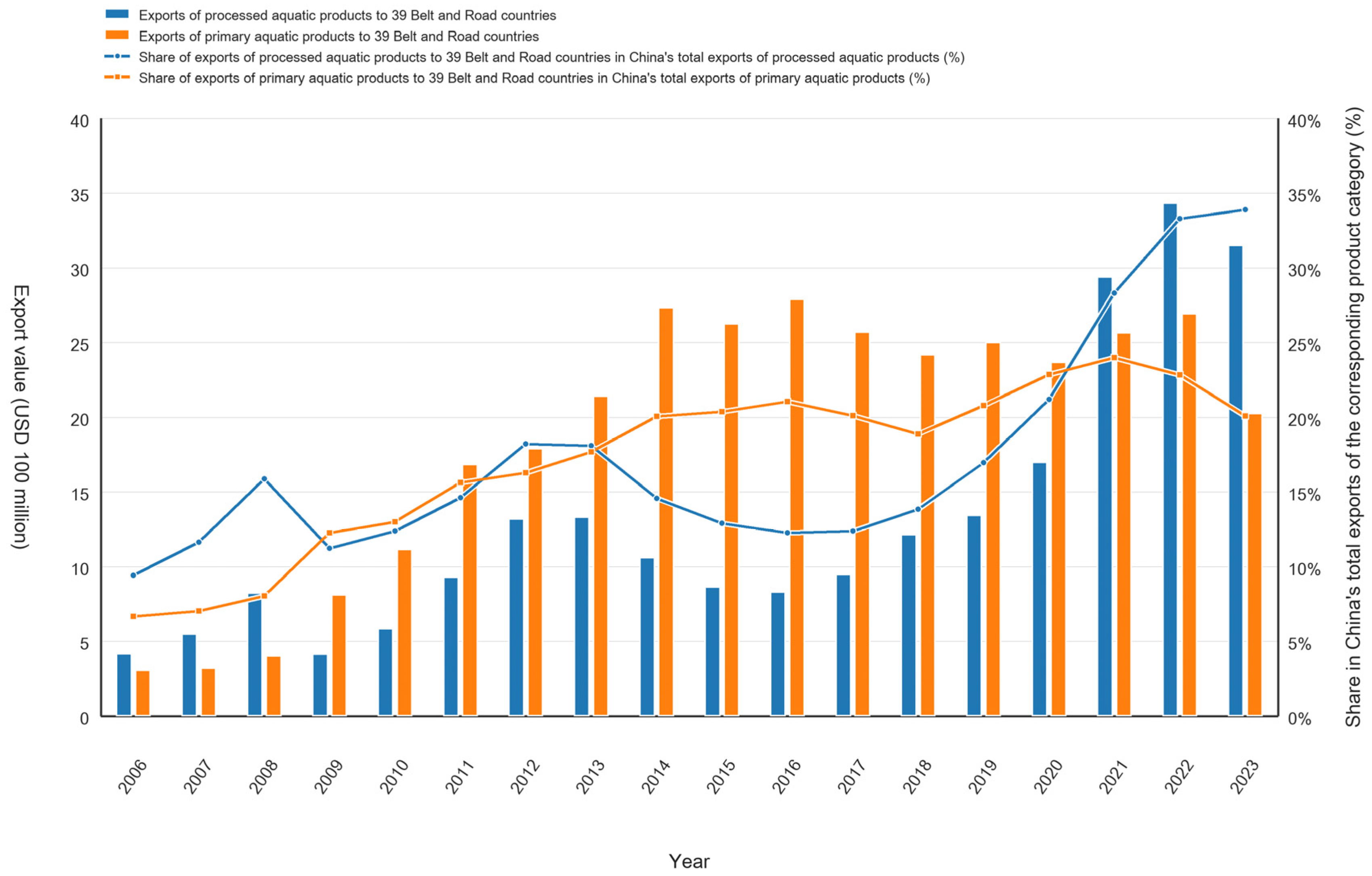
Following Liu and Yang [16], this study classifies HS03019 (all six-digit codes beginning with 03019), HS0302-0304, HS0306-0308, and HS12122 (all six-digit codes beginning with 12122) as primary aquatic products, and HS0305, HS0309, HS1604, and HS1605 as processed aquatic products. Figure 2 shows that, between 2006 and 2023, the export value of processed aquatic products from China to the 39 sample countries increased from USD 0.417 billion to USD 3.154 billion, while the export value of primary aquatic products rose from USD 0.309 billion to USD 2.027 billion. Both product categories showed an overall upward trend, although their relative export shares changed across different periods.

From the perspective of product structure, China’s aquatic product exports to the 39 sample countries showed a clear phased pattern. From 2006 to 2008, the export value of processed aquatic products was higher than that of primary aquatic products; from 2009 to 2020, primary aquatic products became the larger category; and from 2021 onward, processed aquatic products again recorded the higher export value. During the same period, the share of processed aquatic product exports to these 39 countries in China’s total exports of processed aquatic products increased from 9.40% in 2006 to 33.90% in 2023. The corresponding share for primary aquatic products rose from 6.66% to 20.08%, reaching a peak of 23.99% in 2021 before declining in the following two years. Since 2021, the export value of processed aquatic products to these countries has exceeded that of primary aquatic products.

2.3. Destination-Market Distribution

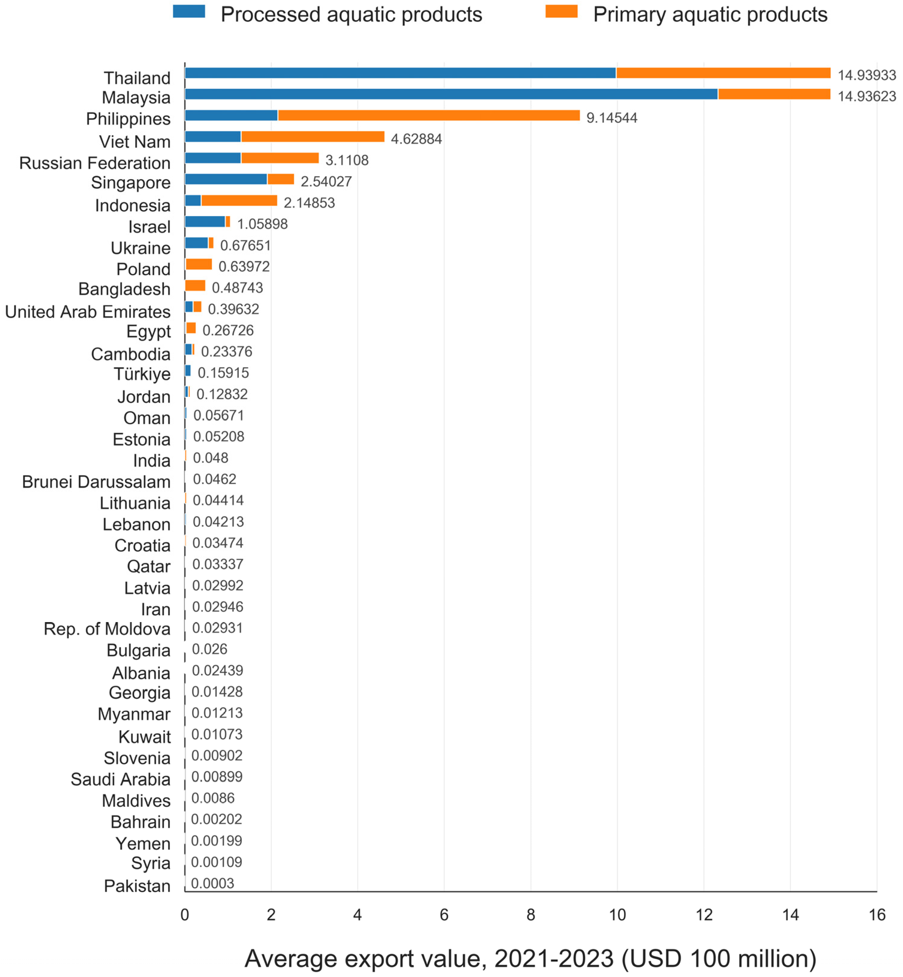
As shown in Figure 3, China’s aquatic product exports to the 39 countries along the Belt and Road are relatively concentrated in a small number of markets. Based on the average export value from 2021 to 2023, Thailand and Malaysia are the two largest markets for China’s aquatic product exports to these countries, while the Philippines ranks third. Countries such as Vietnam, Russia, Singapore, and Indonesia also have considerable export values. These patterns identify Southeast Asia and selected Eurasian destinations as the principal markets within the 39-country sample.

Export patterns also vary by product type. Processed aquatic product exports are concentrated in Malaysia, Thailand, the Philippines, Singapore, Vietnam and Russia, whereas primary aquatic product exports are concentrated in the Philippines, Thailand, Vietnam, Malaysia, Russia and Indonesia. The composition of China’s aquatic product exports therefore varies across destination markets, indicating heterogeneity in both product types and destination markets within the 39 BRI sample countries.

3. Methodology

3.1. Theoretical Modeling

3.1.1. Stochastic Frontier Gravity Model

The stochastic frontier model was first introduced by Aigner et al. [19], and it is mainly used to estimate the technical efficiency issues in production functions. The model decomposes the composite error term into a symmetric random-noise component and a non-negative inefficiency component. Adapting the stochastic frontier framework to bilateral export value, the trade model is specified as follows (Equation (1)):

$$Y_{ijt}= f\left({\mathit{X}}_{ijt},\mathit{\beta }\right)\mathrm{e}\mathrm{x}\mathrm{p}\left({\nu }_{ijt}\right)\mathrm{e}\mathrm{x}\mathrm{p}\left(-{\mu }_{ijt}\right),{ \mu }_{ijt}\ge 0$$

(1)

Taking the natural logarithm of Equation (1), we obtain:

$$\ln Y_{ijt}=\ln f\left({\mathit{X}}_{ijt},\mathit{\beta }\right)+{\nu }_{ijt}-{\mu }_{ijt},{ \mu }_{ijt}\ge 0$$

(2)

$Y_{ijt}$ represents observed bilateral export value from country i to country j in year t, ${\mathit{X}}_{ijt}$ is the vector of frontier covariates, and $\mathit{\beta }$ is the corresponding parameter vector. ${\nu }_{ijt}$ is a symmetric random error term, conventionally assumed to follow a zero-mean normal distribution and capture measurement error and other random shocks. ${\mu }_{ijt}$ is a non-negative inefficiency term, which is generally assumed to be independent of ${\nu }_{ijt}$ and to follow a half-normal distribution or a truncated normal distribution. When ${\mu }_{ijt}=0$, the observation lies on the stochastic export frontier, implying full trade efficiency:

$${Y_{ijt}}^{\mathit{*}}=f\left({\mathit{X}}_{ijt},\mathit{\beta }\right)\mathrm{e}\mathrm{x}\mathrm{p}\left({\nu }_{ijt}\right)$$

(3)

${Y_{ijt}}^{*}$ denotes the observation-specific model-implied frontier export value and can be interpreted as potential exports under the model assumptions. In this framework, the frontier value refers to the export value implied by the estimated stochastic frontier, rather than the conditional mean produced by a conventional gravity model.

Trade efficiency is defined as the ratio of observed export value to the model-implied frontier value:

$${TE}_{ijt}=Y_{ijt}/{Y_{ijt}}^{\mathit{*}}=\mathrm{e}\mathrm{x}\mathrm{p}\left(-{\mu }_{ijt}\right),{\mu }_{ijt}\ge 0$$

(4)

${TE}_{ijt}\in \left(\mathrm{0,1}\right]$. The closer the trade efficiency is to 1, the more the observed export value is close to the potential export frontier, and the lower the trade inefficiency is. And, values closer to 0 indicate a larger relative gap between observed exports and the estimated frontier.

When the time dimension of the data in the model is relatively long, the original assumption of constant technical efficiency may fail to reflect the actual situation where efficiency changes over time. To address this issue, Battese and Coelli [26] further proposed a time-varying stochastic frontier model, setting the inefficiency term ${\mu }_{ijt}$ in a time-varying form:

$${\mu }_{ijt}=\left\{\mathrm{e}\mathrm{x}\mathrm{p}\left[-\eta \left(t-T\right)\right]\right\}{\mu }_{ij}$$

(5)

${\mu }_{ijt}$ represents the level of trade inefficiency, $\eta$ is the parameter to be estimated, and T represents the last year of the sample period. When $\eta >0$, it indicates that the trade inefficiency term gradually decreases over time. When $\eta =0$, it means that the trade inefficiency term does not change over time. When $\eta <0$, it indicates that the trade inefficiency term gradually increases over time.

3.1.2. Trade Inefficiency Model

Although the stochastic frontier gravity model separates trade inefficiency from random noise, explaining systematic variation in trade inefficiency requires an inefficiency-effects equation that relates inefficiency to observed explanatory factors. Earlier studies mostly adopted a two-step procedure: they estimated efficiency and then regressed the estimates on proposed explanatory variables. The first step typically assumes independently and identically distributed inefficiency, whereas the second explains variation in the same term using exogenous variables, and the assumptions imposed in the two steps may therefore be inconsistent. The second step may also ignore estimation error in the generated efficiency measure. Battese and Coelli [20] proposed a one-step inefficiency-effects model that jointly estimates the stochastic frontier and the conditional mean of trade inefficiency, thereby allowing the determinants of inefficiency to be incorporated directly into the frontier estimation. In the one-step method analysis, the trade inefficiency term is:

$${\mu }_{ijt}=\mathit{\lambda }{\mathit{K}}_{ijt}+{\omega }_{ijt}$$

(6)

$\mathit{\lambda }$ denotes the vector of parameters to be estimated, ${\mathit{K}}_{ijt}$ denotes the vector of observed covariates associated with trade inefficiency, and ${\omega }_{ijt}$ denotes the truncated-normal disturbance term. By combining Equations (2) and (6), the modified stochastic frontier gravity model can be further obtained as follows:

$$\ln Y_{ijt}=\ln f\left({\mathit{X}}_{ijt},\mathit{\beta }\right)+{\nu }_{ijt}-\left(\mathit{\lambda }{\mathit{K}}_{ijt}+{\omega }_{ijt}\right)$$

(7)

Thus, the one-step framework jointly estimates the export-frontier and inefficiency-effects equations, thereby avoiding distributional inconsistency of the two-step procedure and accounting for uncertainty in the inefficiency term.

3.2. Model Specification

3.2.1. Stochastic Frontier Trade Equation

With China as the exporter and the 39 sample countries along the Belt and Road as the destination, the stochastic export-frontier equation is specified as follows (Equation (8)):

$$\begin{array}{c}\ln Y_{ijt}={\beta }_0+{\beta }_1\ln {GDP}_{it}+{\beta }_2\ln {GDP}_{jt}+{\beta }_3\ln {POP}_{jt}\\ +{\beta }_4\ln {Dist}_{ij}+{\beta }_5{Comlang}_{ij}{+\nu }_{ijt}-{\mu }_{ijt}\end{array}$$

(8)

where $i$ represents China and $j$ represents the destination country. $Y_{ijt}$ represents the value of China’s aquatic product exports to destination $j$ in year $t$. ${GDP}_{it}$ and ${GDP}_{jt}$, respectively, represent the gross domestic product of China and destination $j$. ${POP}_{jt}$ represents the population size of the destination country. ${Dist}_{ij}$ represents the geographical distance between China and the destination country. ${Comlang}_{ij}$ represents whether China and the destination country share a common language. ${\nu }_{ijt}$ is the random error term. ${\mu }_{ijt}$ is a non-negative trade inefficiency term.

3.2.2. Trade Inefficiency Equation

The inefficiency-effects equation includes free trade agreements, political stability, government effectiveness, monetary freedom, trade freedom, financial freedom, and the liner shipping connectivity index. Destination-country aquatic production and halal certification requirements are included to capture industry-specific market conditions. The equation is specified as follows (Equation (9)):

$$\begin{array}{c}{\mu }_{ijt}={\delta }_0+{{\delta }_{1}FTA}_{ijt}+{{\delta }_{2}PS}_{jt}+{{\delta }_{3}GE}_{jt}+{\delta }_4\ln {MF}_{jt}+{\delta }_5\ln {TF}_{jt}\\ +{\delta }_6\ln {FF}_{jt}+{\delta }_7\ln {LSCI}_{jt}+{\delta }_8\ln {PROD}_{jt}+{\delta }_9{HALAL}_j+{\omega }_{ijt}\end{array}$$

(9)

${FTA}_{ijt}$ indicates whether a formal free trade agreement between China and the destination country has been officially implemented. ${PS}_{jt}$ represents the political stability of the destination country. ${GE}_{jt}$ represents the government effectiveness of the destination country. ${MF}_{jt}$, ${TF}_{jt}$, and ${FF}_{jt}$, respectively, represent destination-country monetary freedom, trade freedom, and financial freedom. ${LSCI}_{jt}$ represents the liner shipping connectivity index of destination country $j$ in year $t$. ${PROD}_{jt}$ denotes total aquatic production in destination $j$ in year $t$, while ${HALAL}_j$ indicates whether relatively stringent halal certification requirements apply in the destination market. ${\omega }_{ijt}$ is a random disturbance term.

3.3. Data Sources and Processing

This study uses annual data on China’s aquatic product exports to Belt and Road countries from 2006 to 2023. The initial country frame comprises 64 BRI partner countries (listed in Table S1 of Supplementary Materials), yielding 1152 potential country-year observations. Of these, 1019 observations from 63 countries contain recorded positive export values. Export values are unavailable for 133 country-year combinations, and the source contains no explicitly recorded zero export values. After requiring complete data for the core gravity variables, 938 observations from 58 countries remain. Requiring valid observations for every variable in the preferred one-step specification further reduces the sample to 648 observations from 39 countries. These observations constitute the unbalanced panel used in the main analysis. Of the 39 destination countries, 26 have complete observations for all 18 years, yielding 468 observations; this balanced subsample is used to assess sensitivity to panel structure.

Since the temporal patterns surrounding these gaps did not provide a defensible basis for treating them as zero or assuming linear changes between adjacent years, no missing value was interpolated or replaced with zero. Continuous variables specified in logarithmic form were retained only when strictly positive recorded values were available, whereas zero values of binary indicators were retained according to their substantive definitions. Observations lacking any variable required by the preferred specification were excluded at the country-year level. A variable-level audit of missing and non-positive observations is reported in Table S2 of the Supplementary Materials.

The statistical scope of aquatic products follows Liu and Yang [16] and is aligned with the HS codes observed for the sample countries during 2006–2023.

Table 1. Categories of aquatic products under the HS classification standards.

HS Code Range	Category Name
03019 *	Other live fish
0302	Fresh and chilled fish, except for fish fillets and other fish meat with tax code 03.04
0303	Frozen fish, except for fish fillets and other fish meat with tax code 03.04
0304	Fresh, chilled, and frozen fish fillets and other fish meat, whether minced or not
0305	Pickled and smoked fish, and fish meal for human consumption
0306	Crustaceans with shells or shells removed
0307	Mollusks with shells or shells removed
0308	Aquatic invertebrates that are not crustaceans or mollusks
0309	Fine powder; coarse powder; and granules of fish, crustaceans, mollusks, and other aquatic invertebrates suitable for human consumption
12122 *	Seaweed and other algae
1604	Fish that has been prepared or preserved; sturgeon caviar and substitutes for sturgeon caviar made from fish eggs
1605	Prepared or preserved crustaceans, mollusks, and other aquatic invertebrates

Note: * indicates an aggregated HS-code range comprising all six-digit codes beginning with the listed five-digit prefix; it does not denote a single six-digit HS code. Accordingly, HS03019 represents other live fish-related codes starting with HS03019, and HS12122 represents the codes for seaweeds and other algae starting with HS12122.

reports the HS-code coverage used to define aquatic products.

Data from different sources were merged by country code and year, with currency units, measurement units, and variable names standardized before estimation. Export value, GDP, population, geographical distance, liner shipping connectivity, aquatic production, monetary freedom, trade freedom, and financial freedom were transformed using natural logarithms. The transformations reduce skewness and provide a scale based on proportional rather than absolute changes, facilitating the interpretation of coefficients in the log-linear specification. Free trade agreements, common language, and halal certification requirements were coded as binary indicators. Observations with missing values required for the full model specification are excluded from the corresponding estimation sample, and no interpolation is applied. The resulting main sample consists of an unbalanced panel of 39 countries along the Belt and Road from 2006 to 2023. Variable definitions, data sources, and expected coefficient signs are reported in

Table 2. Variable description and expected coefficient signs.

Variable	Definition	Data Source	Expected Sign
Frontier Equation Variables
$Y_{ijt}$	Value of China’s aquatic product exports	UN Comtrade Database	/
${GDP}_{it}$	China’s gross domestic product	World Development Indicators, World Bank	+
${GDP}_{jt}$	Destination country’s gross domestic product	World Development Indicators, World Bank	+
${POP}_{jt}$	Population of the destination country	World Development Indicators, World Bank	+
${Dist}_{ij}$	Geographical distance	CEPII Database	−
${Comlang}_{ij}$	Whether China and the destination country share a common official language	CEPII Database	+
Trade Inefficiency Equation Variables
${FTA}_{ijt}$	Whether a free trade agreement is in force	China FTA Network	−
${PS}_{jt}$	Political stability of the destination country	Worldwide Governance Indicators, World Bank	−
${GE}_{jt}$	Government effectiveness of the destination country	Worldwide Governance Indicators, World Bank	−
${MF}_{jt}$	Monetary freedom of the destination country	Index of Economic Freedom, The Heritage Foundation	−
${TF}_{jt}$	Trade freedom of the destination country	Index of Economic Freedom, The Heritage Foundation	−
${FF}_{jt}$	Financial freedom of the destination country	Index of Economic Freedom, The Heritage Foundation	−
${LSCI}_{jt}$	Liner Shipping Connectivity Index of the destination country	United Nations Conference on Trade and Development	−
${PROD}_{jt}$	Total fisheries production of destination country	World Development Indicators, World Bank	+
${HALAL}_j$	Whether relatively stringent halal certification requirements apply in the destination market	National regulations and materials from officially recognized halal certification bodies	+

Note: / indicates that no expected sign is specified for the dependent variable. In the frontier equation, + and − denote expected positive and negative associations, respectively, with the frontier export value; in the trade inefficiency equation, they denote expected positive and negative associations, respectively, with trade inefficiency.

. In the frontier equation, + and − indicate higher and lower frontier export values, respectively; in the inefficiency equation, + and −, respectively, represent higher and lower trade inefficiency. All model estimations and statistical tests were conducted using Stata/MP 18.0.

4. Results and Discussion

4.1. Model Applicability Test

Table 3. Likelihood-ratio tests for model specification and temporal structure.

Panel and Null Hypothesis	LL(R)	LL(U)	LR Statistic	Reference Distribution	p-Value	Decision
Panel A. Core model-selection tests
H01: No inefficiency effects,($\gamma ={\delta }_0=\cdots ={\delta }_9=0$)	−1369.316	−1138.623	461.385	Kodde–Palm bounds $(q=11)$	—	Reject at 1%
H02: The inefficiency component is non-stochastic, ($\gamma =0$)	−1258.792	−1138.623	240.339	Kodde–Palm bounds $(q=2)$	—	Reject at 1%
H03: All BC95 conditional-mean parameters are zero, (${\delta }_0=\cdots ={\delta }_9=0$)	−1280.680	−1138.623	284.115	${\chi }^2\left(10\right)$	<0.001	Reject
Panel B. Selection of the preferred BC95 specification
H04: ${\delta }_{PROD}={\delta }_{HALAL}=0$	−1162.739	−1138.623	48.232	${\chi }^2\left(2\right)$	<0.001	Reject
H05: Coefficients of $PS, GE, MF, TF, FF, LSCI$, and $PROD$ are jointly zero	−1213.120	−1138.623	148.994	${\chi }^2\left(7\right)$	<0.001	Reject

Note: The estimations use the same 39-country unbalanced panel comprising 648 observations over 2006–2023. $LL\left(\mathrm{R}\right)$ and $LL\left(\mathrm{U}\right)$ denote the maximized log-likelihoods of the restricted and unrestricted models, respectively. The unrestricted model for all tests is the full BC95 specification. The $LR$ statistic is calculated as $LR=-2\left[LL\left(\mathrm{R}\right)-lnLL\left(\mathrm{U}\right)\right]$. Because H01 and H02 involve parameters on the boundary of the parameter space and parameters that are not identified under the null, their $LR$ statistics are evaluated using the Kodde–Palm bounds rather than a conventional chi-square distribution. The reference distributions for H03, H04, and H05 are ${\chi }^2\left(10\right)$, ${\chi }^2\left(2\right)$, and ${\chi }^2\left(7\right)$, respectively. Source: Authors’ estimations based on the study dataset. Software: The models and statistical tests were estimated by the authors using Stata/MP 18.0.

reports the model specification tests based on the unbalanced panel of 39 countries. First, the joint null hypothesis of no inefficiency effects is rejected at the 1% level, indicating that the normal gravity model cannot adequately capture trade inefficiency in the sample. To further determine whether the improvement in model fit is due solely to the addition of the variables ${\mathit{K}}_{ijt}$, the variables from the stochastic frontier equation (${\mathit{X}}_{ijt}$) and the trade inefficiency equation (${\mathit{K}}_{ijt}$) are jointly included in a normal mean-response equation, and the stochastic nature of the inefficiency component is tested again. The null hypothesis of $\gamma =0$ is still rejected, indicating that the stochastic inefficiency component remains statistically significant even after controlling for these observable factors. On this basis, the full BC95 model provides a significantly better fit than the half-normal stochastic frontier model, as the joint restriction that all BC95 conditional-mean parameters are zero is rejected (LR = 284.115, p < 0.001). These tests indicate that trade inefficiency is not only stochastic but that its conditional mean is also systematically related to observed institutional, trade, logistics, and industry-specific characteristics, providing statistical support for the BC95 one-step inefficiency-effects model. The joint null hypothesis that the coefficients of $PROD$ and $HALAL$ are zero is also rejected (LR = 48.232, p < 0.001), supporting their joint inclusion in the final specification. The joint restriction on the remaining institutional, trade, logistics, and production variables is likewise rejected (LR = 148.994, p < 0.001), further supporting the full BC95 specification.

4.2. BC95 One-Step Estimates

Based on the model specification tests in Section 4.1, the full BC95 one-step specification is adopted as the preferred model.

Table 4. Estimation results of the BC95 one-step stochastic frontier gravity model.

Stochastic Frontier Equation			Trade Inefficiency Equation
Variable	Coefficient	z-Statistic	Variable	Coefficient	z-Statistic
$\ln {\mathrm{G}\mathrm{D}\mathrm{P}}_{\mathrm{i}\mathrm{t}}$	0.4598 ***	5.2416	${FTA}_{ijt}$	−0.8086	−0.8536
$\ln {\mathrm{G}\mathrm{D}\mathrm{P}}_{\mathrm{j}\mathrm{t}}$	0.6345 ***	9.5580	${PS}_{jt}$	−2.8983 ***	−3.7406
$\ln {POP}_{jt}$	0.5666 ***	8.7776	${GE}_{jt}$	−2.5978 **	−2.2214
$\ln {Dist}_{ij}$	−1.5842 ***	−8.5612	$\ln {MF}_{jt}$	5.4639	1.3876
${Comlang}_{ij}$	1.5922 ***	8.9854	$\ln {TF}_{jt}$	−7.7996 ***	−2.9853
$\mathrm{c}\mathrm{o}\mathrm{n}\mathrm{s}$.	−8.0167 **	−2.2992	$\ln {FF}_{jt}$	−0.2961	−0.2767
			$\ln {LSCI}_{jt}$	−0.6489	−1.0556
			$\ln {PROD}_{jt}$	1.0134 ***	3.4832
			${HALAL}_j$	5.1442 ***	4.4470
			$\mathrm{c}\mathrm{o}\mathrm{n}\mathrm{s}.$	−7.2660	−0.3766
${\sigma }^2$	14.8011 ***	4.8348	$\gamma$	0.9781 ***	161.8255
Log likelihood	−1138.623
$LR$ statistic	461.385
Observations	648
Mean trade efficiency	0.3696

Note: **, *** indicate significance at the 5%, and 1% significance levels, respectively. Source: Authors’ estimations based on the study dataset. Software: The models and statistical tests were estimated by the authors using Stata/MP 18.0.

reports the estimation results using the unbalanced panel of 39 countries along the Belt and Road. The estimates from this specification are used to calculate trade efficiency and export potential and to conduct the subsequent market classification analysis.

As a diagnostic check prior to estimation of the preferred BC95 one-step model, multicollinearity was assessed using Variance inflation factors (VIFs), calculated separately for the covariates in the stochastic frontier and inefficiency-effects equations using the same 39-country unbalanced estimation sample. The maximum VIFs were 3.73 for the frontier equation and 3.75 for the inefficiency equation, while the corresponding means were 2.11 and 2.14, respectively. All VIFs were below the conventional threshold of 10, suggesting that there was no multicollinearity problem in the preferred model. The detailed results are reported in Table S3 of the Supplementary Materials.

4.2.1. Results of the Frontier Equation

The estimation results of the frontier equation are presented in Table 4, the coefficients of China’s GDP ($\mathit{ln}{GDP}_{it}$), the GDP of the destination country ($\ln {GDP}_{jt}$), the population size of the destination country ($\ln {POP}_{jt}$), and the common language (${Comlang}_{ij}$) are all significantly positive. Holding other covariates constant, a 1% increase in China’s GDP, destination-country GDP, and destination-country population is associated with approximately 0.4598%, 0.6345%, and 0.5666% higher estimated export-frontier values, respectively. These findings are consistent with the expected roles of supply capacity, market size, and demand conditions in shaping the export frontier. The coefficient of geographical distance ($\ln {Dist}_{ij}$) is negative and statistically significant, suggesting that 1% greater geographical distance is associated with an approximately 1.5842% lower estimated frontier, consistent with higher transportation and preservation costs. These findings are broadly consistent with evidence from other geographical settings. Global seafood trade studies have shown that market size and geographical distance are important determinants of bilateral seafood trade, although the magnitude of these relationships varies across product forms and destination markets [10]. Similar evidence from agricultural trade also points to the importance of geographical and other dimensions of distance in shaping export performance. For example, Xing et al. found that distance-related factors significantly affect China’s agricultural exports across a broad sample of international markets [27].

4.2.2. Results of the Trade Inefficiency Equation

In the preferred inefficiency equation, the results (Table 4) show that political stability (${PS}_{jt}$) is negatively associated with trade inefficiency at the 1% level, and the government effectiveness (${GE}_{jt}$) is negatively associated with it at the 5% level, indicating that both variables are negatively associated with trade inefficiency in China’s aquatic product exports. Trade freedom ($\ln {TF}_{jt}$) is also negatively associated with trade inefficiency at the 1% level, indicating a negative association between trade freedom and trade inefficiency. Evidence from grain trade among countries along the Belt and Road also identifies political stability as an important determinant of trade efficiency [28]. The result for government effectiveness is consistent with broader evidence that stronger government effectiveness and institutional quality are associated with better export performance [29]. Trade freedom has likewise been identified as an important institutional factor shaping bilateral trade flows in gravity-model analysis [30]. By contrast, free trade agreements (${FTA}_{ijt}$), monetary freedom ($\ln {MF}_{jt}$), financial freedom ($\ln {FF}_{jt}$), and the liner shipping connectivity index ($\ln {LSCI}_{jt}$) are not statistically significant in the preferred specification.

Destination-country aquatic production ($\ln {PROD}_{jt}$) and halal certification requirements (${HALAL}_j$) are positively associated with trade inefficiency, with both coefficients statistically significant at the 1% level. The first association is consistent with stronger local supply, while the second indicates higher estimated inefficiency in markets coded as subject to stringent halal certification requirements. This result is consistent with evidence that seafood imports tend to play a greater role in markets where domestic supply is limited [31]. Previous research also suggests that mandatory halal certification requirements can create barriers to international trade [32].

5. Analysis of Trade Efficiency, Export Potential, and Market Classification

5.1. Estimates of Export Trade Efficiency

The preferred BC95 model yields trade-efficiency estimates for China’s aquatic product exports to the 39 sample countries along the Belt and Road Initiative. Trade efficiency measures the ratio of observed export value to the model-implied frontier value. Values closer to 1 indicate smaller relative gaps between observed exports and the estimated frontier.

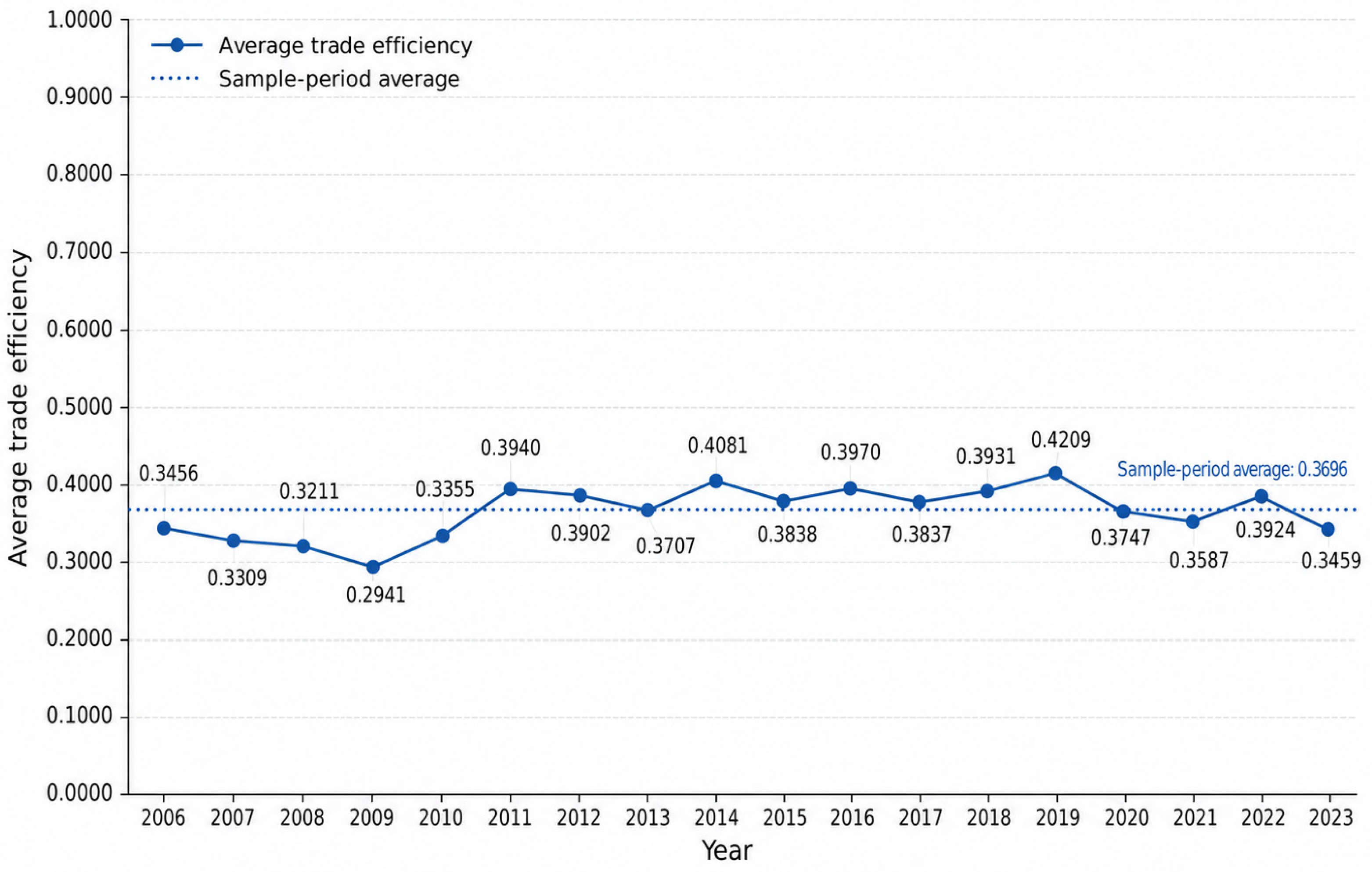
Figure 4 shows that during the sample period, the average trade efficiency of China’s aquatic product exports to 39 countries along the Belt and Road was 0.3696. This mean indicates a substantial average gap between observed exports and the estimated frontier export value, although it should not be interpreted as a directly realizable percentage increase in exports. Annual mean efficiency fluctuated over the sample period without a monotonic trend. Annual mean trade efficiency rebounded after 2010, remained comparatively high during 2011–2019, and declined after 2020 while continuing to fluctuate.

As shown in

Table 5. Average trade efficiency and ranking of China’s aquatic product exports to 39 countries along the Belt and Road, 2006–2023.

Rank	Country	Average Trade Efficiency	Observed Years	Rank	Country	Average Trade Efficiency	Observed Years
1	Israel	0.7981	18	21	Bulgaria	0.3685	18
2	Lithuania	0.7238	18	22	Slovenia	0.3138	18
3	Brunei †	0.7018	10	23	Egypt	0.2916	18
4	Ukraine †	0.6696	17	24	Vietnam	0.2730	18
5	Thailand	0.6432	18	25	Indonesia	0.1945	18
6	Latvia	0.6389	18	26	Oman	0.1764	18
7	Singapore	0.6325	18	27	Kuwait	0.1644	18
8	Poland	0.6236	18	28	Cambodia †	0.1523	17
9	Maldives †	0.5982	15	29	Qatar †	0.1113	17
10	Malaysia	0.5942	18	30	Bahrain	0.1035	18
11	Albania †	0.5592	15	31	Iran	0.0974	18
12	Estonia	0.5540	18	32	Saudi Arabia †	0.0858	17
13	United Arab Emirates	0.5480	18	33	Türkiye	0.0621	18
14	Croatia	0.5143	18	34	Syria †	0.0606	8
15	Philippines	0.5127	18	35	Bangladesh †	0.0112	16
16	Russia	0.5083	18	36	Yemen †	0.0091	5
17	Georgia †	0.4914	17	37	Myanmar †	0.0079	16
18	Jordan	0.4795	18	38	Pakistan	0.0004	18
19	Moldova †	0.4658	10	39	India	0.0004	18
20	Lebanon	0.4034	18
—	Overall Average	0.3696

Note: Country-level average trade efficiency is calculated over the available observations for each country during 2006–2023. Because the main sample is an unbalanced panel, the number of annual observations differs across countries. † indicates countries with fewer than 18 annual observations. Rankings are based on the unrounded trade-efficiency estimates. Source: Authors’ estimations based on the study dataset. Software: The models and statistical tests were estimated by the authors using Stata/MP 18.0.

, among destinations with complete 2006–2023 coverage, Israel, Lithuania, Thailand, Latvia, Singapore, Poland, Malaysia, Estonia, the United Arab Emirates, Croatia, the Philippines, Russia, Jordan, and Lebanon record comparatively high mean efficiency, placing their observed exports relatively close to the estimated frontier. Brunei, Ukraine, the Maldives, and Albania also rank relatively high, although their average efficiency values are based on fewer than 18 annual observations. By contrast, Indonesia, Oman, Kuwait, Bahrain, Iran, Türkiye, Pakistan, and India have comparatively low mean efficiency within the sample. Cambodia, Qatar, Saudi Arabia, Syria, Bangladesh, Yemen, and Myanmar also record relatively low average efficiency, but their rankings should be interpreted with consideration of their shorter temporal coverage.

5.2. Analysis of Export Trade Potential

Using the trade-efficiency estimates, this study further calculates the potential export values and expansion space of China’s aquatic product exports to 33 countries along the Belt and Road. Although the baseline model is estimated using 39 countries, only 33 countries have complete observations for all three years from 2021 to 2023 and are therefore included in the potential analysis. To reduce the impact of abnormal fluctuations in a single year on the results, this paper uses the average value of 2021–2023 for the calculation. The frontier export value is the observation-specific value implied by the stochastic frontier, while the frontier gap measures the difference between the estimated frontier export value and observed export value; neither measure is a demand forecast.

Table 6. Mean trade efficiency, observed export values, potential exports, and potential expansion ratios for 33 BRI destinations, 2021–2023.

Country	Trade Efficiency	Observed Exports (USD Million)	Potential Exports (USD Million)	Potential Expansion Ratio (Times)
Thailand	0.7847	1493.9327	1901.381	0.2727
Israel	0.7671	105.8978	137.8485	0.3017
Brunei	0.7482	4.6199	6.1596	0.3333
Estonia	0.7049	5.2076	7.3446	0.4104
Malaysia	0.6997	1493.6227	2131.9909	0.4274
Philippines	0.6358	914.5443	1431.036	0.5648
Maldives	0.6204	0.8602	1.3761	0.5998
Singapore	0.6141	254.0272	413.4816	0.6277
Albania	0.6058	2.4391	4.0077	0.6431
Jordan	0.6033	12.832	21.11	0.6451
Lebanon	0.5422	4.2127	7.573	0.7976
Latvia	0.5022	2.9916	5.6848	0.9002
United Arab Emirates	0.4892	39.6319	81.0129	1.0441
Lithuania	0.4785	4.4138	9.1882	1.0817
Poland	0.4158	63.9718	153.796	1.4041
Croatia	0.4125	3.4736	8.4174	1.4233
Vietnam	0.4045	462.8844	1144.3873	1.4723
Cambodia	0.3996	23.3762	58.1342	1.4869
Russia	0.3197	311.0797	977.5954	2.1426
Oman	0.2717	5.6706	20.8206	2.6717
Slovenia	0.214	0.9023	4.2168	3.6732
Bulgaria	0.2003	2.6004	12.7876	3.9175
Qatar	0.1983	3.337	16.7151	4.009
Indonesia	0.1636	214.8533	1304.8559	5.0732
Egypt	0.1218	26.7257	221.457	7.2863
Kuwait	0.053	1.0728	20.4461	18.0583
Türkiye	0.0506	15.9154	316.3359	18.8761
Bahrain †	0.0411	0.202	5.006	23.7835
Bangladesh †	0.0389	48.7431	1240.1855	24.4433
Iran †	0.0098	2.9456	299.4184	100.6504
Myanmar †	0.0073	1.2133	166.9463	136.5965
India †	0.0006	4.7997	7983.0419	1662.2409
Pakistan †	0.00004	0.03	746.8688	24,934.2444

Note: The values are averages for 2021–2023. All 33 countries have valid observations for each of the three years. The potential expansion ratio is calculated as (potential exports − observed exports)/observed exports. † indicates countries with trade efficiency below 0.05. Because potential exports are calculated using the inverse of estimated trade efficiency, potential export values and expansion ratios for countries with extremely low efficiency should be interpreted with caution. Source: Authors’ estimations based on the study dataset. Software: The models and statistical tests were estimated by the authors using Stata/MP 18.0.

shows that Thailand, Malaysia, the Philippines, Vietnam, Singapore, Russia, and Indonesia have relatively high observed export values, indicating that these countries are already important markets for China’s aquatic product exports. However, their trade efficiency differs considerably. Thailand, Malaysia, the Philippines, and Singapore have relatively high trade efficiency, with efficiency values ranging from 0.6141 to 0.7847, indicating that their observed exports are relatively close to the model-estimated frontier. By contrast, the trade efficiency of Vietnam, Russia, and Indonesia is 0.4045, 0.3197, and 0.1636, respectively. Despite their substantial export bases, these three markets remain relatively far from the estimated export frontier.

Table 6 shows that Bahrain, Bangladesh, Iran, Myanmar, India, and Pakistan have trade efficiencies below 0.05. Among these countries, the trade efficiency of India and Pakistan is close to zero, and their potential export estimates should therefore be interpreted with particular caution. The low trade efficiency of these two countries may reflect omitted or imperfectly measured constraints, including local supply capacity, bilateral relations, consumer demand, and market access conditions. India has a strong domestic supply and export capacity for aquatic products, which may reduce its import demand for similar products [33]. Fluctuations in China–India political relations may also increase uncertainty in bilateral trade [34]. Pakistan has relatively low per capita fish consumption, which may limit domestic import demand. Pakistan’s aquatic product trade with China has long been dominated by exports to China [12]. Processed aquatic products entering markets such as Pakistan may need to satisfy halal certification, processing procedures, and supply chain integrity requirements [35,36]. These conditions may be associated with lower observed exports from China and larger estimated frontier gaps. Because the frontier value is calculated as observed exports divided by estimated efficiency, efficiency values near zero mechanically produce very large frontier estimates. These estimates should therefore not be interpreted as export increments achievable in the short term.

5.3. Export Market Classification Matrix

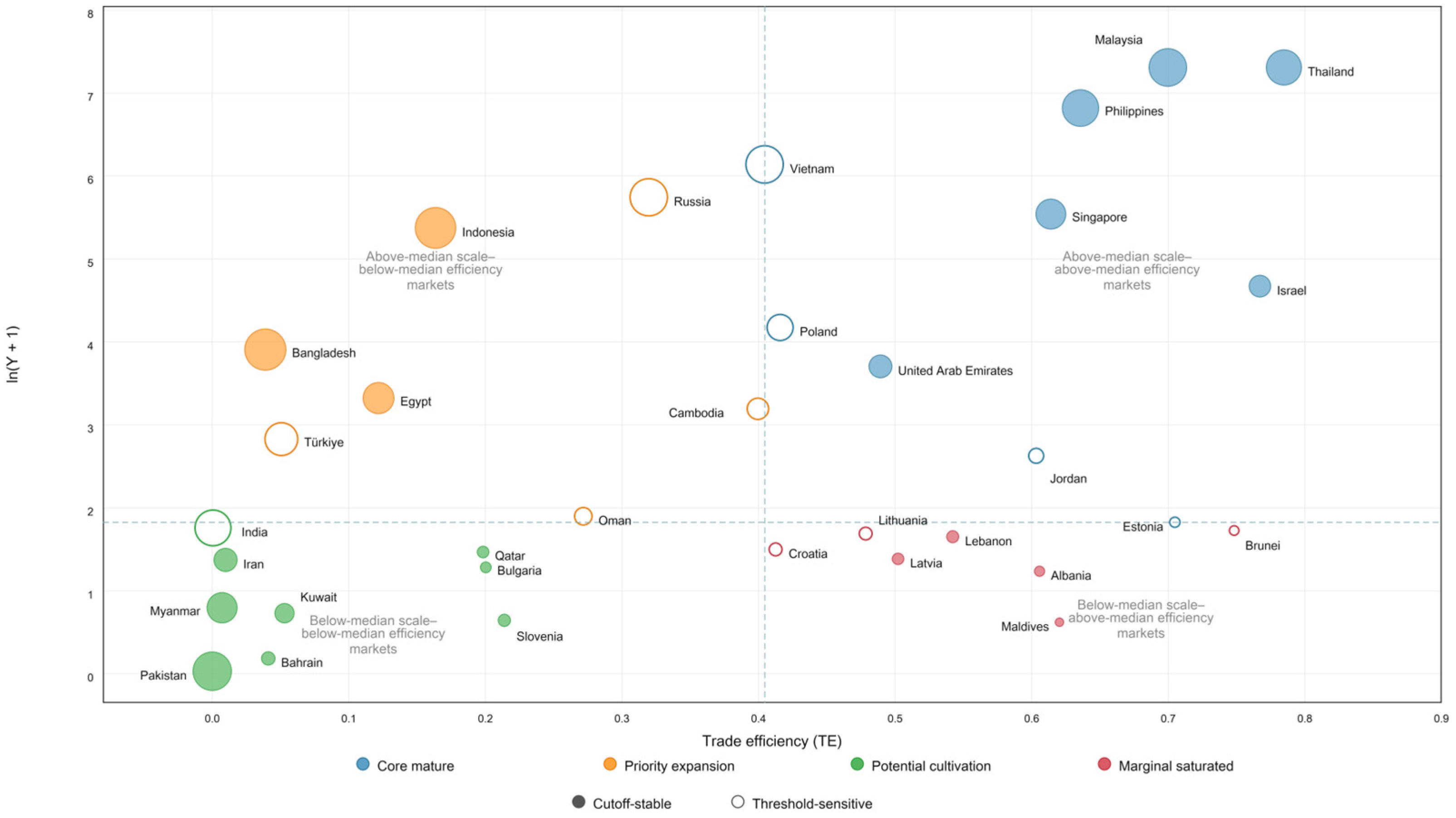
Based on the results reported in Table 6, this study constructs an export market classification matrix using data for the 33 countries with valid observations in each year from 2021 to 2023. Following the country-market portfolio logic commonly used in international market analysis, this study combines observed export scale and trade efficiency to construct a two-dimensional descriptive matrix [37,38]. Trade efficiency ($TE$) is plotted on the horizontal axis, while the natural logarithm of observed exports plus one, ln(Y + 1), is placed on the vertical axis, where Y denotes the mean observed export value (USD million) for 2021–2023. Observed exports capture the realized commercial scale of each market, whereas trade efficiency measures the extent to which observed exports approach the model-estimated frontier. Considering these two dimensions jointly helps distinguish small markets with large relative frontier gaps from larger markets in which improvements in trade efficiency may generate more substantial absolute export gains. Bubble size represents the export-potential gap, which is used as supplementary information rather than as a criterion for quadrant assignment.

In Figure 5, the sample medians of trade efficiency and observed exports, 0.4045 and USD 5.208 million, respectively, are used to divide the 33 markets into four relative groups. The export-value median corresponds to ln(Y + 1) = 1.8258, with the logarithmic scale used only to improve graphical readability. The sample medians are used as robust, data-centered reference points rather than as economically optimal thresholds. This choice reflects the highly right-skewed distribution of observed exports across the 33 markets: the mean export value is USD 167.668 million, compared with a median of USD 5.208 million, while the five largest markets account for 84.51% of total exports within the classification sample. Because the median is less sensitive to extreme values than the mean, it provides a more representative benchmark for relative comparisons within this sample [39]. To assess the sensitivity of the classification to the cutoff rule, the market groups are recalculated using the 40th and 60th percentiles as alternatives to the sample medians [40]. Across the three cutoff rules, 21 of the 33 markets remain in the same category, whereas 12 change category under at least one alternative rule. The detailed results are reported in Table S4 of the Supplementary Materials.

Under the median-based descriptive classification shown in Figure 5, the 33 destinations form four groups of export markets. (1) Above-median scale–above-median efficiency markets include countries such as Thailand, Malaysia, and the Philippines. China’s aquatic products export values to these markets is large and trade efficiency is high, with a relatively stable market foundation. (2) Above-median scale–below-median efficiency markets include countries such as Indonesia, Egypt, and Bangladesh. China’s aquatic product exports to these countries have reached a certain scale, but trade efficiency remains relatively low, indicating a gap between observed exports and the estimated frontier. (3) Below-median scale–below-median efficiency markets include countries such as Slovenia, Bulgaria, and Qatar. These markets have both below-median observed exports and below-median efficiency. (4) Below-median scale–above-median efficiency markets include countries such as the Maldives, Albania, and Latvia. These markets have above-median efficiency but below-median export scale. The classifications of the 12 markets represented by hollow bubbles in Figure 5 are sensitive to the choice of percentile cutoff and should therefore be interpreted as relative positions under the median-based classification rather than as fixed market categories.

6. Robustness Test

6.1. Robustness Tests of the Baseline BC95 Model

To verify the reliability of the results of preferred BC95 model, this paper conducts robustness tests in three ways: excluding the observations from 2020 to 2022, when international trade was more directly affected by pandemic-related disruptions; winsorizing the dependent variable and the continuous time-varying covariates at the 1st and 99th percentiles; and lagging the time-varying inefficiency covariates by one year. The test results are shown in

Table 7. Robustness checks for the preferred BC95 specification.

Variable	Baseline Model	Excluding 2020–2022	Winsorization	One-Period-Lagged Inefficiency Variables
Stochastic Frontier Equation
$\ln {\mathrm{G}\mathrm{D}\mathrm{P}}_{\mathrm{i}\mathrm{t}}$	0.4598 ***	0.5108 ***	0.4504 ***	0.4428 ***
	(5.2416)	(5.0727)	(5.1428)	(4.2327)
$\ln {\mathrm{G}\mathrm{D}\mathrm{P}}_{j\mathrm{t}}$	0.6345 ***	0.6450 ***	0.6547 ***	0.6175 ***
	(9.5580)	(8.6636)	(9.8073)	(8.8792)
$\ln {\mathrm{P}\mathrm{O}\mathrm{P}}_{\mathrm{j}\mathrm{t}}$	0.5666 ***	0.5622 ***	0.5528 ***	0.5696 ***
	(8.7776)	(7.6361)	(8.5630)	(8.4069)
$\ln {Dist}_{ij}$	−1.5842 ***	−1.3220 ***	−1.5666 ***	−1.6723 ***
	(−8.5612)	(−6.4009)	(−8.5863)	(−8.7443)
${Comlang}_{ij}$	1.5922 ***	1.6119 ***	1.5571 ***	1.5992 ***
	(8.9854)	(8.2781)	(8.8133)	(8.6839)
$\mathrm{c}\mathrm{o}\mathrm{n}\mathrm{s}.$	−8.0167 **	−11.9810 ***	−8.1658 **	−6.3663
	(−2.2992)	(−3.0475)	(−2.3456)	(−1.6046)
Trade Inefficiency Equation
${FTA}_{ijt}$	−0.8086	−0.8336	−0.7232	−0.7289
	(−0.8536)	(−0.8276)	(−0.8137)	(−0.7424)
${PS}_{jt}$	−2.8983 ***	−2.5563 ***	−2.7257 ***	−2.8348 ***
	(−3.7406)	(−3.3319)	(−3.7402)	(−3.5975)
${GE}_{jt}$	−2.5978 **	−2.5433 **	−2.2803 **	−3.0389 **
	(−2.2214)	(−2.0948)	(−2.1291)	(−2.4416)
$\ln {MF}_{jt}$	5.4639	4.0067	5.1658	7.8545 *
	(1.3876)	(0.9198)	(1.2808)	(1.6976)
$\ln {TF}_{jt}$	−7.7996 ***	−6.9291 ***	−7.4019 ***	−7.1242 ***
	(−2.9853)	(−2.6225)	(−2.6238)	(−2.6878)
$\ln {FF}_{jt}$	−0.2961	−0.0286	−0.3635	−0.5028
	(−0.2767)	(−0.0259)	(−0.3568)	(−0.4560)
$\ln {LSCI}_{jt}$	−0.6489	−0.9923	−0.4865	−0.8906
	(−1.0556)	(−1.5388)	(−0.8425)	(−1.4037)
$\ln {PROD}_{jt}$	1.0134 ***	0.9743 ***	0.8916 ***	1.0594 ***
	(3.4832)	(3.1976)	(3.3738)	(3.4644)
${HALAL}_j$	5.1442 ***	5.2510 ***	4.7291 ***	5.2504***
	(4.4470)	(4.2066)	(4.4842)	(4.3327)
$\mathrm{c}\mathrm{o}\mathrm{n}\mathrm{s}.$	−7.2660	−3.1521	−5.6062	−19.2212
	(−0.3766)	(−0.1486)	(−0.2822)	(−0.8774)
${\sigma }^2$	14.8011 ***	14.2146 ***	13.6336 ***	14.7511 ***
	(4.8348)	(4.4827)	(4.9403)	(4.6695)
$\gamma$	0.9781 ***	0.9771 ***	0.9777 ***	0.9778 ***
	(161.8255)	(143.8400)	(157.8282)	(153.9406)
Log likelihood	−1138.6230	−953.4628	−1133.8746	−1071.8170
$LR$ statistic	461.3852	831.7064	470.8820	594.9972
Mean trade efficiency	0.3696	0.3633	0.3656	0.3713
Observations	648	539	648	611

Note: The values in parentheses are z-statistics. *, **, *** indicate statistical significance at the 10%, 5%, and 1% levels, respectively. Source: Authors’ estimations based on the study dataset. Software: The models and statistical tests were estimated by the authors using Stata/MP 18.0.

. As a stricter temporal sensitivity test, the model is also re-estimated after excluding all observations from 2020 to 2023, with the results reported in Table S5 of the Supplementary Materials.

Across these tests, the signs and significance of the frontier variables remain stable. Political stability, government effectiveness, and trade freedom remain significantly associated with lower trade inefficiency, while destination-country aquatic product production and halal certification requirements remain significantly associated with higher trade inefficiency. The estimated mean trade efficiency and γ also remain close to the baseline estimates. In the stricter exclusion test, liner shipping connectivity becomes significant only at the 10% level, indicating some sensitivity, while the other principal results remain unchanged. Overall, the main findings are not materially altered by excluding the pandemic-period observations, winsorizing extreme values, or lagging the time-varying inefficiency covariates.

6.2. Alternative Sample and Model Specifications

To assess whether the results depend on sample composition, the assumed inefficiency distribution, or the estimation method, two additional sets of robustness checks are conducted. First, the BC95 model is re-estimated using the 26-country balanced panel and an alternative exponential inefficiency distribution. Second, the gravity equation is re-estimated using positive-flow PPML and a Log-OLS specification with importer and year fixed effects. The results are reported in

Table 8. Results of alternative sample and model specifications.

Variable	Baseline Model	26-Country Balanced Panel	Exponential Distribution	Positive-Flow PPML	Log-OLS with Importer and Year Fixed Effects
Stochastic Frontier Equation
$\ln {GDP}_{it}$	0.4598 ***	0.4256 ***	0.4947 ***	0.4924 *	Absorbed
	(5.2416)	(4.7257)	(5.7341)	(1.77)
$\ln {GDP}_{jt}$	0.6345 ***	0.8021 ***	0.6073 ***	0.9705 **	1.5549 ***
	(9.5580)	(11.1315)	(6.7469)	(2.40)	(2.93)
$\ln {POP}_{jt}$	0.5666 ***	0.5371 ***	0.6038 ***	−0.2508	0.9655
	(8.7776)	(6.6823)	(6.5249)	(−0.81)	(1.10)
$\ln {Dist}_{ij}$	−1.5842 ***	−1.4707 ***	−1.5654 ***	−2.6734 ***	Absorbed
	(−8.5612)	(−6.3965)	(−8.1418)	(−3.00)
${Comlang}_{ij}$	1.5922 ***	1.5466 ***	1.6864 ***	1.1841	Absorbed
	(8.9854)	(8.5114)	(7.8969)	(1.38)
$\mathrm{c}\mathrm{o}\mathrm{n}\mathrm{s}.$	−8.0167 **	−11.9976 ***	−9.4483 ***	4.7333	−40.0047 **
	(−2.2992)	(−3.0799)	(−2.8119)	(0.63)	(−2.52)
Trade Inefficiency Equation
${FTA}_{ijt}$	−0.8086	−7.7877 ***	−0.3284 *	—	—
	(−0.8536)	(−2.8110)	(−1.9223)
${PS}_{jt}$	−2.8983 ***	−8.8350 ***	−0.2246 **	—	—
	(−3.7406)	(−3.3126)	(−2.5316)
${GE}_{jt}$	−2.5978 **	−0.1443	−0.3153 *	—	—
	(−2.2214)	(−0.0654)	(−1.6807)
$\ln {MF}_{jt}$	5.4639	10.5123	0.4126	—	—
	(1.3876)	(1.2966)	(0.7418)
$\ln {TF}_{jt}$	−7.7996 ***	−15.6894 ***	−1.1463 ***	—	—
	(−2.9853)	(−3.0631)	(−2.7795)
$\ln {FF}_{jt}$	−0.2961	3.1257	−0.1836	—	—
	(−0.2767)	(1.3865)	(−0.7419)
$\ln {LSCI}_{jt}$	−0.6489	−3.7905 *	−0.1140	—	—
	(−1.0556)	(−1.8407)	(−1.0018)
$\ln {PROD}_{jt}$	1.0134 ***	2.9858 ***	0.1484 *	—	—
	(3.4832)	(2.8566)	(1.9576)
${HALAL}_j$	5.1442 ***	6.7620 ***	0.8862 ***	—	—
	(4.4470)	(2.8636)	(4.7576)
$\mathrm{c}\mathrm{o}\mathrm{n}\mathrm{s}.$	−7.2660	−27.2755	2.4945	—	—
	(−0.3766)	(−0.6549)	(0.7881)
${\sigma }^2$	14.8011 ***	20.2324 ***	—	—	—
	(4.8348)	(3.1547)
$\gamma$	0.9781 ***	0.9795 ***	—	—	—
	(161.8255)	(124.9115)
Log likelihood	−1138.6230	−776.4076	—	—	—
Observations	648	468	648	648	648
Countries	39	26	39	39	39
Mean trade efficiency	0.3696	0.4510	0.4595	—	—
Year fixed effects	No	No	No	No	Yes
Importer fixed effects	No	No	No	No	Yes
Spearman rank correlation	—	0.9809	0.9605	—	—
Kendall rank correlation	—	0.9077	0.8839	—	—

Note: The 26-country balanced-panel specification retains the full set of variables used in the baseline BC95 model but restricts the sample to countries with complete observations for all 18 years. The exponential specification uses the 39-country unbalanced sample and replaces the truncated-normal inefficiency distribution with an exponential distribution. The positive-flow PPML specification is estimated using the 39-country unbalanced sample with recorded positive export observations, whereas the Log-OLS specification includes importer and year fixed effects. PPML and Log-OLS are alternative gravity-model comparisons and do not estimate a separate trade inefficiency equation. Dashes indicate results that are not reported or not applicable; ‘Absorbed’ indicates regressors that are collinear with the included fixed effects. The Spearman and Kendall coefficients report the correlations between country-level trade-efficiency rankings obtained from each alternative specification and those from the baseline model. Values in parentheses are z statistics. ***, **, and * indicate significance at the 1%, 5%, and 10% levels, respectively. Source: Authors’ estimations based on the study dataset. Software: The models and statistical tests were estimated by the authors using Stata/MP 18.0.

.

The stochastic-frontier estimates in Table 8 shows that the principal results are robust to changes in sample composition and the assumed inefficiency distribution. Exporter GDP, destination-country GDP, destination-country population, and common language remain positively and significantly associated with the trade frontier, while geographical distance remains negatively and significantly associated with it. In the inefficiency equation, political stability and trade freedom remain negatively and significantly associated with trade inefficiency, whereas destination-country aquatic product production and halal certification requirements remain positively and significantly associated with it. These associations are the most stable across the alternative stochastic-frontier specifications. By contrast, free trade agreements, government effectiveness, and liner shipping connectivity are more sensitive to model specification because their statistical significance varies across the alternative specifications, while monetary freedom and financial freedom show no consistent statistically significant associations. The country-level efficiency rankings also remain highly stable, with Spearman correlations of 0.9809 and 0.9605 and Kendall correlations of 0.9077 and 0.8839. In addition, 23 of the 26 common countries retain the same market classification. However, differences in mean trade efficiency indicate that relative country rankings are more robust than absolute efficiency levels.

Table 8 also reports the results from two alternative gravity specifications. The coefficient of destination-GDP remains positive and statistically significant in both alternative gravity specifications, supporting a robust association with destination market size. The PPML estimates also retain a positive coefficient on exporter GDP and a negative coefficient on distance. In the Log-OLS model, exporter GDP is absorbed by year fixed effects, whereas geographical distance and common language are absorbed by importer fixed effects. By contrast, the coefficients on destination-country population and shared official language are more sensitive to model specification.

7. Conclusions and Policy Implications

7.1. Conclusions

Using an unbalanced panel of China’s aquatic product exports to 39 countries along the Belt and Road from 2006 to 2023, this study applies the BC95 one-step stochastic frontier gravity model to estimate trade efficiency, identify the factors associated with the trade frontier and trade inefficiency, assess country-level export potential, and classify destination markets according to export scale and trade efficiency. The main conclusions corresponding to these four research objectives are as follows.

First, significant inefficiency exists in China’s aquatic product exports to the sample countries. The mean trade efficiency over the sample period is 0.3696, indicating a substantial average gap between observed exports and the model-estimated trade frontier. Annual trade efficiency does not follow a monotonic upward or downward trend. It recovered after 2010, remained relatively high from 2011 to 2019, and declined and fluctuated after 2020. Country-level estimates also vary considerably. China’s exports to Israel, Lithuania, Thailand, Latvia, Singapore, Poland, and Malaysia are relatively close to the estimated frontier, whereas exports to Indonesia, Oman, Kuwait, Türkiye, Iran, Pakistan, and India exhibit relatively low efficiency. These results show that the overall expansion of China’s aquatic product exports has not been accompanied by a uniform improvement in trade efficiency across destination markets.

Second, the factors associated with the trade frontier differ from those associated with trade inefficiency. In the baseline frontier equation, China’s GDP, importing-country GDP and population, and common language are positively associated with exports, whereas geographical distance is negatively associated with exports. Importing-country GDP remains positive and statistically significant in both alternative gravity specifications, confirming the importance of destination-market size. The PPML results also support the positive association of China’s GDP and the negative association of geographical distance with exports. By contrast, the estimates for importing-country population and common language are more sensitive to model specification. In the inefficiency equation, political stability and trade freedom are consistently associated with lower trade inefficiency, whereas importing-country aquatic product production and halal certification requirements are consistently associated with higher trade inefficiency across the principal robustness tests. Government effectiveness, free trade agreements, and liner shipping connectivity are more sensitive to changes in the sample or model specification, while monetary freedom and financial freedom are statistically insignificant in most specifications. The findings indicate that economic scale helps determine the attainable trade frontier, while institutional conditions, local supply capacity, and market-access requirements affect the extent to which that frontier is realized.

Third, substantial cross-country differences are found in model-estimated export potential. Among the 33 countries with complete observations for 2021–2023, markets with similar export scales can occupy markedly different efficiency positions. Thailand, Malaysia, the Philippines, and Singapore combine relatively large export values with comparatively high trade efficiency, whereas Vietnam, Russia, and Indonesia have substantial export bases but remain farther from the estimated frontier. The potential estimates for countries with extremely low efficiency, particularly India and Pakistan, require greater caution. Because potential exports are calculated by dividing observed exports by estimated trade efficiency, efficiency values close to zero mechanically produce exceptionally large potential estimates. These estimates represent statistical gaps from the model-estimated frontier rather than export increases that can be achieved in the short term. Their practical interpretation must therefore take into account actual import demand, domestic aquatic product supply, bilateral relations, consumer preferences, certification requirements, and other market-access conditions.

Fourth, the scale–efficiency matrix classifies the 33 destination markets into four sample-relative groups: above-median scale–above-median efficiency, above-median scale–below-median efficiency, below-median scale–below-median efficiency, and below-median scale–above-median efficiency. The model-estimated export-potential gap provides supplementary information on each market’s distance from the estimated frontier but does not determine group membership. The sensitivity analysis shows that 21 markets retain the same classification under the 40th-percentile, median, and 60th-percentile cutoff rules, whereas 12 markets change group under at least one alternative threshold. The classification therefore provides a differentiated description of the relative positions of destination markets, but the results for markets located near the thresholds should not be treated as fixed judgments of market maturity, saturation, or expansion priority.

Taken together, the main findings show that the growth of China’s aquatic product exports to countries along the Belt and Road cannot be evaluated solely by export value or estimated potential. A large destination market may raise the attainable export frontier, but the realization of that frontier also depends on political stability, trade openness, local aquatic product supply, certification requirements, and other market-specific conditions. Moreover, a large model-estimated potential does not necessarily indicate a readily accessible market, particularly when the estimate is driven by extremely low trade efficiency. The central finding is therefore that the sustainable development of China’s aquatic product exports requires a shift from uniform scale expansion toward differentiated market strategies that place greater emphasis on trade efficiency, institutional conditions, compliance capacity, and the practical feasibility of converting estimated potential into realized trade.

7.2. Policy Implications

Based on the findings of this study, China’s aquatic product exports should shift from a scale-expansion-oriented model to a sustainable trade development model that places greater emphasis on efficiency, product quality, regulatory compliance and trade stability. Such a shift requires coordinated action at the national, industry, and firm levels.

At the national level, institutional support and public services for sustainable aquatic products trade should be strengthened. Greater attention should be paid to differences in political stability, trade freedom, local aquatic product supply, and certification requirements across destination countries. Country-specific risk monitoring and early-warning mechanisms, market information services, and trade risk-mitigation instruments should be strengthened, alongside certification support for markets where halal or other product-specific requirements apply. Port cold-chain infrastructure, customs clearance, and related logistics services should also be improved to mitigate trade frictions related to geographical distance. Based on the scale–efficiency classification and the model-estimated export potential, market support policies should be differentiated across countries, rather than using the calculated potential directly as a basis for expanding exports.

At the industry level, logistics organization, certification services, and market service capabilities should be strengthened. Aquatic product industry associations and relevant service institutions should provide firms with information and support on cold-chain transportation, certification requirements, and market access conditions, with particular attention paid to markets subject to halal certification requirements. An industry database covering destination market demand, local aquatic product supply, certification requirements, and market access conditions could support decisions across market types and improve resource allocation.

At the firm level, decision making should shift from export value alone toward trade efficiency and responsiveness to destination-market requirements. Enterprises should select export markets by considering observed market demand, local aquatic product supply, certification requirements, and the estimated trade efficiency, rather than relying solely on model-estimated export potential. For above-median scale–above-median efficiency markets, the priority should be to maintain existing trade relationships and market positions. For above-median scale–below-median efficiency markets, enterprises should identify the constraints associated with relatively low trade efficiency before further expanding exports. For below-median scale–below-median efficiency markets, firms should assess demand and access conditions before undertaking gradual, small-scale market development. For below-median scale–above-median efficiency markets, enterprises should maintain existing trade relationships while taking into account the relatively limited export scale. For markets whose classifications change under alternative cutoff rules, market strategies should not rely on a single classification result.

7.3. Limitations

This study is subject to limitations arising from data coverage. Although the initial candidate frame contains 64 Belt and Road countries, unavailable export records and covariate data reduce the preferred estimation sample to an unbalanced panel of 39 countries. Complete-case selection may be non-random if the availability of recorded exports or covariates is associated with trade frictions, maritime connectivity, or national reporting capacity. Potential sample-selection bias therefore cannot be ruled out. The estimates should be interpreted as applying to recorded positive-flow country-year observations with complete covariate data in the 39 included markets, rather than as fully representative of all 64 candidate countries or of unreported trade relationships. The balanced-panel sensitivity analysis provides evidence on the stability of the efficiency rankings across alternative sample structures, but it cannot determine the values or characteristics of the unavailable observations.

References

1. Crona, B.I.; Wassénius, E.; Jonell, M.; Koehn, J.Z.; Short, R.; Tigchelaar, M.; Daw, T.M.; Golden, C.D.; Gephart, J.A.; Allison, E.H.; et al. Four ways blue foods can help achieve food system ambitions across nations. Nature 2023, 616, 104–112. [Google Scholar] [CrossRef] [Scilit] [PubMed]
2. Yang, B.; Anderson, J.L.; Asche, F. Determinants of China’s seafood trade patterns. Mar. Resour. Econ. 2020, 35, 97–112. [Google Scholar] [CrossRef] [Scilit]
3. Xi, J. Hold High the Great Banner of Socialism with Chinese Characteristics and Strive in Unity to Build a Modern Socialist Country in All Respects: Report to the 20th National Congress of the Communist Party of China. Available online: https://english.www.gov.cn/news/topnews/202210/25/content_WS6357df20c6d0a757729e1bfc.html (accessed on 23 July 2026).
4. Ministry of Agriculture and Rural Affairs of the People’s Republic of China. The 14th Five-Year Plan for National Fisheries Development. Available online: https://yyj.moa.gov.cn/gzdt/202201/t20220107_6386443.htm (accessed on 23 July 2026). (In Chinese)
5. Djankov, S.; Freund, C.; Pham, C.S. Trading on time. Rev. Econ. Stat. 2010, 92, 166–173. [Google Scholar] [CrossRef] [Scilit]
6. Liu, L.; Yue, C. Investigating the impacts of time delays on trade. Food Policy 2013, 39, 108–114. [Google Scholar] [CrossRef] [Scilit]
7. Dey, M.M.; Rab, M.A.; Jahan, K.M.; Nisapa, A.; Kumar, A.; Ahmed, M. Food safety standards and regulatory measures: Implications for selected fish exporting Asian countries. Aquac. Econ. Manag. 2005, 9, 217–236. [Google Scholar] [CrossRef] [Scilit]
8. Malcorps, W.; Newton, R.W.; Maiolo, S.; Eltholth, M.; Zhu, C.; Zhang, W.; Li, S.; Tlusty, M.; Little, D.C. Global seafood trade: Insights in sustainability messaging and claims of the major producing and consuming regions. Sustainability 2021, 13, 11720. [Google Scholar] [CrossRef] [Scilit]
9. Nisar, U.; Zhang, Z.; Cui, Z.; Mu, Y.; Zhang, H. Impact of COVID-19 on fish and crustacean export from China with building resilient food system through China’s lens. Front. Sustain. Food Syst. 2023, 7, 1189526. [Google Scholar] [CrossRef] [Scilit]
10. Natale, F.; Borrello, A.; Motova, A. Analysis of the determinants of international seafood trade using a gravity model. Mar. Policy 2015, 60, 98–106. [Google Scholar] [CrossRef] [Scilit]
11. Miao, M.; Liu, H.; Chen, J. Factors affecting fluctuations in China’s aquatic product exports to Japan, the USA, South Korea, Southeast Asia, and the EU. Aquac. Int. 2021, 29, 2507–2533. [Google Scholar] [CrossRef] [Scilit] [PubMed]
12. Xia, Y.; Yin, H.; Mohsin, M.; Mehak, A.; Yan, C. Exploring FTAs, seafood exports, and SDGs: A gravity model analysis of Pakistan’s seafood trade with China and regional partners. Front. Mar. Sci. 2025, 12, 1553780. [Google Scholar] [CrossRef] [Scilit]
13. Shan, S.; Yan, Y. Trade facilitation and sustainable agricultural trade in the RCEP: Empirical evidence from China’s heterogeneous impacts. Sustainability 2025, 17, 7640. [Google Scholar] [CrossRef] [Scilit]
14. Cai, Y.; Chen, W.; Zeng, X. The impact of the depth of environmental provisions in regional trade agreements on China’s fisheries and aquaculture trade. Front. Sustain. Food Syst. 2026, 10, 1741505. [Google Scholar] [CrossRef] [Scilit]
15. Liu, H.; Zhang, S.; Mu, Y.; Zhu, Y. Topology and evolution of international trade network for fish and fish products. Front. Sustain. Food Syst. 2023, 7, 1134687. [Google Scholar] [CrossRef] [Scilit]
16. Liu, W.; Yang, Y. Development characteristics and pathways of aquatic product trade between China and RCEP member countries. Issues Agric. Econ. 2024, 11, 127–144. (In Chinese) [Google Scholar]
17. Anderson, J.E. A theoretical foundation for the gravity equation. Am. Econ. Rev. 1979, 69, 106–116. [Google Scholar]
18. Anderson, J.E.; van Wincoop, E. Gravity with gravitas: A solution to the border puzzle. Am. Econ. Rev. 2003, 93, 170–192. [Google Scholar] [CrossRef] [Scilit]
19. Aigner, D.; Lovell, C.A.K.; Schmidt, P. Formulation and estimation of stochastic frontier production function models. J. Econom. 1977, 6, 21–37. [Google Scholar] [CrossRef] [Scilit]
20. Battese, G.E.; Coelli, T.J. A model for technical inefficiency effects in a stochastic frontier production function for panel data. Empir. Econ. 1995, 20, 325–332. [Google Scholar] [CrossRef] [Scilit]
21. Abdullahi, N.M.; Zhang, Q.; Shahriar, S.; Irshad, M.S.; Ado, A.B.; Huo, X. Examining the determinants and efficiency of China’s agricultural exports using a stochastic frontier gravity model. PLoS ONE 2022, 17, e0274187. [Google Scholar] [CrossRef] [Scilit] [PubMed]
22. Shi, L.; Zhang, S.; Hashmi, S.M. Study on the export pattern and export potential of agricultural products from China to RCEP countries—An empirical study based on gravity model. Front. Sustain. Food Syst. 2025, 9, 1492812. [Google Scholar] [CrossRef] [Scilit]
23. Du, J.; Liu, Y.; Luo, S.; Luo, X. A study on the trade efficiency and potential of China’s agricultural products export to Association of South East Asian Nations countries: Empirical analysis based on segmented products. Agriculture 2024, 14, 1387. [Google Scholar] [CrossRef] [Scilit]
24. Romyen, A.; Nunti, C.; Neranon, P. Trade efficiency under FTA for Thailand’s agricultural exports: Copula-based gravity stochastic frontier model. J. Econ. Struct. 2023, 12, 9. [Google Scholar] [CrossRef] [Scilit]
25. Cao, F.; Li, X.; Zhang, Z. Does institutional openness improve the trade efficiency of China’s agricultural products imported from Central Asian countries? A time-varying stochastic frontier gravity model. Front. Sustain. Food Syst. 2025, 9, 1598004. [Google Scholar] [CrossRef] [Scilit]
26. Battese, G.E.; Coelli, T.J. Frontier production functions, technical efficiency and panel data: With application to paddy farmers in India. J. Prod. Anal. 1992, 3, 153–169. [Google Scholar] [CrossRef] [Scilit]
27. Xing, L.; Yin, X.; Cao, C.; Elahi, E.; Wei, T. The Impact of Multidimensional Distance on Agricultural Exports: Evidence from China Based on the Technological Added Value. Sustainability 2023, 15, 393. [Google Scholar] [CrossRef] [Scilit]
28. Miao, T.; Pastpipatkul, P.; Liu, X.; Liu, J. The trade potential of grain crops in the countries along the Belt and Road: Evidence from a stochastic frontier model. Front. Sustain. Food Syst. 2024, 8, 1404232. [Google Scholar] [CrossRef] [Scilit]
29. Francois, J.; Manchin, M. Institutions, infrastructure, and trade. World Dev. 2013, 46, 165–175. [Google Scholar] [CrossRef] [Scilit]
30. Chen, H.; Qi, C. The trade effect of trust: Evidence from agricultural trade between China and its partners. Sustainability 2022, 14, 729. [Google Scholar] [CrossRef] [Scilit]
31. Ferreira, J.-P.; Garlock, T.M.; Court, C.D.; Anderson, J.L.; Asche, F. The economic contribution of U.S. seafood imports throughout the value chain: A sectorial and species-specific analysis. Mar. Policy 2024, 169, 106375. [Google Scholar] [CrossRef] [Scilit]
32. Limenta, M.; Edis, B.M.; Fernando, O. Disabling labelling in Indonesia: Invoking WTO laws in the wake of halal policy objectives. World Trade Rev. 2018, 17, 451–476. [Google Scholar] [CrossRef] [Scilit]
33. Villanthenkodath, M.A.; Pal, S. Assessing the relative impact of inland and marine fish production on fishing load capacity factor: Insights for sustainable fisheries management. Mar. Pollut. Bull. 2025, 215, 117855. [Google Scholar] [CrossRef] [Scilit] [PubMed]
34. Agarwal, V.; Golley, J. Do political relations affect exports to China? Evidence from the ‘Quad’. World Econ. 2022, 45, 2882–2901. [Google Scholar] [CrossRef] [Scilit]
35. Demirci, M.N.; Soon, J.M.; Wallace, C.A. Positioning food safety in Halal assurance. Food Control 2016, 70, 257–270. [Google Scholar] [CrossRef] [Scilit]
36. van der Spiegel, M.; Van der Fels-Klerx, H.J.; Sterrenburg, P.; van Ruth, S.M.; Scholtens-Toma, I.M.J.; Kok, E.J. Halal assurance in food supply chains: Verification of halal certificates using audits and laboratory analysis. Trends Food Sci. Technol. 2012, 27, 109–119. [Google Scholar] [CrossRef] [Scilit]
37. Ayal, I.; Peer, A.; Zif, J. Selecting industries for export growth—A directional policy matrix approach. J. Macromark. 1987, 7, 22–33. [Google Scholar] [CrossRef] [Scilit]
38. Douglas, S.P.; Craig, C.S. Executive Insights: Global Portfolio Planning and Market Interconnectedness. J. Int. Mark. 1996, 4, 93–110. [Google Scholar] [CrossRef] [Scilit]
39. Rousseeuw, P.J. Tutorial to robust statistics. J. Chemom. 1991, 5, 1–20. [Google Scholar] [CrossRef] [Scilit]
40. Azzopardi, E.; Nash, R. A critical evaluation of importance–performance analysis. Tour. Manag. 2013, 35, 222–233. [Google Scholar] [CrossRef] [Scilit]
Figure 1. Value of China’s aquatic product exports to the 39 sample countries and their share of China’s total aquatic product exports from 2006 to 2023. Note: Source: Authors’ calculations based on UN Comtrade data. Software: The figure was prepared by the authors using Microsoft Excel.
Sustainability 18 09404 g001
Figure 2. Value and share of China’s aquatic product exports to the 39 sample countries along the Belt and Road by product category from 2006 to 2023. Note: Source: Authors’ calculations based on UN Comtrade data. Software: The figure was prepared by the authors using Microsoft Excel.
Sustainability 18 09404 g002
Figure 3. Average value of China’s aquatic product exports to the 39 sample countries along the Belt and Road by product category from 2021 to 2023. Note: Source: Authors’ calculations based on UN Comtrade data. Software: The figure was prepared by the authors using Microsoft Excel.
Sustainability 18 09404 g003
Figure 4. Annual average trade efficiency of China’s aquatic product exports to the 39 sample countries along the Belt and Road from 2006 to 2023. Note: Source: Authors’ calculations based on trade-efficiency estimates from the preferred BC95 model. Software: Trade efficiency was estimated using Stata/MP 18.0, and the figure was prepared by the authors using Microsoft Excel.
Sustainability 18 09404 g004
Figure 5. Scale-efficiency matrix for 33 BRI destination markets. Note: The horizontal axis represents trade efficiency ( T E ), and the vertical axis represents ln(Y + 1), where Y denotes the average observed export value in USD million during 2021–2023. Bubble size represents the model-estimated export potential gap, calculated as the difference between potential exports and observed exports. The dashed lines mark the sample medians of T E (0.4045) and ln(Y + 1) (1.8258), which are used as descriptive rather than economically determined cutoffs. Filled bubbles indicate markets whose classifications remain unchanged under the 40th-percentile, median, and 60th-percentile cutoff rules, whereas hollow bubbles indicate threshold-sensitive markets. Source: Authors’ calculations based on UN Comtrade data and trade-efficiency estimates from the preferred BC95 model. Software: Trade efficiency and export potential were estimated using Stata/MP 18.0, and the figure was prepared by the authors using Python 3.13.5.
Sustainability 18 09404 g005