Spatiotemporal Changes and Driving Forces of Soil Conservation in the Qinghai Lake Basin Based on the InVEST-GeoDetector Model

Abstract

As a vital ecological security barrier and climate regulator in northwestern China, the Qinghai Lake Basin (QLB) holds significant strategic value for regional ecological conservation and national park development. This study, utilizing land use data from 2010 to 2023 and integrating the InVEST and GeoDetector models, systematically investigated the spatiotemporal dynamics of soil conservation (SC) and its underlying driving mechanisms. The results indicate the following: (1) During the study period, SC services exhibited a gradual declining trend across the selected years, with total SC decreasing from 14.64 × 10³ t to 7.49 × 10³ t. Spatially, high-value areas were predominantly concentrated in the high-altitude forest–grassland ecotones along the basin margins, whereas low-value areas were mainly distributed in the low-altitude zones surrounding the lake and in the northwestern corner of the basin. (2) Among different land use types, forestland, bare land, and grassland constituted the dominant contributing categories, with bare land exhibiting the highest sediment export (SE) intensity (ranging from 8.93 to 19.13 t·hm⁻²·a⁻¹), thereby serving as the primary erosion source area. Along the elevational gradient, the mid-to-high elevation zones (3500–4500 m) contributed the most to total SC, with SC intensity increasing progressively with rising elevation. With respect to slope classes, total SC was predominantly concentrated in the gentle-to-moderate slope zones (5–25°), whereas SC intensity exhibited a non-linear increase with increasing slope steepness. (3) Slope was identified as the single factor with the strongest explanatory power regarding the spatial heterogeneity of SC, and the coupled interactions of “topography–soil–vegetation” exerted a synergistic regulatory effect on SC function. It is recommended that priority attention be given to the mid-to-high elevation contribution zones (3500–4500 m), the total SC contribution zones on gentle-to-moderate slopes (5–25°), and the extremely steep slope areas (>35°) with high erosion risk, so as to implement differentiated soil and water conservation measures. These findings provide a scientific basis for ecological protection, soil and water conservation strategy formulation, and sustainable development in the QLB.

1. Introduction

Ecosystems constitute an indispensable material foundation for human survival and development, furnishing multiple essential benefits that sustain life, safeguard well-being, and underpin sustainable societal progress [1]. As a core component of ecosystem services, soil conservation (SC) plays a critical role in mitigating soil erosion and preserving land fertility. Nevertheless, driven by the dual pressures of climate change and anthropogenic disturbances, soil erosion (SE) has emerged as a growing concern across diverse regions worldwide [2,3]. The Qinghai Lake Basin (QLB), situated at the intersection of the Qinghai–Tibet Plateau alpine zone, the northwestern arid region, and the eastern monsoon area, is recognized as a region highly sensitive to global environmental change and an ecologically vulnerable zone. In recent years, the basin has experienced multiple superimposed ecological stresses. Specifically, the persistent rise in lake water levels has progressively expanded the littoral inundation zone, thereby altering the hydrological regime and modifying the spatial patterns of soil erosion around the lake. Concurrently, freeze–thaw processes remain pronounced at higher altitudes, where ongoing permafrost degradation has enhanced the supply of unconsolidated slope materials, further intensifying the complexity of erosion dynamics. These intertwined processes have jointly exacerbated grassland degradation and accelerated soil erosion [4,5], highlighting the pressing need for comprehensive investigations to inform and support evidence-based ecological conservation strategies.

Soil conservation research has conventionally relied on empirical models, including the Universal Soil Loss Equation (USLE) [6,7] and its revised version (RUSLE). However, these approaches fail to account for upstream sediment retention capacity, which inherently limits their estimation accuracy [8]. In contrast, the InVEST-3.20.0 model (developed by the Natural Capital Project, Stanford University, Stanford, CA, USA), which integrates ecological processes with geospatial data, enables a more precise quantification of SC dynamics and offers distinct advantages in spatial visualization, having demonstrated robust applicability in SC assessments across various regions [9,10,11]. Concurrently, the GeoDetector model (developed by the Institute of Geographic Sciences and Natural Resources Research, Chinese Academy of Sciences, Beijing, China), through its capacity to detect factor interactions, can effectively unravel the spatial heterogeneity inherent in SC driving mechanisms, thereby addressing the shortcomings of conventional statistical methodologies [12]. At present, the coupled InVEST-GeoDetector framework has been successfully applied in several basins across the Qinghai–Tibet Plateau [13,14], confirming its dual capability to perform both quantitative SC evaluation and mechanistic dissection of driving factors. With specific reference to the QLB, previous investigations have largely employed the InVEST model to characterize the spatiotemporal patterns of SC [15]; however, quantitative assessments of multi-factor interaction effects and their spatial variability remain insufficient. Moreover, a robust integration of InVEST-SDR outputs with factor detection analyses has yet to be established, leaving the synergistic regulatory relationships among topography, vegetation, and soil—underpinning spatiotemporal evolution—largely unexplored. Consequently, the synergistic coupling of the InVEST and GeoDetector models not only improves the spatiotemporal precision of SC evaluations but also facilitates a comprehensive understanding of the spatiotemporal differentiation inherent in multi-factor synergies, thereby furnishing a more scientifically defensible foundation for regional ecological management and policy formulation.

The QLB is highly susceptible to the combined pressures of climate change and anthropogenic disturbances, with SE posing a direct threat to regional ecological security and long-term sustainability [16]. Nevertheless, previous investigations in this basin have been constrained by two principal shortcomings. First, the predominant reliance on single-model approaches has hindered the capacity to quantitatively disentangle the relative contributions and interactive effects of multiple factors governing SC spatial differentiation [17,18]. Second, the temporal scope of existing studies extends only to 2020 [19,20], whereas the period thereafter has witnessed continued rising lake levels [21] and intensified warming–humidification trends [22], leaving the post-2020 trajectory of SC services largely unexplored. To bridge these critical knowledge gaps, the present study incorporates 2023 data and capitalizes on the coupled strengths of the InVEST-SDR and GeoDetector models, with the explicit objective of addressing the following three unresolved scientific questions: (1) Has the evolution of SC during 2010–2023 followed a trajectory of accelerated degradation or a trend reversal? (2) Do SC and SE exhibit non-linear dynamic responses across varying land use types, elevational belts, and slope gradients? (3) Among multi-factor interactions, are there specific combinations that exert synergistic effects surpassing the dominant influence of individual factors? The scientific contributions of this work are threefold. First, it uncovers novel trends—namely, the accelerated decline of SC and the reversal of the decreasing trend in forest–grassland SE intensity during 2020–2023—thereby refining the current understanding of degradation dynamics. Second, it identifies, for the first time, “slope ∩ soil type” and “slope ∩ vegetation cover” as the core interactive combinations, thereby elucidating the synergistic regulatory mechanisms underlying the “topography–soil–vegetation” coupled system. Third, it reveals a mismatched distribution pattern between total SC and SC intensity peaks, thereby furnishing a spatially explicit basis for differentiated management strategies that balance gentle-to-moderate slope conservation with erosion prevention on extremely steep slopes. Collectively, these findings offer a valuable scientific reference for policy formulation in soil and water conservation, ecological restoration, and sustainable development within the basin, while also providing methodological insights applicable to SC research in other ecologically vulnerable regions.

2. Data and Methods

2.1. Study Area

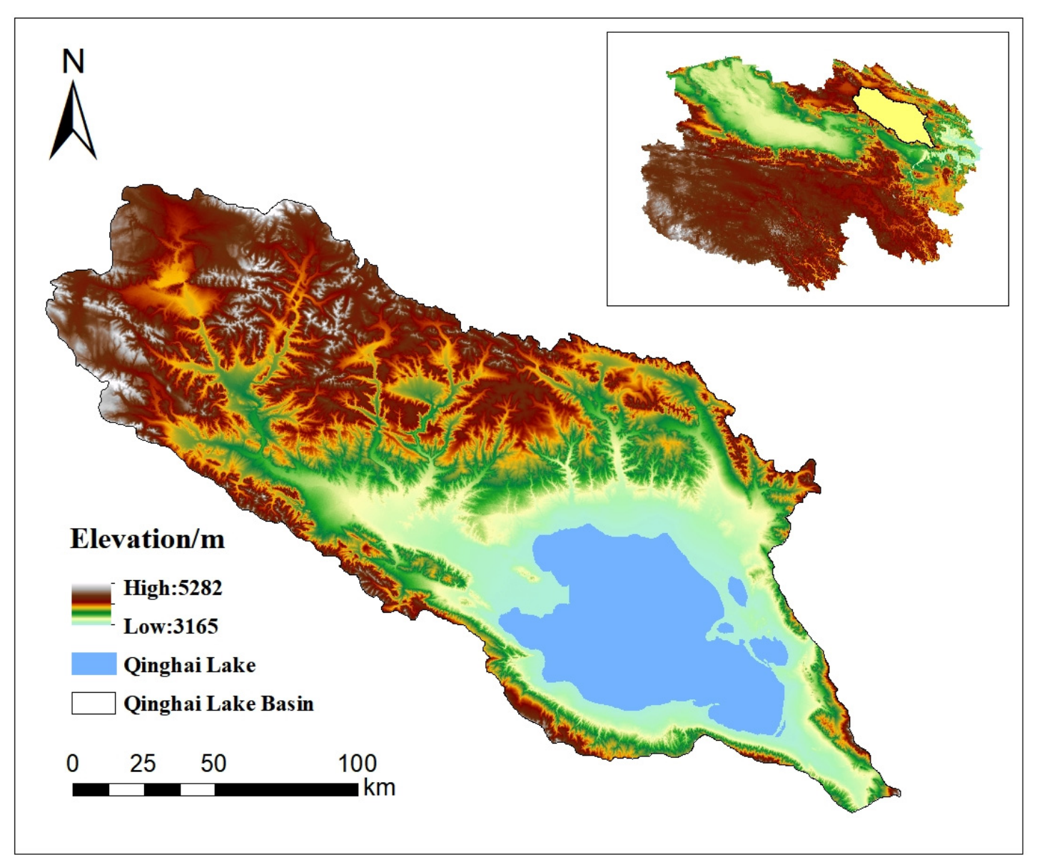
The Qinghai Lake Basin is located in the northeastern Qinghai–Tibet Plateau and encompasses Gangcha County and Haiyan County of Haibei Prefecture, Tianjun County of Haixi Prefecture, and Gonghe County of Hainan Prefecture, covering a total area of 29,661 km², of which the lake surface accounts for approximately 14.7% [23]. The details are shown in Figure 1. The basin lies at the transitional zone between the northwestern arid region, the Loess Plateau, and the alpine region of the Qinghai–Tibet Plateau, and is characterized by a typical semi-arid plateau continental climate. The mean annual temperature ranges from −1.0 °C to 4.0 °C, while the mean annual precipitation varies between 291 mm and 579 mm, with rainfall mainly concentrated in summer, accompanied by abundant sunshine and high evaporation. As a closed plateau inland lake, Qinghai Lake relies primarily on precipitation and snowmelt recharge, which together contribute more than 90% of the total annual runoff. Several major rivers, including the Buha River, Haergai River, Quanji River, and Heima River, flow into the lake. The region’s unique geographical setting has resulted in a fragile ecological base, making it highly sensitive to global climate change and anthropogenic disturbances, and thus susceptible to ecological problems such as SE, grassland degradation, and biodiversity loss. The basin supports a relatively diverse range of ecosystem types, mainly including grassland, wetland, desert, and alpine shrubland [24].

2.2. Data Sources

The datasets employed in this study primarily include elevation, land use, the QLB administrative boundary, mean annual precipitation, soil properties, and vegetation cover, with detailed information regarding data types, sources, spatial resolutions, and temporal coverage summarized in

Table 1. Data sources and descriptions.

Data Type	Data Source	Spatial Resolution	Year
DEM data	Geospatial Data Cloud Platform (https://www.gscloud.cn/) (Accessed: 15 March 2026)	30 m	2010–2023
Land use/land cover data	CLCD China Land Cover Dataset, Wuhan University (http://zenodo.org.cn) (Accessed: 18 March 2026)	30 m	2010–2023
Basin boundary data	National Geographic Information Center (https://www.webmap.cn/) (Accessed: 21 March 2026)	/	/
Precipitation data	National Tibetan Plateau Data Center (https://data.tpdc.ac.cn/) (Accessed: 17 March 2026)	1 km	2010–2023
Soil data	Harmonized World Soil Database (HWSD), FAO (https://gaez.fao.org/pages/hwsd) (Accessed: 2 April 2026)	250 m	2010–2023
Vegetation cover data	NASA (https://ladsweb.modaps.eosdis.nasa.gov/) (Accessed: 25 March 2026)	250 m	2010–2023

. To ensure compliance with the input requirements of the InVEST model concerning the spatial consistency of multi-source raster data, a standardized preprocessing workflow was implemented for all raster datasets. Specifically, the coordinate reference system for all data layers was uniformly transformed to WGS_1984_UTM_Zone_47N. Using the 30 m resolution DEM as the baseline, continuous raster layers were resampled via bilinear interpolation, whereas the land use classification raster was resampled using the nearest neighbor method to preserve categorical integrity. Subsequently, all layers were masked and clipped to the QLB boundary to guarantee uniform spatial extent and consistent pixel size across the entire basin. Finally, a limited number of missing pixels were addressed through neighborhood filling, and invalid pixels outside the basin were excluded, thereby accomplishing the standardization of the multi-source data grid. All preprocessing operations were carried out using ArcGIS 10.8 (Esri, Redlands, CA, USA).

2.3. Methodology

2.3.1. Invest Model

This study focuses on the QLB as the research area and applies the Sediment Delivery Ratio (SDR) module of the InVEST 3.20.0 model to quantitatively evaluate SC. This module, which is rooted in the Universal Soil Loss Equation (USLE), synthesizes a variety of influencing factors—including rainfall erosivity, soil attributes, topographic conditions, vegetation coverage, and soil and water conservation practices [25]—in order to characterize the spatiotemporal evolution of SC and identify its principal driving forces. Such an integrated assessment provides a robust scientific underpinning for regional soil conservation planning and the formulation of ecological restoration strategies. A key advancement of this model over the conventional USLE is its inclusion of the sediment retention functionality of downslope grid cells, thereby overcoming a major limitation of the traditional approach, which disregards the sediment interception effects exerted by downstream terrain and vegetation during transport processes [26].

The modeling exercise comprised independent static simulations for four selected periods—2010, 2015, 2020, and 2023—with no inter-annual iterative coupling between periods. For the computation of flow accumulation, the multiple flow direction (MFD) algorithm was implemented, and the threshold flow accumulation (TFA) was fixed at 1000 pixels to enable the delineation of sub-watershed units across the basin. Furthermore, the piecewise threshold parameters governing the sediment delivery ratio were specified as SDR_max = 0.8, IC₀ = 0.5, and k = 2. The corresponding computational formulas are provided below [27].

$$SEDRET=PKLS-USLE+SEDR$$

$$PKLS=R·K·LS$$

$$USLE=R·K·LS·C·P$$

where SEDRET represents the soil conservation amount, and SEDR denotes the sediment retention amount. PKLS indicates the potential soil loss under prevailing geomorphological and climatic conditions, whereas USLE refers to the actual soil erosion amount, i.e., the soil loss after the modulating effects of vegetation cover and soil and water conservation practices. The factors R, K, LS, C, and P correspond to rainfall erosivity, soil erodibility, topography, vegetation cover, and conservation practices, respectively.

2.3.2. Calculation of Parameters Related to Sc

(1)

Rainfall Erosivity Factor (R)

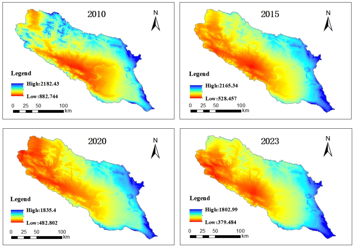
Rainfall erosivity serves as the fundamental dynamic driver of SE triggered by rainfall, reflecting the synergistic effects of rainfall kinetic energy and rainfall intensity. In this study, the rainfall erosivity factor (R) was derived from the annual precipitation datasets of the Qinghai–Tibet Plateau spanning the period 2010–2023, and was computed using the following formula [28], as shown in Figure 2.

$$R=\alpha \times P^{\beta }$$

where R is the mean annual rainfall erosivity, P is the annual precipitation (mm), and α and β are empirical coefficients, set at 0.0534 and 1.6548, respectively.

(2)

Soil Erodibility Factor (K)

Soil erodibility reflects the susceptibility of soils to raindrop impact and runoff scouring, and is primarily governed by soil properties such as particle size distribution, organic matter content, and structural stability. Following the EPIC (Erosion Productivity Impact Calculator) model developed by Williams et al. [29], the K factor was computed using the revised parameters of Zhang Keli et al. [30], which have been calibrated to represent the soil characteristics of most regions across China. The calculation formula is as follows:

$$SNI=1-{\displaystyle \frac{SAN}{100}}$$

$$K=0.1317(0.2+0.3exp(-0.0256SAN(1-SIL/100))){({\displaystyle \frac{SIL}{CLA+SIL}})}^{0.3}$$

$$(1-{\displaystyle \frac{0.25C}{C+exp(3.72-2.95C)}})(1-{\displaystyle \frac{0.7SNI}{SNI+exp(-5.51+22.9SNI)}})$$

where SAN, SIL, and CLA represent the percentages of sand, silt, and clay, respectively, and C denotes the soil organic matter content (%). Since the K value derived from the above equation is expressed in the American customary unit system, a conversion factor of 0.1317 is applied to convert it to the internationally standard unit of t·hm²·MJ⁻¹·mm⁻¹·hm⁻².

(3)

Slope Length and Steepness Factor (Ls)

The LS factor serves as an integrated topographic indicator reflecting the influence of terrain on SC [31]. In this study, the 30 m resolution DEM data of the QLB were preprocessed via sink-filling, after which the slope steepness factor (S) and slope length factor (L) were derived using the estimation method developed by Zhang et al. [32]. The specific algorithms employed were based on the CSLE (Chinese Soil Loss Equation) framework, as adopted in the China Water Conservancy Census [33,34].

$$\mathrm{m}=\left\{\begin{array}{c}\theta \le 0.57° m=0.2\\ 0.57°<\theta \le 1.72° m=0.3\\ 1.72°<\theta \le 2.86° m=0.4\\ 2.86°<\theta m=0.5\end{array}\right.$$

$$L={\left({\displaystyle \frac{\lambda }{22.1}}\right)}^m$$

$$S=\left\{\begin{array}{c}10.80\sin \theta +0.03 \theta \le 5°\\ 16.80\sin \theta -0.50 5°<\theta \le 10° \\ 21.91\sin \theta -0.96 \theta >10°\end{array}\right.$$

where m is the slope gradient exponent, θ is the slope angle (°), L is the slope length factor, λ is the horizontal projection of slope length (m), and S is the slope steepness factor.

(4)

Vegetation Cover and Management Factor (C)

The C factor reflects the influence of land use type and vegetation cover on SC [35]. In this study, the C factor was estimated using the method of Cai Chongfa et al. [36], which is based on fractional vegetation cover and yields values between 0 and 1. A higher C value indicates greater SE severity and, accordingly, a diminished capacity for SC. The specific formula used is as follows:

$$C=\left\{\begin{array}{c}1 f=0\\ 0.6508-0.3436\log \left(f\right) 0<f\le 78.3\%\\ 0 f>78.3\%\end{array}\right.$$

$$f={\displaystyle \frac{NDVI-{NDVI}_{min}}{{NDVI}_{max}-{NDVI}_{min}}}$$

where C is the vegetation cover and management factor, and f is the fractional vegetation cover (FVC, %). NDVI is the pixel-based vegetation index, while NDVI_min and NDVI_max correspond to the vegetation index values for bare soil pixels and fully vegetated pixels, respectively.

(5)

Soil and Water Conservation Practice Factor (P)

The P factor quantifies the effectiveness of soil and water conservation measures—including engineering structures, tillage practices, and vegetative interventions—in mitigating SE, with values spanning from 0 to 1; a more comprehensive suite of control measures corresponds to a lower p value. In this study, p values for different land use categories were assigned based on established methodologies from previous investigations [37,38], as summarized in

Table 2. p values for different land use types.

Land Use Type	Cropland	Forestland	Grassland	Water Body	Snow/Ice	Bare Land
p value	0.4	1	1	0	1	1

. While earlier studies have predominantly concentrated on six fundamental land use classes [18], the Wuhan University CLCD dataset does not include built-up land; consequently, glacier/snow-covered land was incorporated into our analysis. Given that this land cover type is devoid of any soil and water conservation measures, its p value was set to 1, in accordance with Meusburger et al. [39]. The P-factor assignments in the present study were informed by both the prevailing environmental conditions of the QLB and relevant findings from plateau-specific research. Cropland, which occupies a limited spatial extent within the basin and is subject only to rudimentary field-based conservation practices in areas surrounding the lake, was assigned a p value of 0.4. Water bodies were assigned a p value of 0, as these areas are not susceptible to soil erosion processes. Forestland and grassland, which are predominantly characterized by natural alpine vegetation ecosystems with virtually no anthropogenic conservation engineering, together with bare land and glacier/snow-covered terrain—both lacking any conservation interventions—were uniformly assigned a p value of 1. This assignment framework adequately reflects the actual conditions of soil and water conservation measures within the study area. Nevertheless, in the absence of localized field experimental data, the P factor was not subject to local calibration. The potential implications of these assignments for SC estimation outcomes will be critically examined through an uncertainty analysis in the Discussion Section 4.4.

2.3.3. Geodetector Model

The GeoDetector model is a widely used statistical tool in geospatial research for detecting spatial heterogeneity and quantifying the explanatory power of driving factors [40]. This model not only enables the quantitative characterization of individual factor contributions to the dependent variable, but also effectively captures the interaction effects between pairs of factors [41], thus facilitating a deeper understanding of synergistic or antagonistic relationships among drivers. In the present study, the GeoDetector was employed to quantitatively investigate the driving mechanisms underlying the spatial heterogeneity of SC. The q-statistic, which ranges from 0 to 1, was adopted to evaluate the explanatory power of each factor; a q-value approaching 1 indicates stronger explanatory capacity and, consequently, a greater influence on the spatial differentiation of SC [41].

Based on both the established knowledge of primary controlling factors in soil conservation studies conducted in alpine basins and the availability of data, six variables—namely SC, soil type, DEM, slope, FVC, and LUCC—were selected as explanatory factors for the GeoDetector analysis. The discretization intervals for each continuous factor were defined as follows: FVC was classified into six categories: 0–0.15, 0.15–0.33, 0.33–0.54, 0.54–0.72, 0.72–0.88, and 0.88–1; DEM was grouped as <3274 m, 3274–3524 m, 3524–3764 m, 3764–3996 m, 3996–4245 m, and >4245 m; slope was divided into 0–3.2°, 3.2–8.1°, 8.1–14.2°, 14.2–21.1°, 21.1–29.1°, and >29.1°; and soil type was categorized as <7001, 7001–11,182, 11,182–11,425, 11,425–11,568, 11,568–11,765, and 11,765–11,927. It is important to note that the q-values derived from the GeoDetector are somewhat sensitive to the discretization scheme employed. To mitigate this sensitivity, all continuous factors were uniformly categorized into six classes, with class boundaries determined automatically using the natural breaks (Jenks) method, which minimizes within-class variance. The selection of six classes also draws upon the common practice adopted in previous GeoDetector applications in alpine basin contexts [41], thereby ensuring sufficient sample sizes within each class while preserving computational stability. To guarantee the comparability of q-values across different study years, the classification boundaries for each factor were held constant for 2010, 2015, 2020, and 2023.

$$\mathrm{q}=1-{\displaystyle \frac{1}{N{\sigma }^2}}{\displaystyle \sum _{\mathrm{h}=1}^L{N}_{\mathrm{h}}{\sigma }_{\mathrm{h}}^2}$$

where q is the detection power of the driving factors; L is the number of stratified subregions; N denotes the total number of samples across the study area; σ² is the overall variance of the study area; N_h is the number of samples in subregion h; and σ_h² is the variance within subregion h.

3. Results and Analysis

3.1. Spatiotemporal Characteristics of Sc Services in the QLB

3.1.1. Temporal Variation Characteristics

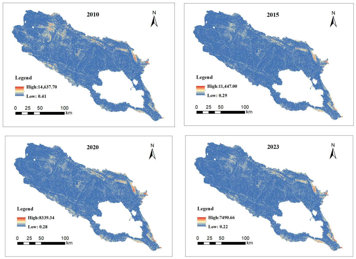
Over the 14-year study period, SC services in the QLB exhibited a progressive declining trend across the selected time points, characterized by a pronounced stage-dependent reduction, with total SC values ranging from 0.22 to 14.64 × 10³ t. The SC potential within high-value zones—representative of areas with elevated functionality—decreased persistently from 14.64 × 10³ t in 2010 to 11.45 × 10³ t in 2015, corresponding to a reduction of approximately 21.79%. This declining trajectory continued, with SC dropping to 8.34 × 10³ t in 2020 and reaching its nadir of 7.49 × 10³ t in 2023, yielding a cumulative decrease of 48.84% over the entire study period and evidencing a clear monotonic decreasing trend. Concurrently, low-value zones experienced a decline from 0.41 × 10³ t to 0.22 × 10³ t, indicating that even the modest SC capacity of low-functionality areas—situated on an ecologically vulnerable substrate—has been steadily eroding. The delineation of high-, medium-, and low-value zones was performed using the natural breaks method on an annual basis. The relative areal proportions of these classes across the basin were approximately 12–15% for high-value zones, 35–40% for medium-value zones, and 45–53% for low-value zones. Notably, the high-value zones occupied the smallest proportion and exhibited a shrinking tendency over the study period, whereas the low-value zones demonstrated continuous areal expansion. Collectively, the peak SC value in the basin was recorded in 2010, with no subsequent recovery observed, thereby reflecting a sustained degradation trend in SC services throughout the investigated timeframe.

3.1.2. Spatial Variation Characteristics

From a spatial perspective (Figure 3), SC in the QLB generally exhibited a pattern of “low in the center and high along the margins,” with relatively elevated values also observed in the northwestern portion of the basin. Over the study period, high-value SC zones remained limited in extent and appeared as fragmented patches, mainly concentrated in forest–grassland transition belts at higher elevations in the northwestern, southeastern, and southwestern parts of the basin, forming a narrow strip oriented northwest–southeast. Medium-value zones were chiefly located in the central area of Tianjun County in the northwest, the central and northern parts of Gangcha County, and along the southwestern boundary. Low-value zones occupied the largest and most contiguous area, consistently distributed across the low-elevation plains surrounding the lake, along riverbanks, and in the bare land and grassland areas of the northwestern corner.

3.2. Effects of Different Land Use Types on Sc Function

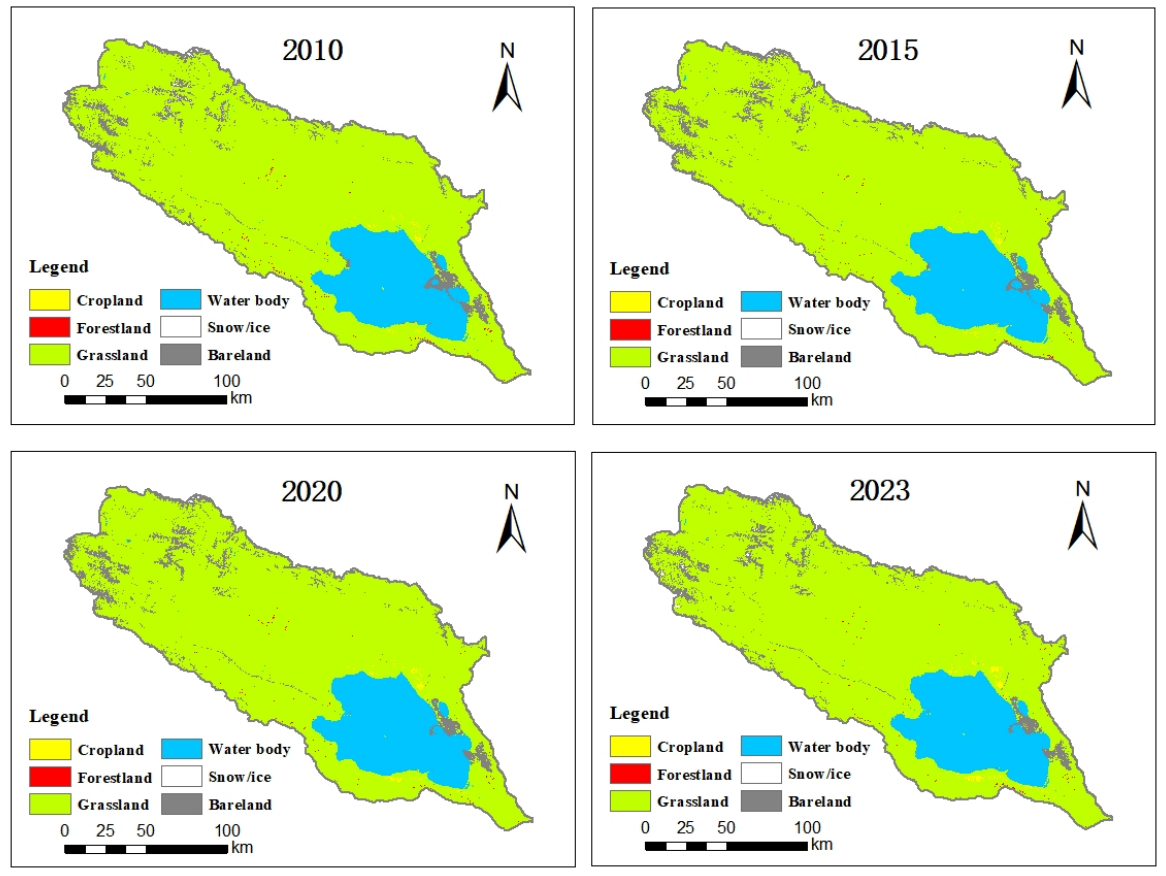
The land use types in the QLB mainly include cropland, forestland, grassland, water bodies, ice and snow cover, and bare land (Figure 4), with marked differences in SC capacity across categories (

Table 3. SC and SE intensities by different land use types (t·hm⁻²·a⁻¹).

	Land Use Type	2010	2015	2020	2023
SC	Cropland	15.82	14.22	12.17	12.90
	Forestland	252.27	213.92	176.67	165.49
	Grassland	111.31	82.74	67.66	61.57
	Bare land	198.39	135.32	103.27	94.51
SE	Cropland	0.00	0.01	0.00	0.01
	Forestland	0.23	0.29	0.59	0.76
	Grassland	1.16	1.23	0.67	0.77
	Bare land	19.13	14.21	9.66	8.93

). From 2010 to 2023, SC amounts for all land use types showed a continuous decreasing trend, with the most notable declines occurring during 2010–2020. By 2020, SC values had generally fallen to their lowest levels over the study period and remained low with slight fluctuations in 2023. Forestland, bare land, and grassland were the predominant contributors to SC, with their SC amounts far exceeding those of cropland and water bodies. Specifically, SC decreased by 34.40% in forestland, 52.36% in bare land, and 44.69% in grassland, indicating a widespread degradation of SC function across these types. Cropland exhibited extremely low SC values with relatively minor reductions, contributing only marginally to overall SC services. SE intensity showed an inverse pattern relative to SC capacity. Although SE intensities for forestland and grassland remained relatively low—ranging from 0.23 to 0.76 t·hm⁻²·a⁻¹ and 0.67 to 1.23 t·hm⁻²·a⁻¹, respectively—they displayed a slight upward trend after 2020, suggesting an increasing erosion risk. Bare land exhibited the highest SE intensity, varying between 8.93 and 19.13 t·hm⁻²·a⁻¹, thus representing the primary erosion source within the basin. Overall, SC services in the basin exhibited a comprehensive declining trend across the selected years, with a pronounced weakening of forest and grassland ecosystem functions and a continuous loss of SC capacity in bare land areas. In the future, it is urgently necessary to implement differentiated soil and water conservation interventions targeting forest–grassland conservation and bare land management, so as to curb the persistent decline in the overall SC function of the basin.

3.3. Vertical Differentiation of Sc Services Across Different Elevation Gradients

SC intensity in the QLB exhibited a statistically significant increasing trend with rising elevation, whereas total SC was predominantly concentrated in the mid-to-high elevation belts, revealing a distinctly asymmetric distribution pattern (

Table 4. SC and SE intensities at different elevations (t·hm⁻²·a⁻¹).

	Elevation	2010	2015	2020	2023
SC	3100~3500	47.61	39.41	33.91	30.80
	3500~4000	123.34	94.34	79.52	70.68
	4000~4500	151.75	106.19	83.07	76.38
	>4500	211.02	134.46	98.96	93.65
SE	3100~3500	0.59	0.67	0.40	0.45
	3500~4000	1.32	1.43	0.82	0.91
	4000~4500	3.29	2.78	1.84	1.75
	>4500	18.52	13.20	8.66	8.07

). In the low-elevation zone (3100–3500 m), despite its considerable areal extent, SC capacity remained relatively constrained, primarily owing to the prevalence of cropland and low-coverage grassland, together with frequent anthropogenic surface disturbances. The 3500–4000 m zone constituted the primary contributing belt for total SC, characterized by extensive high-coverage grassland and shrubland, where root–soil stabilization and favorable slope convergence conditions facilitated effective sediment trapping and deposition, thereby yielding the highest total SC contribution. The 4000–4500 m zone served as the secondary contributing belt, with SC capacity slightly lower than that of the primary belt. In the high-elevation zone (>4500 m), although SC intensity reached its maximum, the reduction rate exceeded 55%, with the rate of attenuation accelerating at higher altitudes—a phenomenon that may be attributable to the heightened sensitivity of these alpine environments to climatic variability. SE intensity also demonstrated an increasing trend with elevation. Notably, in areas above 4500 m, SE intensity declined from 18.52 t·hm⁻²·a⁻¹ to 8.07 t·hm⁻²·a⁻¹, a reduction that may be closely linked to the extensive distribution of alpine bare land, low vegetation cover, and pronounced freeze–thaw activity. The decreasing trend in SE intensity across all elevation gradients over time may be associated with the weakening of regional rainfall erosivity (Figure 3) or localized improvements in surface vegetation cover in recent years. Looking ahead, priority should be given to the conservation of vegetation-covered areas at mid-elevations, alongside the strengthening of dynamic monitoring and adaptive management strategies for the ecologically fragile high-elevation zones, so as to preserve the stability of cascading SC functions across the basin.

3.4. Effects of Different Slope Gradients on Sc Function

In the QLB, total SC was predominantly concentrated within the gentle-to-moderate slope classes (5–25°), whereas SC intensity exhibited a non-linear increasing trend with steepening slopes, thereby revealing a clear mismatched distribution pattern between total SC and intensity peaks (

Table 5. SC and SE intensities by different slope grades (t·hm⁻²·a⁻¹).

	Slope Gradient	2010	2015	2020	2023
SC	0~5°	25.94	20.30	16.32	15.13
	5~15°	105.67	78.91	64.63	58.41
	15~25°	227.83	166.11	135.22	122.43
	25~35°	335.81	238.90	193.34	174.84
	>35°	426.14	291.89	239.46	214.23
SE	0~5°	0.30	0.32	0.18	0.20
	5~15°	1.39	1.38	0.80	0.87
	15~25°	4.19	3.74	2.30	2.36
	25~35°	12.60	10.04	6.97	6.28
	>35°	18.52	14.51	10.38	9.23

). The 5–15° and 15–25° slope classes emerged as the dominant contributing zones, collectively accounting for 62–68% of the basin’s total SC—a proportion substantially exceeding that of all other slope categories. In the gentle slope zone (0–5°), despite its considerable areal extent, both total SC and intensity remained at their lowest levels, primarily due to limited runoff sediment transport capacity. Conversely, the extremely steep slope zone (>35°) exhibited the highest SC intensity per unit area; however, owing to its negligible areal proportion (less than 5%) and steep topography, its contribution to total SC remained comparatively modest, accounting for only 6–9%. With respect to SC intensity, the >35° zone demonstrated the highest erosion resistance intensity, which declined from 426.14 t·hm⁻²·a⁻¹ in 2010 to 214.23 t·hm⁻²·a⁻¹ in 2023, corresponding to a reduction of 49.73%, followed by the 25–35° and 15–25° gradients. Across all slope classes, SC intensity exhibited a sustained declining trend after peaking in 2010. The observed enhancement of SC capacity on slopes may be attributed to the combined effects of increased runoff sediment transport and deposition processes, as well as the synergistic influences of root –soil stabilization and enhanced surface roughness on steeper terrain. SE intensity also increased with slope steepness, with the >35° zone exhibiting the highest erosion risk, decreasing from 18.52 t·hm⁻²·a⁻¹ to 9.23 t·hm⁻²·a⁻¹ over the study period. In future management efforts, priority should be assigned to vegetation conservation and tillage management in the gentle-to-moderate slope zones (5–25°), while simultaneously strengthening soil erosion control measures in the extremely steep slope zones (>35°), so as to sustain the overall stability of SC functions at the hillslope scale within the basin.

3.5. Analysis of Spatial Heterogeneity in Sc Services

3.5.1. Single-Factor Analysis of Spatial Differentiation

To gain a deeper understanding of the spatial heterogeneity of SC in the QLB, the GeoDetector model was employed to quantitatively evaluate the primary driving factors (

Table 6. Results of single-factor detection.

Year	X1		X2		X3		X4		X5
	q	p	q	p	q	p	q	p	q	p
2010	0.096	0.000	0.166	0.000	0.774	0.000	0.035	0.000	0.048	0.000
2015	0.069	0.000	0.113	0.000	0.659	0.000	0.013	0.000	0.032	0.000
2020	0.065	0.000	0.099	0.000	0.682	0.000	0.020	0.000	0.023	0.000
2023	0.064	0.000	0.098	0.000	0.650	0.000	0.017	0.000	0.024	0.000

Note: X1, soil type; X2, elevation; X3, slope; X4, vegetation cover; X5, land use.

). The results demonstrated that all selected factors exhibited p-values below 0.001, indicating that their explanatory power with respect to SC spatial differentiation was statistically significant at an extremely high confidence level. The single-factor contribution rates, as measured by the q-statistic, were ranked in the following descending order: slope (X3) > elevation (X2) > soil type (X1) > land use (X5) > vegetation cover (X4). Specifically, slope (X3) emerged as the factor exerting the strongest explanatory power over SC spatial heterogeneity, with q-values ranging from 0.650 to 0.774—substantially higher than those of the other factors. Elevation (X2) ranked second, with q-values between 0.098 and 0.166, demonstrating a moderately low yet relatively stable explanatory capacity over time. Soil type (X1) yielded q-values ranging from 0.064 to 0.096; its comparatively limited explanatory power may be attributable to the inherent stability of soil properties over short temporal scales. Land use (X5) and vegetation cover (X4) exhibited the lowest explanatory power, with q-values ranging from 0.023 to 0.048 and 0.013 to 0.035, respectively. Collectively, the single-factor detection results reflect that, within the model simulation framework, topographic factors exerted considerably stronger explanatory power over SC spatial heterogeneity than land surface cover factors.

3.5.2. Interaction Factor Analysis of Spatial Differentiation

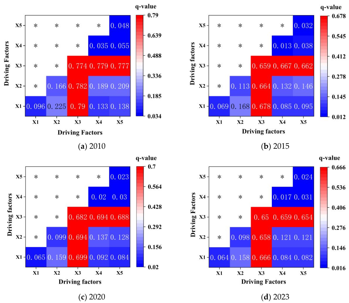
To elucidate the effects of multi-factor synergistic interactions on SC, interaction detection among driving factors was conducted across the study period (Figure 5). The results revealed that the q-values of all pairwise factor interactions were significantly higher than those of individual factors, exhibiting either nonlinear or bilinear enhancement patterns. This finding indicates the presence of synergistic amplification effects among factors, whereby the combined explanatory power of multiple factors substantially exceeded that of any single factor. Among the interaction contributions affecting SC in the QLB, the interactions of slope (X3) ∩ soil type (X1) and slope (X3) ∩ vegetation cover (X4) were the most prominent, with q-values ranging from 0.659 to 0.790, thereby constituting the primary interactive combinations. This reflects that the differences in vegetation cover type and land use patterns in steep slope areas exert a high degree of synergistic explanatory power over the model-simulated SC patterns. The interaction of elevation (X2) ∩ slope (X3) ranked second, with q-values ranging from 0.658 to 0.782, suggesting that the coupling of elevation and slope plays an important regulatory role in the vertical differentiation of SC. The interaction of soil type (X1) ∩ vegetation cover (X4) exhibited relatively lower explanatory power, with q-values ranging from 0.084 to 0.133; nevertheless, it remained higher than that of soil type alone, indicating that the synergistic effect of soil properties and surface cover exerts a certain reinforcing influence on local SC. From a temporal perspective, the q-values of slope consistently remained above 0.65 across all years, underscoring that slope served as the core factor within the synergistic interaction framework.

In summary, the spatial heterogeneity of model-simulated SC in the QLB was most strongly explained by slope-related interactive combinations, with slope (X3) ∩ soil type (X1) and slope (X3) ∩ vegetation cover (X4) identified as the core interactive combinations. In future research, greater attention should be paid to the driving effects of multi-factor coupling mechanisms in SC service degradation, with particular emphasis on the synergistic regulation of extremely steep slopes and high-elevation transition zones.

4. Discussion

4.1. Spatiotemporal Characteristics of Sc Change

This study revealed that SC in the QLB exhibited a pronounced declining trend across the selected years from 2010 to 2023, decreasing from 14.64 × 10³ t to 7.49 × 10³ t, corresponding to a cumulative reduction of 48.84%. This trajectory is broadly consistent with the findings of Shi et al. [18] regarding SC services in the QLB. Spatially, high-value areas were predominantly concentrated in the high-altitude forest–grassland ecotones situated in the northwestern, southeastern, and southwestern sectors of the basin, whereas low-value areas were mainly distributed in the low-altitude flat zones surrounding the lake—a pattern that aligns with the spatial differentiation of habitat quality reported by Han et al. [5]. Along the elevational gradient, the mid-to-high elevation zones (3500–4500 m) contributed the most to total SC, while the high-elevation zone (>4500 m) exhibited a marked reduction of 55.62%, a phenomenon potentially attributable to permafrost degradation and diminished vegetation productivity in high-altitude regions under a warming climate. With respect to slope differentiation, total SC was predominantly concentrated in the gentle-to-moderate slope zones (5–25°), with SC intensity increasing non-linearly with steepening slopes—a finding that corroborates the conclusions of Zhang et al. [42]. In comparison with other alpine and endorheic lake basins on the Qinghai–Tibet Plateau, the declining SC trend identified in this study conforms to the general pattern of climate warming-induced degradation of alpine ecological services. However, the relatively substantial magnitude of SC loss observed in the QLB is closely associated with long-term grazing disturbances and the semi-arid environmental context, with the marginal forest–grassland ecotones serving as SC hotspots that further underscore the region’s distinctive ecological characteristics.

4.2. Synergistic Mechanisms of Driving Factors

The GeoDetector results indicated that slope was the factor exerting the strongest explanatory power over the spatial heterogeneity of model-simulated SC, followed by elevation, whereas land use and vegetation cover exhibited comparatively lower explanatory capacity. Over the study period, the q-values of slope ranged from 0.650 to 0.774, displaying notable interannual fluctuations that were primarily modulated by year-to-year variations in rainfall, which in turn influence slope runoff erosion intensity. The q-values of elevation ranged from 0.098 to 0.166, with relatively moderate interannual variability; their fluctuations may be indirectly attributable to interannual changes in high-altitude vegetation distribution and freeze–thaw activity. This finding diverges from the results of Cao et al. [43], who identified elevation as the core factor influencing water yield services, reflecting the fact that different ecosystem services are governed by distinct controlling factors—soil conservation is more directly regulated by topographic factors, whereas water yield services are primarily controlled by precipitation and evapotranspiration. Interaction detection further revealed that slope ∩ soil type and slope ∩ vegetation cover constituted the core interactive combinations, reflecting the synergistic regulatory effect of the “topography–soil–vegetation” coupled system on SC—a finding consistent with the observations of Jiang et al. [3] in the Three Gorges Reservoir area. However, it is important to note that the dependent variable (SC) was simulated by the InVEST model, and slope, soil type, FVC, and LUCC all participate in the SC calculation through their respective parameters (LS, K, C, and P), thereby giving rise to an inherent structural dependency between the explanatory variables and the response variable. Consequently, the q-values reflect the explanatory power of each factor with respect to the spatial heterogeneity of model-output SC, rather than constituting independent causal evidence.

4.3. Differentiated Responses of Sc Function Across Land Use Types

Forestland, bare land, and grassland emerged as the dominant contributing land use types, exhibiting a degradation sequence of bare land > grassland > forestland. Notably, despite the implementation of various ecological engineering initiatives in the QLB since the beginning of this century—including the Grain-for-Green Program, the Three-River-Source Ecological Protection Project [44,45], and grassland grazing bans alongside livestock–grassland balance policies [46]—SC did not exhibit a recovery trend over the study period. This phenomenon is attributable to the combined effects of multiple superimposed factors; however, constrained by the current data availability and methodological limitations, this study is unable to rigorously quantify the individual contributions of these factors. First, the positive effects of vegetation restoration on SC may be subject to time-lag effects, with response delays potentially extending to 5–10 years or more under alpine environmental conditions. Second, the continuous rise in QLB water levels [21] has progressively expanded the lakeshore inundation zone, which may have altered the hydrological regime and erosion patterns in the lake-surrounding areas. Third, climate warming has intensified permafrost degradation at high elevations, thereby increasing the supply of loose slope materials and partially offsetting the soil-stabilizing benefits conferred by vegetation. Overall, the contributions of the above factors to the absence of SC recovery are likely synergistic and overlapping in nature. However, given that the InVEST-SDR model is not designed as a tool for disentangling multi-factor contributions, and that existing monitoring data are insufficient to support independent validation of each factor, this study is presently unable to quantitatively distinguish their respective relative contribution rates. This important issue should be prioritized as a key direction for future research.

4.4. Limitations and Future Directions

This study is subject to several limitations that should be acknowledged. First, socioeconomic factors—including population growth, grazing intensity, and ecological compensation policies—were not incorporated into the analytical framework assessing their potential impacts on SC. Second, the temporal coverage of the dataset is relatively limited, and future multi-scenario simulations were not conducted. Third, owing to the absence of field-measured soil erosion and sediment transport data, independent validation of the InVEST-SDR model was not feasible. Consequently, the key parameters—namely K, LS, C, and P—were assigned based on empirical formulas and literature-derived values, without local calibration. Such parameterization uncertainties may introduce systematic overestimation or underestimation of the absolute magnitudes of SC and SE. Fourth, the resampling of multi-source datasets to a uniform 30 m resolution may exert a minor influence on local-scale visualization details; however, this does not compromise the macroscopic spatial differentiation patterns or the ranking of factor importance. It is important to emphasize that the systematic biases inherent in the above parameter assignments have relatively limited influence on the spatial configuration of SC, the relative trends across land use types, elevation gradients, and slope classes, or the factor priority order identified by the GeoDetector. Therefore, the present study primarily focuses on the analysis of spatiotemporal differentiation patterns and the coupling relationships among driving factors. The absolute values derived from the model outputs should not be directly applied to precise engineering calculations. Nevertheless, the core conclusions—including the persistent degradation trend of SC, the slope-dominated factor ranking, and the identification of core interactive combinations—are grounded in relative comparative analysis, and are thus scientifically robust and reliable. Future research should prioritize the local calibration of model parameters using field-measured data, and integrate FLUS (developed by the School of Geography and Planning, Sun Yat-sen University, Guangzhou, China)/CLUE-S (developed by Wageningen University, Wageningen, The Netherlands) models with climate change scenarios to conduct scenario-based simulations of SC functions in the lakeshore zone under the context of continuously rising QLB water levels, thereby further enhancing the accuracy and applicability of the results.

5. Conclusions

(1) From 2010 to 2023, SC services in the QLB exhibited a progressive declining trend across the selected study years. The total SC within high-value zones decreased from 14.64 × 10³ t to 7.49 × 10³ t, corresponding to a cumulative reduction of 48.84%, while that within low-value zones declined from 0.41 × 10³ t to 0.22 × 10³ t. Spatially, high-value areas were predominantly concentrated in the high-altitude forest–grassland ecotones located in the northwestern, southeastern, and southwestern portions of the basin, displaying a narrow, elongated distribution aligned along a northwest–southeast axis. In contrast, low-value areas were continuously distributed across the low-altitude zones surrounding the lake, along riverbanks, and in the northwestern corner of the basin.

(2) SC capacity varied considerably among different land use types, with forestland, bare land, and grassland emerging as the dominant contributing categories. Bare land exhibited the highest SE intensity, ranging from 8.93 to 19.13 t·hm⁻²·a⁻¹, thereby functioning as the primary erosion source area within the basin. Notably, SE intensity in forestland and grassland displayed a slight increasing trend after 2020. Along the elevational gradient, total SC was predominantly contributed by the mid-to-high elevation zones (3500–4500 m), with SC intensity increasing progressively with rising elevation. With respect to slope classes, total SC was mainly concentrated in the gentle-to-moderate slope zones (5–25°), whereas SC intensity exhibited a non-linear increase with steeper slopes. The extremely steep slope zone (>35°) exhibited the highest SC intensity; however, owing to its limited areal proportion, its contribution to total SC remained relatively constrained.

(3) The GeoDetector results indicated that slope was the single factor exerting the strongest explanatory power over the spatial heterogeneity of model-simulated SC, followed by elevation, whereas vegetation cover and land use exhibited comparatively lower explanatory capacity. Interaction detection further revealed that all pairwise factor interactions exhibited either nonlinear or bilinear enhancement, with slope ∩ soil type and slope ∩ vegetation cover identified as the primary interactive combinations. This finding reflects the synergistic regulatory effect of the “topography–soil–vegetation” coupled system on SC function.

As an important ecological barrier in the northeastern Qinghai–Tibet Plateau, the continued degradation of SC functions in the QLB poses a direct and imminent threat to regional ecological security. Based on the model simulation results, it is recommended that priority attention be given to the following areas: (1) the mid-to-high elevation zones (3500–4500 m), which serve as the primary contributors to total SC, where vegetation conservation and grazing management should be reinforced; (2) the gentle-to-moderate slope zones (5–25°), which represent the main contributing belt for total SC, where tillage practices and vegetation cover maintenance should be optimized; and (3) the extremely steep slope zones (>35°), which exhibit the highest SE intensity, where soil erosion prevention and control measures should be prioritized. It should be noted that these recommendations are subject to the limitations arising from the lack of local calibration of model parameters, and should therefore be further validated with field-measured data prior to implementation. Meanwhile, future efforts should strengthen the tracking and evaluation of the effectiveness of ecological engineering interventions, as well as the localized determination of model parameters, so as to provide a more robust scientific basis for ecological restoration and sustainable development in the basin.

References

1. Wei, H.; Ma, Y.; Wang, Y.; Ji, W.; Guo, S.; Cai, E.; Huang, J.; Dong, X.; Li, L. Differential Effects of Mountain–Oasis–Desert Landscape Ecosystem Services on Rural Residents’ Subjective Well-Being. Acta Ecol. Sin. 2026, 46, 6898–6913. [Google Scholar]
2. Ma, A.; Liu, Z.; Sun, Y.; Qin, Y.; He, H.; Li, J.; Yang, H. Ecological Security Network Construction and Multi-Scenario Simulation Analysis in the Ili River Valley. China Environ. Sci. 2026, 1–13. [Google Scholar]
3. Jiang, Y.; Shi, D.; Liu, F.; Xu, Y.; Qiao, J. Spatiotemporal Evolution Characteristics and Driving Forces of Soil Conservation Function in Typical Counties of the Three Gorges Reservoir Area. J. Soil Water Conserv. 2026, 40, 454–464. [Google Scholar]
4. Ding, J.; Zhang, F.; Zhang, Y.; Ning, Y.; Zeng, P. Spatiotemporal Variation of Water Yield in the Qinghai Lake Basin under Climate and Land Use Change. J. Lanzhou Univ. Nat. Sci. 2022, 58, 47–56. [Google Scholar]
5. Han, Y.; Chen, K.; Yu, D. Effects of Land Use Change on Habitat Quality in the Qinghai Lake Basin. Ecol. Environ. Sci. 2019, 28, 2035–2044. [Google Scholar]
6. Zhang, B.; Wang, Z.; Song, F.; Fang, H.; Ma, M.; Zhang, F.; Wu, S.; Feng, H. Assessment of Composite Soil Erosion Intensity and Its Response to Climate Change in the Source Region of the Yellow River under Ecological Restoration. J. Soil Water Conserv. 2026, 40, 311–344. [Google Scholar]
7. Jin, C.; Ma, J.; Zheng, H.; Li, R.; Yang, Y.; Ying, L. Spatiotemporal Changes and Driving Factors of Soil Conservation Services in the Heihe River Basin. Res. Environ. Sci. 2026, 1–14. [Google Scholar]
8. Zheng, Q.; Li, Y.; Su, Z.; Zheng, Y.; Wang, Y. Acid Deposition Exacerbates the Impact of Land Use Change on Spatiotemporal Heterogeneity of Soil Conservation in the Chongqing Section of the Three Gorges Reservoir Area. Sci. Silvae Sin. 2026, 62, 40–53. [Google Scholar]
9. Zhang, J.; Cui, J. Spatiotemporal Changes of Ecosystem Services and Their Multi-Scale Trade-Offs and Synergies in the Black Soil Region of Northeast China under Future Climate Scenarios: A Case Study of Heilongjiang Province. Environ. Sci. 2026, 1–21. [Google Scholar]
10. Dong, J.; Yang, J.; Hao, Y.; Hu, P.; Li, B. Factor Analysis Affecting Water Yield, Soil Conservation, and Their Trade-Offs and Synergies in the Weihe River Basin. Res. Soil Water Conserv. 2026, 33, 189–199, 208. [Google Scholar]
11. Li, T.; Zhu, R.; Li, X.; Kang, J.; Shan, J.; Li, R.; Yin, Z. Soil Conservation in the Zuli River Basin Based on the InVEST Model. J. Desert Res. 2025, 45, 312–322. [Google Scholar]
12. Zhang, X.; Yu, H.; Qi, Y. Spatial Evolution and Driving Factors of Ecosystem Service Value: A Case Study of the Wuling Mountain Area. Ecol. Econ. 2026, 42, 198–210. [Google Scholar]
13. Zhao, Y.; Zhou, J.; Lei, L.; Xiang, J.; Huang, M.; Feng, W.; Zhu, G.; Wei, W.; Wang, J. Identification of Driving Factors of Water Yield in the Upper Reaches of the Shiyang River Based on the InVEST Model. Chin. J. Ecol. 2019, 38, 3789–3799. [Google Scholar]
14. Kou, X.; Li, Q.; Song, Z.; Yu, Q.; Niu, B.; Wang, S.; Mu, K.; Du, W. Spatiotemporal Evolution and Driving Factors of Soil Erosion Function in a Typical Basin of the Alpine Region in the Upper Yellow River. Front. Plant Sci. 2025, 16, 1589848. [Google Scholar] [CrossRef] [Scilit] [PubMed]
15. Yan, X. Spatiotemporal Evolution and Optimal Management of Ecosystem Services in Qinghai Province Based on Supply–Demand Perspective. Master’s Thesis, Qinghai Normal University, Xining, China, 2025. [Google Scholar]
16. Ma, X. Evolution of Ecosystem Service Trade-Offs/Synergies and Supply–Demand Patterns in Qinghai Province. Master’s Thesis, Qinghai Normal University, Xining, China, 2024. [Google Scholar]
17. Chen, Z.; Gao, X.; Liu, Z.; Chen, K. Spatiotemporal Variation of Soil Erosion Characteristics in the Qinghai Lake Basin Based on the InVEST Model. Int. J. Environ. Res. Public Health 2023, 20, 4728. [Google Scholar] [CrossRef] [Scilit] [PubMed]
18. Shi, J.; Zhong, J.; Ma, Y.; Mi, W. Simulation of Soil Conservation Service Function and Driving Factor Analysis in the Qinghai Lake Basin. Resour. Environ. Yangtze Basin 2024, 33, 1286–1297. [Google Scholar]
19. Zhang, J.; Cao, S.; Cao, G.; Chen, K.; Jiang, G.; Zhang, T.; Han, G.; Lin, Y. Dynamic Changes of Soil Conservation in the Qinghai Lake Basin. Bull. Soil Water Conserv. 2016, 36, 326–331, 350. [Google Scholar]
20. Ma, J. Response of Ecosystem Services to Landscape Pattern Changes on the Qinghai–Tibet Plateau: A Case Study of Eastern Qinghai Province. Doctoral Dissertation, Chang’an University, Xi’an, China, 2023. [Google Scholar]
21. Yang, X.M.; Ma, R.C.; Wang, A.M. Impacts of Rising Water Levels in Qinghai Lake on the Socio-Economic Development of the Lake-Surrounding Areas under Climate Warming and Humidification. J. China West Norm. Univ. Nat. Sci. Ed. 2026, 47, 330–336. [Google Scholar]
22. Zhang, Q.; Wang, F.; Li, D.L. Climate Evolution Characteristics and Ecological Effects of the Qinghai Lake Basin under the Intensified Warming and Humidification of the Qinghai–Tibet Plateau. Acta Geogr. Sin. 2024, 79, 1685–1702. [Google Scholar]
23. Li, H.; Li, R.; Yan, X.; Wu, F.; Gao, Z.; Tan, Y. Ecological Risk Assessment and Ecological Function Zoning in the Qinghai Lake Basin. Ecol. Environ. Sci. 2023, 32, 1185–1195. [Google Scholar]
24. Li, D.; Jiang, Z.; Wang, Z. Spatial Characteristics of Biodiversity and GAP Analysis in the Qinghai Lake Area. J. Nat. Resour. 1999, 48–55. [Google Scholar]
25. Li, J.; Liu, L.; Yuan, W.; Luo, Q. Spatial Differentiation Characteristics of Soil Erosion in Central Yunnan Based on the RUSLE Model. J. Southwest Univ. Nat. Sci. Ed. 2026, 46, 140–147. [Google Scholar]
26. Li, M.; He, H.; Wu, D.; Yu, H.; Zhao, L.; Liu, C.; Li, Q.; Hu, Z. Spatiotemporal Evolution of Soil Erosion on the Loess Plateau under Climate Change. Acta Ecol. Sin. 2025, 45, 7793–7807. [Google Scholar]
27. Xie, Y. Spatiotemporal Changes of Ecosystem Services in the Bailongjiang Basin, Gansu, Based on the InVEST Model. Ph.D. Thesis, Lanzhou University, Lanzhou, China, 2015. [Google Scholar]
28. Zhang, R.; Wang, Z.; Ning, Y.; Lou, Y. Spatiotemporal Changes and Driving Mechanisms of Soil Erosion in Hunan Province from 1990 to 2020. Sci. Soil Water Conserv. 2026, 24, 71–85. [Google Scholar]
29. Williams, J.R. The Erosion-Productivity Impact Calculator (EPIC) Model: A Case History. Philos. Trans. R. Soc. B 1990, 329, 421–428. [Google Scholar] [CrossRef] [Scilit]
30. Zhang, K.; Peng, W.; Yang, H. Soil Erodibility and Its Estimation in China. Acta Pedol. Sin. 2007, 44, 7–13. [Google Scholar]
31. Hu, Z.; Liu, X.; Wang, Z.; Li, X.; Wang, W.; Liu, Y. Simulation of Slope Runoff and Sediment Processes Based on Coupled SCS-CN and RUSLE Models: A Case Study of Artificial Rainfall at the Hetonggou Experimental Site. Water Resour. Hydropower Technol. 2026, 1–18. [Google Scholar]
32. Zhang, H.; Wei, J.; Yang, Q.; Baartman, J.; Gai, L.; Yang, X.; Li, S.; Yu, J.; Ritsema, C.; Geissen, V. An Improved Method for Calculating Slope Length (λ) and the LS Parameters of the Revised Universal Soil Loss Equation for Large Watersheds. Geoderma 2017, 308, 36–45. [Google Scholar] [CrossRef] [Scilit]
33. Liu, B.Y.; Nearing, M.A.; Risse, L.M. Slope Gradient Effects on Soil Loss for Steep Slopes. Trans. ASAE 1994, 37, 1835. [Google Scholar] [CrossRef] [Scilit]
34. Liu, B.; Nearing, M.; Shi, P.; Jia, Z. Slope Length Effects on Soil Loss for Steep Slopes. Soil Sci. Soc. Am. J. 2000, 64, 1759. [Google Scholar] [CrossRef] [Scilit]
35. Duan, W.; Han, Y.; Yang, Y.; Wang, Y.; Zhan, X. Impact of Land Use Change on Soil Erosion Intensity in the Baiyangdian Basin. Res. Soil Water Conserv. 2026, 33, 22–31. [Google Scholar]
36. Cai, C.; Ding, S.; Shi, Z.; Huang, L.; Zhang, G. Study on Predicting Soil Erosion in Small Watersheds Using the USLE Model and GIS IDRISI. J. Soil Water Conserv. 2000, 19–24. [Google Scholar]
37. Lu, J.; Chen, X.; Li, H.; Liu, H.; Xiao, J.; Yin, J. Soil Erosion Changes in the Poyang Lake Basin Based on GIS/RS and USLE. Trans. Chin. Soc. Agric. Eng. 2011, 27, 337–344, 397. [Google Scholar]
38. Chen, H.; Ding, W.G.; Zafar, T.B. Evaluation of Soil Water Erosion in Qilian Mountains National Park Based on the USLE Model. Soil Water Conserv. China 2020, 18, 38–44. [Google Scholar]
39. Meusburger, K.; Leitinger, G.; Mabit, L.; Mueller, M.H.; Walter, A.; Alewell, C. Soil Erosion by Snow Gliding—A First Quantification Attempt in a Subalpine Area in Switzerland. Hydrol. Earth Syst. Sci. 2014, 18, 3763–3775. [Google Scholar] [CrossRef] [Scilit]
40. Huang, M.; Yue, W.; Fang, B.; Feng, S. Scale Response Characteristics and Geographic Detection Mechanisms of Ecological Service Value in the Dabie Mountains from 1970 to 2015. Acta Geogr. Sin. 2019, 74, 1904–1920. [Google Scholar]
41. Wang, J.; Xu, C. Geodetector: Principle and Prospective. Acta Geogr. Sin. 2017, 72, 116–134. [Google Scholar]
42. Zhang, J.; Wu, X.; Jiang, Y.; Hua, C.; Song, K.; Cheng, Y. Soil Erosion Assessment in the Heihe River Basin Based on the RUSLE Model. Hubei Agric. Sci. 2026, 65, 31–35. [Google Scholar]
43. Cao, M.; Han, Y.; Liu, Z.; Ma, Y.; Zhao, H.; Chen, C.; Zhu, S.; Chen, K. Spatio-Temporal Evolution and Correlation Analysis of Water Yield and Carbon Storage in the Qinghai Lake Basin. Sustainability 2026, 18, 5569. [Google Scholar] [CrossRef] [Scilit]
44. Xie, L. The Master Plan for Ecological Protection and Construction of the Sanjiangyuan Nature Reserve Enters the Implementation Phase: Li Jincheng Attends the Inauguration Ceremony; Qinghai Daily: Xining, China, 2005; p. 002. [Google Scholar]
45. General Office of the People’s Government of Qinghai Province. Notice on the Establishment of the Project Office for Comprehensive Ecological Protection and Management of the Qinghai Lake Basin; Qinghai Government Gazette: Xining, China, 2008; p. 14.
46. General Office of the People’s Government of Qinghai Province. Notice on Issuing the Implementation Plan for the Third Round of Grassland Ecological Protection Subsidy and Reward Policies in Qinghai Province (2021–2025); Gazette of the People’s Government of Qinghai Province (Chinese Edition): Xining, China, 2022; pp. 3–13.
Figure 1. Location and overview of the study area.
Sustainability 18 09163 g001
Figure 2. Distribution of rainfall erosivity in the QLB from 2010 to 2023.
Sustainability 18 09163 g002
Figure 3. Spatial distribution of SC in the QLB from 2010 to 2023.
Sustainability 18 09163 g003
Figure 4. Distribution of land use types in the QLB from 2010 to 2023.
Sustainability 18 09163 g004
Figure 5. Results of interaction factor detection. Note: “*” indicates nonlinear enhancement, meaning the q-value of the interaction between two factors is greater than the sum of the q-values of the two individual factors.
Sustainability 18 09163 g005