Optimizing Territorial Functional Layouts for Carbon–Economic Coordination Using a Cellular-Automata-Based Multi-Objective Spatially Explicit Model

Abstract

Territorial spatial function layout optimization can alleviate the conflict between low-carbon development and economic growth by regulating the quantitative composition and spatial allocation of production, living, and ecological functions. However, existing spatial optimization models remain limited in their ability to simultaneously address quantitative uncertainty, spatial functional conflicts, and the coordination among spatial layouts, quantitative structures, and optimization objectives. This study develops a cellular automata (CA)-based Territorial Spatial Function Layout Optimization (TSFLO) model. The model integrates multi-objective fuzzy linear programming to optimize the target-year quantitative structure, a non-homogeneous Markov process to characterize functional transitions, and a game-theoretic approach to coordinate spatial conflicts. Furthermore, the model inversely derives the optimal quantitative structure of the base year through the Markov state transition equation, adjusts the base-year layout according to coordinated suitability to construct the CA initial state, and compares the TSFLO model with the PLUS model using Qionglai City, China, as a case study. Relative to the 2020 baseline layout, the proportions of areas without functional transitions under the TSFLO scenario were 81.40% and 73.60% in 2025 and 2030, respectively, which were 3.39 and 0.28 percentage points higher than those of the PLUS model. The maximum absolute relative errors between the TSFLO-optimized results and the target quantitative structure were 0.07% and 0.05%, respectively, representing reductions of 99.28% and 98.52% compared with the PLUS model. The minimum matching degrees between the seven territorial spatial functions and their corresponding high-coordinated-suitability areas were 71.86% and 69.51% in 2025 and 2030, respectively. From 2020 to 2030, the decoupling index of ecological regulation service functions was −2.8642, compared with −1.9128 for PLUS, indicating that the TSFLO scenario improved the decoupling intensity by 49.7%. The results demonstrate that TSFLO can integrate quantity optimization, spatial conflict coordination, and initial state construction within a unified CA framework, thereby improving quantitative allocation accuracy and spatial suitability matching. This provides methodological support for coordinating low-carbon development and economic growth through territorial spatial function layout optimization.

1. Introduction

Excessive carbon emissions causing global warming have become a major international concern [1]. The continued intensification of phenomena such as rising temperatures and glacier retreat poses a severe threat to global ecological security and the sustainable development of the economy [1,2,3]. Carbon emission reduction has become an international consensus. This need is also reflected in international policy agendas. The Sixth Assessment Report of the Intergovernmental Panel on Climate Change (IPCC) identifies spatial planning, urban form, and infrastructure as important strategies for urban emission reduction [4]. The Kunming–Montreal Global Biodiversity Framework (GBF) Target 1 calls for integrated and biodiversity-inclusive spatial planning to address land-use change [5]. Therefore, how to coordinate emission reduction, ecological conservation, and economic development through spatial layout optimization has become a globally relevant planning challenge. However, the economic structures of developing countries, which rely on high-carbon industries, make carbon emission reduction prone to causing economic downturns [6], and it is therefore urgent to explore pathways that achieve synergy between low-carbon and economic growth. Studies have shown that there is a spatial coupling effect between the territorial spatial functional layout (TSFL) and carbon emissions, and that optimizing the spatial layout can effectively reduce carbon emission intensity [7]. For example, China has curbed urban sprawl by demarcating boundaries for urban development, ecological protection, and farmland protection, thereby reducing carbon emission intensity while maintaining economic growth [8]. Therefore, optimizing the TSFL and promoting industrial reforms are important paths for carbon emission reduction while maintaining economic growth and responding to global climate change.

Cellular automata (CA), the conversion of land use and its effects (CLUE-S), and the patch-generating land use simulation (PLUS) models are widely used tools for spatially explicit simulation and allocation [9,10]. CLUE-S allocates land use based on externally defined land-use demands and location suitability [10]. PLUS simulates land-use dynamics through land expansion analysis and patch generation mechanisms, and can be coupled with external quantity optimization models to derive target demands [9,11]. These models establish links between quantitative demands and spatial allocation; however, this does not necessarily indicate that uncertainties in key input parameters have been fully incorporated into the spatial allocation process. Many existing spatial optimization models have not sufficiently considered the impacts of key parameter uncertainties on spatial configurations [12]. In addition, existing models still have varying limitations in coordinating competing functional conflicts and integrating target quantitative structures, CA initial states, and subsequent spatial allocation processes [13,14,15,16]. Therefore, further efforts are needed to integrate uncertainty-aware quantitative optimization, spatial conflict coordination, and initial state construction within a CA framework.

The goal of this study is to develop a territorial spatial function layout optimization (TSFLO) model based on the cellular automata (CA) framework, aiming to achieve the coordinated optimization of spatial configuration, quantitative structure, and optimization objectives, thereby addressing the limitations of existing models in coupling these three aspects. To achieve this goal, the study has three specific objectives. The first is to develop a cellular quantity transition rule that accounts for parameter uncertainty and functional transition dynamics by integrating multi-objective fuzzy linear programming with a non-homogeneous Markov process. The second is to develop a cellular spatial transition rule that accounts for conflicts among multiple suitable territorial spatial functions by using game-theoretic coordination results to modify natural suitability. The third is to reconstruct and adjust the baseline-year CA state based on the optimal quantitative structure of the target year. This reconstruction links quantity optimization to subsequent spatial simulation. In the Qionglai case study, this study compares the optimized scenarios generated by TSFLO and PLUS under identical input conditions and evaluates the differences between the two models in terms of layout stability characteristics and the coupled performance of spatial layout, quantitative structure, and optimization objectives. This comparison is intended to examine the capacity of TSFLO to support planning decisions under the coordinated objectives of low-carbon development and economic growth, rather than to demonstrate its predictive validity for future actual spatial layouts.

The contribution of this study to the existing body of knowledge lies primarily in the transfer relationships among its computational modules. MFLP, the non-homogeneous Markov process, the game-theoretic model, and CA initial-state inversion have all been established in previous studies [7,13,14,15,16]. TSFLO transfers the optimal target-year quantitative structure obtained from MFLP into the Markov state-transition calculation to inversely derive the optimal baseline-year quantitative structure and the transition area matrix. At the same time, the model multiplies the functional selection probabilities from the mixed-strategy Nash equilibrium by natural suitability to derive coordinated suitability. The optimal baseline-year quantitative structure and coordinated suitability are jointly used to adjust the baseline-year layout and construct the CA initial state, while the transition area matrix and coordinated suitability are further used to drive CA iterations. In this way, the treatment of parameter uncertainty in quantitative optimization and functional conflict coordination are jointly propagated into the spatial allocation process. The Qionglai case further translates the objectives of low-carbon development and economic growth into quantitative and spatial allocation decisions for territorial spatial functions and compares the layout stability and overall coupled performance of TSFLO and PLUS under identical parameter settings, thereby providing case-based evidence for the application of the model.

The remainder of this paper is organized as follows. Section 2 reviews recent research progress in spatial optimization models. Section 3 presents the theoretical framework of the model, its structural design, and the related elements. Section 4 provides a detailed description of the methods used to implement the model in the study area. Section 5 analyses the results, including a comparative analysis of the proposed model and the PLUS model. Section 6 discusses the technical advantages of the model, its capacity to address practical problems, and the associated policy implications. Finally, Section 7 summarizes the main conclusions and their broader significance.

2. Research Progress on Territorial Spatial Optimization Models and Their Applications

The optimization of the TSFL represents a spatial optimization problem. Its primary objective is to achieve the optimal allocation of resources or functions by means of mathematical modeling [17]. Models suitable for optimizing the TSFL typically include quantitative composition, spatial layouts, and integrated optimization [14,18], and focus on resource allocation efficiency, factor distribution adjustments, and integrating both to achieve a holistic optimization [11,19,20]. These models are widely applied in fields such as land-use planning, ecological conservation, and urban expansion [21,22,23].

Quantitative structure optimization is commonly implemented using mathematical programming or intelligent algorithms, such as genetic algorithms, particle swarm optimization, and fuzzy linear programming [24,25,26,27]. In many applications, however, economic benefits, carbon emission coefficients, constraint thresholds, and target demands are still represented as deterministic values. A recent review of land-use planning studies indicated that deterministic assumptions remain prevalent, while dynamic changes and uncertainties have not been sufficiently characterized [12]. Meanwhile, interval fuzzy linear programming and interval fuzzy chance-constrained programming have incorporated interval, fuzzy, and probabilistic information into land resource allocation problems [26,27]. Fuzzy multi-objective programming can further reconcile the satisfaction levels of multiple objectives and derive compromise solutions [28,29]. Therefore, existing studies have not entirely neglected parameter uncertainty; rather, a key challenge remains in how to transfer uncertainty considerations from quantitative optimization to subsequent spatial allocation processes.

CA are able to simulate self-organizing processes. They have been widely applied in simulating urban expansion and land-use change [30], but their application to land use quantifications is limited [31]. To address this, the CA–Markov chain integrates the stochastic prediction capabilities of Markov chains to achieve coupled coordination between quantitative demand and spatial allocation [32,33]. However, the CA–Markov chain does not consider the non-stationarity of state transition probabilities, which results in low coupling accuracy [13]. CA can be combined with the optimal quantitative composition of target years to design the number of cells, spatial update rules, and initial states, thereby achieving high-precision coupling between quantitative compositions and spatial layouts [34]. For example, the ESIUO model uses Markov state transition equations to invert the number conversion rules and the initial states of CA. Then, CA iteration optimization integrates the two, with a coupling accuracy that is superior to that of the CA–Markov and CLUE-S models [13]. However, the ESIUO model does not consider the possibility that territorial spatial functional conflicts (TSFCs) may lead to unstable layouts. Complete-information static games can reconcile decision-making conflicts among stakeholders and produce optimal strategies acceptable to all parties [35]. Moreover, this method has been widely used in resource allocation conflict resolution [36,37] and multi-objective coordination in urban planning [15,38]. This provides methodological guidance for selecting suitable TSFs for areas of TSFCs.

Game theory has been applied to address competition and interest coordination in spatial allocation problems. Liu et al. integrated genetic optimization with game theory to coordinate local competition among different land-use types [14]. Sadooghi et al. combined CA, multi-criteria analysis, game theory, and agent-based approaches to simulate strategic interactions between land developers and local governments [15]. Hasti et al. coupled linear programming with game theory to coordinate land allocation conflicts among stakeholders [16]. These studies demonstrate that the integration of game theory with CA or other spatial optimization approaches is not introduced for the first time in this study. In the representative studies compared herein, game processes are mainly used to describe stakeholder strategies or land-use competition. In contrast, TSFLO transforms the equilibrium selection probabilities of planning decision-makers into pixel-level correction coefficients for natural suitability and further integrates the resulting coordinated suitability with target quantitative optimization and CA initial-state construction.

Existing integrated studies have adopted different combinations of modeling modules. Coupling MFLP with the PLUS model uses quantitative optimization results obtained under uncertain conditions as spatial allocation demands [7], while coupling genetic algorithms (GAs) with PLUS also enables macro-level quantity control and patch-level spatial allocation [11]. ESIUO uses a non-homogeneous Markov state-transition process to inversely derive quantity transition rules and the CA initial state, thereby improving the coupling between target quantities and spatial layouts [13]. Combinations of genetic optimization, CA, multi-criteria analysis, agent-based approaches, or linear programming with game theory have been used to coordinate land-use competition and conflicts among stakeholders’ strategies [13,15,16]. Therefore, MFLP, the integration of Markov processes with CA, initial-state inversion, game-theoretic coordination, and their general integration into spatial optimization frameworks are not introduced for the first time in this study.

Building on these studies, TSFLO further specifies the input–output relationships among the modules. The model transfers the optimal target-year quantitative structure obtained from MFLP to the non-homogeneous Markov state-transition calculation to inversely derive the optimal baseline-year quantitative structure and the transition area matrix. At the same time, the model converts the functional selection probabilities from the mixed-strategy Nash equilibrium into cell-level correction coefficients for natural suitability. The optimal baseline-year quantitative structure and coordinated suitability are jointly used to reconstruct the CA initial state, while the transition area matrix and coordinated suitability are further used in subsequent CA iterations. Compared with ESIUO, the additional components of TSFLO are the treatment of parameter uncertainty and the coordination of functional conflicts, both of which are carried forward into initial-state construction and subsequent CA iterations. Compared with existing MFLP–PLUS models and CA–game-theoretic models, the additional contribution lies in the continuous transfer mechanism linking target quantities, conflict-coordination results, and the CA initial state.

Building on this body of research, this study focuses on three interrelated issues. First, how can key parameter uncertainties and functional transition dynamics be incorporated into cellular quantity transition rules? Second, how can competition arising from multi-functional suitability be incorporated into CA spatial transition rules? Third, how can the optimal target-year quantitative structure, functional conflict-coordination results, and baseline-year CA initial state be linked to improve consistency among spatial layouts, quantitative structures, and optimization objectives?

3. Methodology

3.1. Theoretical Framework of the Proposed TSFLO Model

We established the theoretical framework of TSFLO, as illustrated in Figure 1. This framework is grounded in spatiotemporal coupling theory. It is guided by the sustainable development theory and the human–land system theory and is oriented towards low-carbon economic theory.

(1) If functional layout adjustments cannot change the synergistic state of low-carbon and economic growth, then we lack theoretical support for the idea that spatial optimization can mitigate the contradiction between low carbon and economic growth. Therefore, the spatiotemporal coupling effect of the synergistic state of the territorial spatial functional layout (TSFL) with economic growth and carbon emissions is the theoretical basis for constructing the proposed TSFLO model [7]. The concentration degree of production and living space affects industrial division efficiency and energy consumption, whereas the connectivity of ecological space indirectly enhances the environmental carrying capacity through carbon sink functions [39]. The existence of this coupling relationship means that adjustments to functional patterns inevitably influence economic and carbon emission states [7,18].

Figure 1. The theoretical framework for optimizing TSFL to alleviate the conflict between low-carbon and economic growth.

Figure 1. The theoretical framework for optimizing TSFL to alleviate the conflict between low-carbon and economic growth.

(2) The blind expansion of production and living functions that encroach on ecological space readily produces a supply and demand mismatch of territorial spatial functions (TSFs), leading to a decline in carbon sequestration capacity and a reduction in environmental carrying capacity [9]. The root cause is the failure to adhere to sustainable development theory, which centers on intergenerational equity and ecological thresholds [40]. Therefore, TSFLO should adopt sustainable development as its fundamental principle, determine reasonable upper limits for resource demand and minimum thresholds for environmental protection, and establish a spatial scale that balances current development with future needs.

(3) Here, the TSFL is the product of the interaction between humans and the system of TSFs [41]. Among them, the natural suitability of TSFs (depending on natural, economic and other factors, and not affected by human activities) interacts with human functional needs [42]. If humans excessively pursue short-term interests and prioritize the development of multi-functional spaces for production or living purposes while ignoring natural feedback, this may lead to ecological function degradation, threaten human well-being, and ultimately result in functional conflicts [43]. Only by sustaining the development and utilization of functions that maintain the human–land balance can the harmonious coexistence between humans and nature be achieved [44]. Therefore, TSFLO should follow the human–land system theory, represent human planning decisions and the constraints and feedback of the TSF system as interacting components, and construct a spatial order that supports harmonious coexistence between humans and nature [45].

(4) Optimizing TSF composition and layout directly affects carbon emission intensity and carbon sink efficiency [46]. A rational coordination of production, living, and ecological functions can help reduce resource consumption and ecological damage to achieve low-carbon goals [7]. Low-carbon economic theory emphasizes the synergy between low carbon and economic growth [47], providing theoretical guidance for the low-carbon transformation of the quantitative composition and spatial layout of TSFs, and laying a theoretical foundation for spatial optimization decisions that maximize economic benefits and minimize carbon emissions.

3.2. Description of the Proposed TSFLO Model

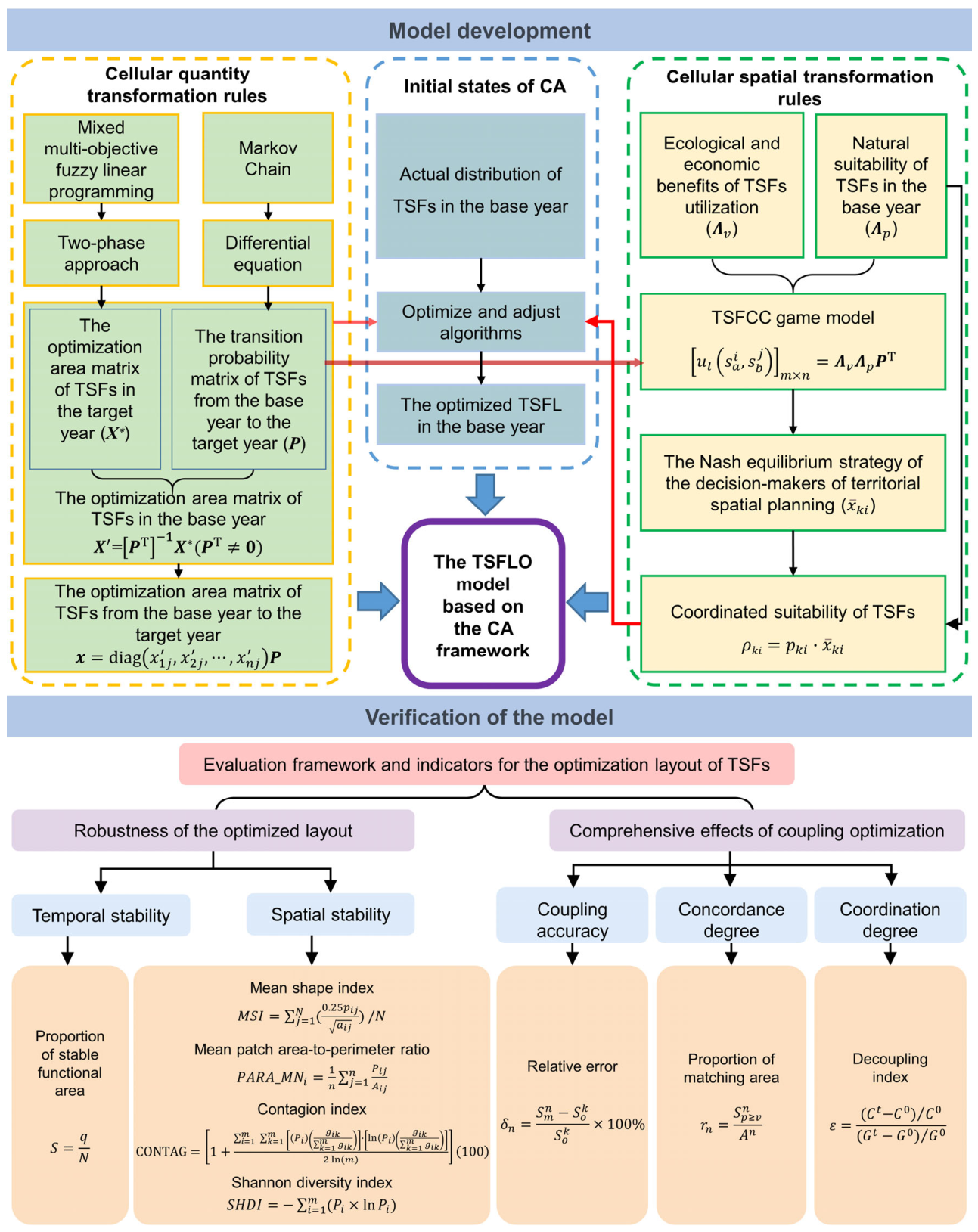
TSFLO consists of four modules (Figure 2): cellular quantity transition rules, cellular spatial transition rules, CA initial-state inversion, and result evaluation. These modules are sequentially connected through intermediate variables. The cellular quantity transition rule module takes low-carbon development and economic growth objectives, socioeconomic and resource constraints, and historical functional transition probabilities as inputs. Multi-objective fuzzy linear programming determines the optimal quantitative structure of the target year (${\mathit{X}}^{*}$), while the non-homogeneous Markov process derives the transition probability matrix ($\mathit{P}$) from the base year to the target year. Based on these results, the model inversely derives the optimal quantitative structure of the base year (${\mathit{X}}^{\prime }$) and calculates the optimal transition area matrix ($\mathit{x}$). The transition probability matrix ($\mathit{P}$) is further transferred to the cellular spatial transition rule module, ensuring that quantity optimization and spatial allocation are based on consistent functional transition information.

The cellular spatial transition rule module uses natural suitability, the low-carbon and economic benefits of functional utilization, and the transition probability matrix ($\mathit{P}$) as inputs. Based on these inputs, the game-theoretic model calculates the optimal selection probabilities of planning decision-makers for different territorial spatial functions and uses these probabilities to modify natural suitability, producing coordinated suitability (${\rho }_{ki}$). The coordinated suitability serves as both the spatial transition rule for CA simulation and the basis for determining cellular allocation priorities during the adjustment of the base-year layout. The CA initial-state inversion module receives the actual base-year layout, the optimal base-year quantitative structure (${\mathit{X}}^{\prime }$), and coordinated suitability (${\rho }_{ki}$), and outputs an optimized layout consistent with the optimal quantitative structure of the base year. This optimized layout is used as the initial CA state and, together with the optimal transition area matrix ($\mathit{x}$) and coordinated suitability (${\rho }_{ki}$), drives CA iterations to generate the optimized target-year layout.

The result evaluation module receives the optimized target-year layout, the optimal target-year quantitative structure, functional suitability, low-carbon and economic indicators, and the outputs of the PLUS model under identical parameter settings. The evaluation includes layout stability, quantitative coupling errors, suitability matching performance, and the coordination between low-carbon development and economic growth. The information linkages among modules are primarily established during model construction. Specifically, the optimal target-year quantitative structure constrains the base-year quantitative structure and CA initial state through the Markov state-transition equation, while the game-theoretic model modifies spatial transition rules through interactions between planning decision-makers and the territorial spatial function system. The result evaluation module is used for post hoc diagnosis and model comparison. The current framework does not incorporate an iterative updating mechanism in which evaluation results are automatically fed back to the preceding three modules, nor is it intended to assess the predictive accuracy of the actual spatial layouts in the target years.

Figure 2. TSFLO framework and data flows among the four modules.

Figure 2. TSFLO framework and data flows among the four modules.

3.2.1. Cellular Quantity Transformation Rules

(1) Quantitative composition optimization of TSFs in the target year

Based on fuzzy multi-objective decision-making theory, we construct a model for optimizing the quantitative composition of TSFs with the goal of coordinating low-carbon and economic growth. The model takes the economic benefits of TSF use as the benefit target, carbon emissions as the cost target, and the area of each TSF use type as the decision variable. Further, the model takes the production outputs of secondary and tertiary sectors, the urban–rural population distribution, and grain production as fuzzified constraints, and the ecological space boundary as a deterministic constraint to form a mixed multi-objective fuzzy linear programming model. With this model, we can obtain the optimal area of TSF use for coordinated low-carbon and economic growth. The model is formulated as follows:

$${\displaystyle \genfrac{}{}{0pt}{}{\begin{array}{c}\tilde{\max }\tilde{Z}=\tilde{\mathit{C}}\mathit{X}\\ \tilde{\min }\tilde{W}=\widetilde{{\mathit{C}}^{\prime }}\mathit{X}\end{array}}{s.t.\left\{\begin{array}{c}\tilde{\mathit{A}}\mathit{X}\le \tilde{\mathit{b}}\\ {\mathit{A}}^{\prime }\mathit{X}\le {\mathit{b}}^{\prime }\\ {\displaystyle {\sum }_{j=1}^n}{x}_j=S\\ \mathit{l}\le \mathit{X}\le \mathit{u}\end{array}\right.}}$$

(1)

where $\tilde{Z}$ is defined as an income-type objective function that quantifies the aggregate economic benefits derived from the utilization of TSFs; $\tilde{W}$ is defined as a cost-type objective function capturing the aggregate carbon emissions associated with TSF utilization. The vector $\tilde{\mathit{C}}=\left(\widetilde{c_1},\widetilde{c_2},\cdots ,\widetilde{c_n}\right)$ represents the value coefficients corresponding to the economic benefits per unit area of TSF utilization. The vector $\widetilde{{\mathit{C}}^{\prime }}=\left(\widetilde{c_1^{\prime }},\widetilde{c_2^{\prime }},\cdots ,\widetilde{c_n^{\prime }}\right)$ represents the value coefficients associated with carbon emissions per unit area resulting from TSF utilization; $\mathit{X}:=\left\{{\left(x_1,x_2,\cdots x_n\right)}^{\mathrm{T}}\in {\mathbb{R}}^{+n}\right\}$ represents the decision variable matrix, indicating the spatial area of different TSFs across countries; $\tilde{\mathit{A}}:=\left\{\left(\widetilde{a_{ij}}\right)\in {\mathbb{R}}^{k\times n}\right\}$ represents the technical coefficient matrix of the fuzzy constraint conditions; $\tilde{\mathit{b}}=\left\{{\left(\widetilde{b_1},\widetilde{b_2},\cdots ,\widetilde{b_k}\right)}^{\mathrm{T}}\in {\mathbb{R}}^k\right\}$ represents the resource limit matrix of the fuzzy constraint conditions; ${\mathit{A}}^{\prime }=\left\{\left(a_{ij}^{\prime }\right)\in {\mathbb{R}}^{\left(m-k\right)\times n}\right\}$ and ${\mathit{b}}^{\prime }=\left\{{\left(b_{k+1}^{\prime },b_{k+2}^{\prime },\cdots ,b_m^{\prime }\right)}^{\mathrm{T}}\in {\mathbb{R}}^{m-k}\right\}$ respectively represent the technical coefficient matrix and resource limit matrix of ecological spatial constraints; $S$ is the total area of territorial space; and $\mathit{l}:=\left\{{\left(l_1,l_2,\cdots l_n\right)}^{\mathrm{T}}\in {\mathbb{R}}^{+n}\right\}$ and $\mathit{u}:=\left\{{\left(u_1,u_2,\cdots u_n\right)}^{\mathrm{T}}\in {\mathbb{R}}^{+n}\right\}$ respectively represent the lower and upper bounds of decision variables.

The model for optimizing the quantitative composition of TSFs described in Equation (1) is a hybrid multi-objective fuzzy linear programming model with fuzzy and deterministic constraints. Therefore, we use a previously proposed hybrid multi-objective fuzzy linear programming solution [7] to convert this model into the easy-to-solve single-objective linear programming model:

$${\displaystyle \genfrac{}{}{0pt}{}{\max \overline{\phi }=\frac{1}{2}\left({\phi }_z+{\phi }_w\right)}{\begin{array}{cc}s.t.& \left\{\begin{array}{l}\rho \le {\phi }_z\le {\mu }_{\tilde{Z}}\left({\tilde{Z}}_{\alpha }^R\right)\\ \rho \le {\phi }_w\le {\mu }_{\tilde{W}}\left({\tilde{W}}_{\alpha }^L\right)\\ {\tilde{\mathit{A}}}_{\alpha }^L\mathit{X}\le {\tilde{\mathit{b}}}_{\alpha }^R\\ \mathit{X}\in {\mathit{X}}_{\alpha }\\ {\phi }_z,{\phi }_w\in \left[\mathrm{0,1}\right]\end{array}\right.\end{array}}}$$

(2)

where $\overline{\phi }$ is the objective function, representing the arithmetic mean operator; ${\phi }_z$ and ${\phi }_w$ represent the fuzzy satisfaction of cost-related and benefit-related objectives, respectively; $\tilde{Z}$ represents the fuzzy desires corresponding to the income-type objectives; $\tilde{W}$ represents the fuzzy desires corresponding to the cost-type objectives; $\alpha \in \left[\mathrm{0,1}\right]$ represents the possibility of the fuzzy parameter in the solution; ${\tilde{Z}}_{\alpha }^R$ and ${\tilde{W}}_{\alpha }^L$ respectively represent the right and left boundaries of the benefit-type objective ${\tilde{Z}}_{\alpha }$ and the cost-type objective ${\tilde{W}}_{\alpha }$ under the $\alpha$ cut-off condition; ${\mu }_{\tilde{Z}}\left({\tilde{Z}}_{\alpha }^R\right)$ and ${\mu }_{\tilde{W}}\left({\tilde{W}}_{\alpha }^L\right)$ represent the membership functions corresponding to the fuzzy desires $\tilde{Z}$ and $\tilde{W}$, respectively; ${\tilde{\mathit{b}}}_{\alpha }^R$ and ${\tilde{\mathit{A}}}_{\alpha }^L$ respectively represent the right and left boundaries of the fuzzy resource constraints and technical coefficients under the α cut-off condition; $\mathit{X}\in {\mathit{X}}_{\alpha }$ represents the deterministic constraints of the optimization model for the quantitative composition of TSFs; and $\rho$ represents the satisfaction of decision makers under the dual constraints of fuzzy objectives and fuzzy parameters. According to the Bellman–Zaden principle [48], $\rho =\mathrm{m}\mathrm{i}\mathrm{n}\left\{\alpha ,\phi \right\}$. Ideally, ${{\rho =\phi }^{*}=\alpha }^{*}$, where the optimal level ${\alpha }^{*}$ and the overall satisfaction value ${\phi }^{*}$ can be obtained by solving the following linear programming model:

$${\displaystyle \genfrac{}{}{0pt}{}{\mathrm{m}\mathrm{a}\mathrm{x}\phi }{\begin{array}{cc}s.t.& \left\{\begin{array}{l}\phi \le {\mu }_{\tilde{Z}}\left({\tilde{Z}}_{\alpha }^R\right)\\ \phi \le {\mu }_{\tilde{W}}\left({\tilde{W}}_{\alpha }^L\right)\\ {\tilde{\mathit{A}}}_{\alpha }^L\mathit{X}\le {\tilde{\mathit{b}}}_{\alpha }^R\\ \mathit{X}\in {\mathit{X}}_{\alpha }\\ 0\le \phi \le 1\end{array}\right.\end{array}}}$$

(3)

The $\alpha$ level is an endogenous solution variable in the two-stage fuzzy decision-making process rather than a predefined external parameter. In the first stage, the maximum objective satisfaction degree $\phi \left(\alpha \right)$ corresponding to different $\alpha$-cut levels is solved within the range of $\alpha \in \left[\mathrm{0,1}\right]$, and the Bellman–Zadeh principle is applied to calculate $\rho \left(\alpha \right)=\mathrm{m}\mathrm{i}\mathrm{n}\left\{\alpha ,\phi \left(\alpha \right)\right\}$. The $\alpha$ value that maximizes $\rho \left(\alpha \right)$ is identified as the optimal possibility level ${\alpha }^{*}$, and the corresponding maximum overall satisfaction degree is denoted as ${\rho }^{*}$. At the ideal equilibrium point, ${\alpha }^{*}=\phi \left({\alpha }^{*}\right)={\rho }^{*}$. In the second stage, $\alpha$ and $\rho$ are fixed, with $\rho$ serving as the common lower bound for the satisfaction degrees of the benefit objective ${\phi }_z$ and the cost objective ${\phi }_w$. The fully compensatory arithmetic mean satisfaction degree $\overline{\phi }=\left({\phi }_z+{\phi }_w\right)/2$ is then maximized to obtain the non-dominated quantitative structure $\mathit{X}$ adopted in the subsequent analysis of this study from the acceptable solution set identified in the first stage [7,29,48]. Therefore, the final quantitative structure is not selected from several artificially specified $\alpha$ scenarios; instead, $\alpha$ and $\mathit{X}$ are jointly determined by the two-stage algorithm.

(2) Probability matrix for the transfer of TSFs from the baseline year to the target year

Using the Markov chain approach, we calculate the TSF transition probability matrix ${\left(p_{ij}\right)}_{n\times n}\left(i,j=\mathrm{1,2},\cdots ,n\right)$ for any given time period in the past ($t$). Assuming that the transition probability $p_{ij}$ is a function $p_{ij}\left(t\right)$ that continuously changes over time t, and likewise that the rate of change $r$ per unit time is a function $r_{ij}\left(t\right)$ that changes over time, a differential equation can be obtained that describes the law of transition probability variation and its definite solution conditions:

$$\begin{array}{c}{\displaystyle \frac{d{p}_{ij}}{dt}}=r_{ij}\left(t\right)p_{ij}\\ {\left.p_{ij}\right|}_{t=0}={\left(p_{ij}\right)}_0,{\left.r_{ij}\right|}_{t=0}={\left(r_{ij}\right)}_0\end{array}$$

(4)

Solving the definite solution problem (Equation (4)), we can obtain

$$p_{ij}\left(t\right)=B{e}^{\int r_{ij}\left(t\right)dt}$$

(5)

where $B$ is an undetermined constant, and the initial value is ${\left(p_{ij}\right)}_0.$ This study does not assume that the functional transition probabilities from 2010 to 2020 remain constant. Instead, the transition probabilities for consecutive years are calculated separately, and $p_{ij}$ is expressed as a function of time $t$. Therefore, different time periods use different transition probability matrices, and Equations (6) and (7) further normalize and accumulate the matrices for each period.

Using Equation (5), we calculate the probability of TSF transitions from the baseline year to the target year in different time periods, denoted as $p_{ij}^{t^{\prime }}\left(t^{\prime }=t+1,t+1,\cdots ,T-1\right)$. Based on this, we calculate the probability matrix $\overline{{\mathit{P}}^{t^{\prime }}}$ of TSF transitions from the baseline year to the target year in different time periods:

$$\overline{{\mathit{P}}^{t^{\prime }}}=\mathrm{d}\mathrm{i}\mathrm{a}\mathrm{g}\left(1/{\mathsf{\Sigma }}_j{p}_{1j}^{t^{\prime }},1/{\mathsf{\Sigma }}_j{p}_{2j}^{t^{\prime }},\cdots ,1/{\mathsf{\Sigma }}_j{p}_{nj}^{t^{\prime }}\right){\mathit{P}}^{t^{\prime }}$$

(6)

where ${\mathsf{\Sigma }}_j{p}_{nj}^{t^{\prime }}$ represents the total probability of an $n$-class TSF transfer for the $t^{\prime }$-th time period, and ${\mathit{P}}^{t^{\prime }}={\left(p_{ij}^{t^{\prime }}\right)}_{n\times n}$ represents the probability matrix of TSF transfers during the $t^{\prime }$ period.

Finally, we calculate and determine the TSF probability matrix $\mathit{P}$ from the baseline year to the target year:

$$\mathit{P}={\mathsf{\Pi }}_{t^{\prime }}\overline{{\mathit{P}}^{t^{\prime }}}$$

(7)

Equations (4)–(7) are used to derive the cumulative transition probability matrix ($\mathit{P}$) from the base year to the target year. Equations (4) and (5) fit the temporal evolution of transition pathways among different territorial spatial functions based on historical transition probabilities. Equation (6) normalizes the transition probability matrices for different periods, and Equation (7) multiplies the probability matrices across consecutive periods to obtain the cumulative transition probability matrix between the base year and the target year. The resulting matrix $\mathit{P}$ is subsequently used to inversely derive the optimal quantitative structure of the base year and serves as an input for constructing the game payoff matrix.

(3) Calculation of the optimal transfer area matrix of TSFs from the baseline year to the target year

Assuming that the optimization area matrix of TSFs for the baseline year and the target year are ${\mathit{X}}^{\prime }={\left(x_{ij}^{\prime }\right)}_{n\times 1}$ and ${\mathit{X}}^{\mathrm{*}}={\left(x_{ij}^{\mathrm{*}}\right)}_{n\times 1}$, respectively, the optimization area matrix of TSFs from the baseline year to the target year is $\mathit{x}={\left(x_{ij}\right)}_{n\times n}$:

$$\mathit{x}=\mathrm{d}\mathrm{i}\mathrm{a}\mathrm{g}\left(x_{1j}^{\prime },x_{2j}^{\prime },\cdots ,x_{nj}^{\prime }\right)\mathit{P}$$

(8)

where $x_{1j}^{\prime },x_{2j}^{\prime },\cdots ,x_{nj}^{\prime }$ represent the elements of the matrix ${\mathit{X}}^{\prime }$ of the optimization area matrix of TSFs in the baseline year, derived as follows:

$${\mathit{X}}^{\prime }={\left[{\mathit{P}}^{\mathrm{T}}\right]}^{-1}{\mathit{X}}^{\mathrm{*}}\left({\mathit{P}}^{\mathrm{T}}\ne 0\right)$$

(9)

Equations (8) and (9) transform the target-year quantity optimization results into the quantity transition rules required by the CA model. Equation (9) inversely derives the optimal quantitative structure of the base year (${\mathit{X}}^{\prime }$) based on the optimal quantitative structure of the target year (${\mathit{X}}^{\mathrm{*}}$) and the cumulative transition probability matrix ($\mathit{P}$). Equation (8) further calculates the optimal transition area matrix ($\mathit{x}$) from the base year to the target year. The derived ${\mathit{X}}^{\prime }$ constrains the reconstruction of the CA initial state, whereas $\mathit{x}$ determines the number of cells that need to be transferred among different territorial spatial functions during CA iterations.

3.2.2. Cellular Spatial Transformation Rules

Assume that territorial spatial functional conflict coordination (TSFCC) is a spatial intervention implemented by humans (territorial spatial planner) on natural systems (i.e., TSFs) for the purpose of maintaining the harmonized development of humans and nature. It abstracts conflict coordination as a zero-sum game played by a territorial spatial planner and the system of TSFs, and establishes a TSFCC game model. The zero-sum assumption is introduced to describe the competitive relationship among dominant function choices within the same spatial unit, rather than to imply that the overall interests of human development and ecological conservation are necessarily opposed. In this game, the TSF system is a mathematical representation of natural suitability, functional transition dynamics, and eco-economic feedback rather than an intentional decision-making actor in the real world. Since each spatial unit can be assigned only one dominant function, increasing the selection probability of one function inevitably reduces the available selection space for other functions. Under practical conditions, pure-strategy Nash equilibria are often difficult to obtain. Therefore, this study uses a mixed-strategy Nash equilibrium. The selection probabilities of the different functions represent the optimal mixed strategies of the territorial spatial planner and the TSF system [49]. For a given spatial unit, the equilibrium probabilities characterize the likelihood that each territorial function is selected as the dominant TSF under the expected payoffs. Within the specified payoff matrix and strategy spaces, these probabilities form an equilibrium strategy profile in which neither player can increase its expected payoff by changing its strategy unilaterally. From the perspective of game theory, the Nash equilibrium includes the strategy (${\overline{X}}_k$) of the territorial spatial planner and strategy (${\overline{Y}}_k$) of the system of TSFs. The former, ${\overline{X}}_k$, denotes the optimal strategy selected by humans to resolve TSFCs—that is, the corresponding set of choice probabilities that maximize the expected outcome for each TSF. The latter, ${\overline{Y}}_k$, represents the modeled response of the TSF system to the optimal strategy of the territorial spatial planner. It captures the feedback of natural suitability, functional transitions, and eco-economic conditions on the planning decision. The Nash equilibrium therefore describes the equilibrium of the specified game and does not demonstrate that the resulting spatial layout is robust to parameter changes or external disturbances. Therefore, ${\overline{X}}_k$, which represents the planner’s optimal strategy, is used to modify the natural suitability of the TSFs. The resulting coordinated suitability accounts for functional conflicts and is used to construct the cellular spatial transition rule. This rule reduces the influence of functional conflicts on spatial allocation. The evaluation model is formulated as follows:

$${\rho }_{ki}=p_{ki}·{\overline{x}}_{ki}$$

(10)

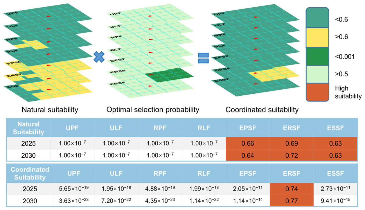
where ${\rho }_{ki}$ and $p_{ki}$ represent the coordinated suitability of TSFs and the natural suitability of TSFs of the $i$-th category of TSF belonging to the $k$-th spatial unit. Here, $p_{ki}$ is determined using the double evaluation method described in Section 3.1 with the spatial unit as the evaluation unit [50,51]; ${\overline{x}}_{ki}$ represents the optimal selection probability of the $i$-th type of TSF for the $k$-th spatial unit by the territorial spatial planner (${\overline{x}}_{ki}\in {\overline{X}}_k$). The optimal selection probabilities are determined through the TSFCC game model. Equation (10) adopts a multiplicative adjustment rather than a weighted summation; therefore, no additional weights need to be manually assigned between natural suitability and the optimal selection probabilities. Natural suitability provides the basis for spatial allocation, while the selection probabilities derived from the mixed-strategy Nash equilibrium modify this suitability according to the functional conflict coordination results. The strategy formulation of the TSFCC game model is as follows:

$$G=\left\{S_l;u_l\left(s_l^k\right)\right\}$$

(11)

where $G$ represents the TSFCC game model; $l$ represents the participants in the game model, such that $l\in \left\{a,b\right\}$, with $a$ representing the territorial spatial planner; $b$ represents the TSF system; and $S_l$ represents the strategy set of participant $l$, defined as $S_l=\left\{{s_l^1,s_l^2,\cdots ,s_l^k,\cdots ,s}_l^n\right\}$, where $s_l^k$ denotes the $k$-th specific strategy of participant $l$ (i.e., a TSF type). The set $\left\{{s_l^1,s_l^2,\cdots ,s_l^k,\cdots ,s}_l^n\right\}$ represents the strategy set of participant $l$. If each participant chooses one specific strategy, then the vector $\mathit{s}=\left(s_a^i,s_b^j\right)$ represents a strategy combination. Finally, $u_l\left(s_l^k\right)$ represents the utility function of the participant, which indicates a certain level of utility obtained by the participant under a specific strategy combination, where $k$ represents the strategy that the participant can choose.

According to game theory, the payoff of the territorial spatial planner depends both on their individual strategies regarding the different TSFs and on the responses of the TSF system to the strategies selected by the territorial spatial planner. Thus, the utility function for the game participants can be defined as $u_l\left(s_l^k\right)=u_l\left(s_a^i,s_b^j\right)$. Due to the complexity of the system of TSFs, it is difficult for model $G$ to achieve a pure-strategy Nash equilibrium under practical conditions. Instead, what is commonly observed is a mixed-strategy Nash equilibrium. The linear programming method is an effective method for solving the mixed-strategy Nash equilibrium of zero-sum games [49]. We assume that $\mathit{A}={\left[u_a\left(s_a^i,s_b^j\right)\right]}_{m\times n}$ and $E_a\left(\mathit{X},\mathit{Y}\right)={\mathit{X}}^{\mathrm{T}}\mathit{A}\mathit{Y}$ respectively represent the payoff matrix and expected payoff of the territorial spatial planner. Here, $\mathit{X}={\left(x_1,x_2,\cdots ,x_i,\cdots ,x_m\right)}^{\mathrm{T}}\left(i=\mathrm{1,2},\cdots ,m;x_i\ge 0;{\sum }_{i=1}^m{x}_i=1\right)$ and $\mathit{Y}={\left(y_1,y_2,\cdots ,y_j,\cdots ,y_n\right)}^{\mathrm{T}}\left(j=\mathrm{1,2},\cdots ,n;y_j\ge 0;{\sum }_{i=1}^n{y}_i=1\right)$ represent the respective choices of participants $a$ and $b$ for $s_a^i$ and $s_b^j$—that is, the mixed strategies. In a mixed strategy of zero-sum games, the aim of the territorial spatial planner is to determine a mixed strategy $\overline{\mathit{X}}={\left({\overline{x}}_1,{\overline{x}}_2,\cdots ,{\overline{x}}_i,\cdots ,{\overline{x}}_m\right)}^{\mathrm{T}}\left({\overline{x}}_i\ge 0;i=\mathrm{1,2},\cdots ,m;{\sum }_{i=1}^m{\overline{x}}_i=1\right)$, such that without regard to the strategy $\mathit{Y}$ adopted by the TSFs, these decision-makers can ensure maximum returns given that the opponent plays their minimum payoff strategy, that is: $\underset{{\overline{x}}_i\in \overline{\mathit{X}}}{\max }\underset{y_j\in \mathit{Y}}{\min }{\overline{\mathit{X}}}^{\mathrm{T}}\mathit{A}\mathit{Y}$. Let ${\mathit{e}}_j$ be the unit row vector that has only the $j$-th component equal to 1, while all other components are 0. Let ${\mathit{E}}_j={\mathit{X}}^{\mathrm{T}}\mathit{A}{\mathit{e}}_j^{\mathrm{T}}$, and then $\underset{x_i\in \mathit{X}}{\max }\underset{y_j\in \mathit{Y}}{\min }{\mathit{X}}^{\mathrm{T}}\mathit{A}\mathit{Y}=\underset{x_i\in \mathit{X}}{\max }\underset{y_j\in \mathit{Y}}{\min }{\displaystyle {\sum }_{j=1}^n}{\mathit{E}}_j{y}_j$. Let $u\equiv {\mathit{E}}_k=\underset{j}{\min }{\mathit{E}}_j$. Since ${\sum }_{j=1}^n{y}_j=1$, the expression $\underset{y_j\in \mathit{Y}}{\min }{\displaystyle {\sum }_{j=1}^n}{\mathit{E}}_j{y}_j$ attains its minimum value $u$ when $y_k=1$ and $y_j=0$ for $j\ne k$. Therefore, $\underset{x_i\in \mathit{X}}{\max }\underset{y_j\in \mathit{Y}}{\min }{\sum }_{j=1}^n{\mathit{E}}_j{y}_j\equiv \underset{x_i\in \mathit{X}}{\max }u$. Hence, $\overline{\mathit{X}}$ is obtained as the solution to the following linear programming problem:

$$\begin{array}{c}\max u\\ s.t.\left\{\begin{array}{l}\begin{array}{l}{\mathit{E}}_j\ge u\\ {\displaystyle \sum _{i=1}^m}{x}_i=1\end{array}\\ \begin{array}{l}{x}_i\ge 0\\ i=\mathrm{1,2},\cdots ,m; j=\mathrm{1,2},\cdots ,n\end{array}\end{array}\right.\end{array}$$

(12)

Since ${\mathit{E}}_j={\mathit{X}}^{\mathrm{T}}\mathit{A}{\mathit{e}}_j^{\mathrm{T}}={\sum }_{i=1}^m{u}_a\left(s_a^i,s_b^j\right)x_i\left(j=\mathrm{1,2},\cdots ,n\right)$, the above linear programming problem (Equation (12)) can be expressed as

$$\begin{array}{c}\max u\\ s.t.\left\{\begin{array}{c}{\sum }_{i=1}^m{u}_a\left(s_a^i,s_b^j\right)x_i\ge u\hfill \\ {\sum }_{i=1}^m{x}_i=1\hfill \\ x_i\ge 0\hfill \\ i=\mathrm{1,2},\cdots ,m;j=\mathrm{1,2},\cdots ,n\hfill \end{array}\right.\end{array}$$

(13)

Equations (10)–(13) describe how the results of functional conflict coordination are transformed into spatial transition rules. Equation (10) integrates the natural suitability ($p_{ki}$) with the optimal selection probability (${\overline{x}}_{ki}$) of planning decision-makers to derive the coordinated suitability (${\rho }_{ki}$). Equations (11)–(13) formulate a zero-sum game between planning decision-makers and the territorial spatial function system and solve the mixed strategies of planning decision-makers under different responses of the functional system. The resulting optimal strategy (${\overline{X}}_k$) provides ${\overline{x}}_{ki}$, allowing both planning decisions and responses from the natural system to be incorporated into the calculation of coordinated suitability.

Let $\overline{\mathit{X}}$ denote the optimal choice probability vector of TSFs for the $k$-th spatial unit by the territorial spatial planner. Then, the Nash equilibrium of these decision-makers can be expressed as ${\overline{X}}_k=\left\{{\overline{x}}_1,{\overline{x}}_2,\cdots ,{\overline{x}}_m\right\}$. Similarly, a linear programming model can be established to solve the mixed strategy $\overline{\mathit{Y}}={\left({\overline{y}}_1,{\overline{y}}_2,\cdots ,{\overline{y}}_j,\cdots ,{\overline{y}}_n\right)}^{\mathrm{T}}\left({\overline{y}}_j\ge 0;j=\mathrm{1,2},\cdots ,n;{\sum }_{i=1}^n{\overline{y}}_i=1\right)$, in order to obtain the Nash equilibrium strategy ${\overline{Y}}_k=\left\{{\overline{y}}_1,{\overline{y}}_2,\cdots ,{\overline{y}}_n\right\}$ for the TSF system. Thus, the mixed-strategy Nash equilibrium solution of model $G$ can be obtained and is denoted as $\left(\overline{\mathit{X}},\overline{\mathit{Y}}\right)$, with the payoff (utility) given by ${\overline{\mathit{X}}}^{\mathrm{T}}\mathit{A}\overline{\mathit{Y}}$.

3.2.3. Initial States of CA

According to the law of TSF transfers (Equation (8)), there must be an optimal base-year TSF area corresponding to the target year’s optimal scale of TSFs. However, this area usually differs from the actual area in the baseline year. To address this issue, we generate a functional layout consistent with the optimal quantitative composition of the baseline year (i.e., the optimized layout of TSFs in the baseline year) as the initial state of the cell based on coordination and suitability. We generate this layout by adjusting the actual distribution of functions in the baseline year. The specific steps are as follows:

Step 1: Apply the principle of permutation and combination to generate all possible combinations of TSF adjustment sequences.

Step 2: Select any adjustment sequence combination, sort the functional types to be adjusted in descending order according to their coordination suitability, and prioritize the allocation of spatial units with the current status of that function to the target type. If the allocated area reaches the optimal area for that function in the baseline year, then proceed to the next functional distribution adjustment; if not, proceed to Step 3.

Step 3: For functional types that do not meet the standards, allocate space from other functional types in order of coordination suitability until the optimal area is reached. Then, proceed to adjust the next functional type.

Step 4: Repeat steps 2 and 3 to process all combinations with adjusted sequences in order, generating the base-year functional distribution adjustment results for each combination.

Step 5: Convert the candidate layouts generated from all functional adjustment sequences into raster maps. Steps 2 through 4 ensure that every candidate layout contains the optimal baseline-year number of cells for all seven functions, as determined by Equation (9). This step therefore screens only the spatial distribution and does not reassess the quantitative composition. Compare each candidate with the actual 2020 TSF distribution shown in Figure S4 of Supplementary Information S7. The comparison considers the principal concentration areas of each function, the overall direction of its spatial distribution, and whether its basic spatial organization is clustered or dispersed. Any candidate consistent with the actual baseline layout may be used as the CA initial state. A candidate is discarded if the principal distribution of any function shifts to an area that is clearly inconsistent with the actual 2020 pattern.

3.3. Comparative Evaluation of the TSFLO and PLUS Optimization Results

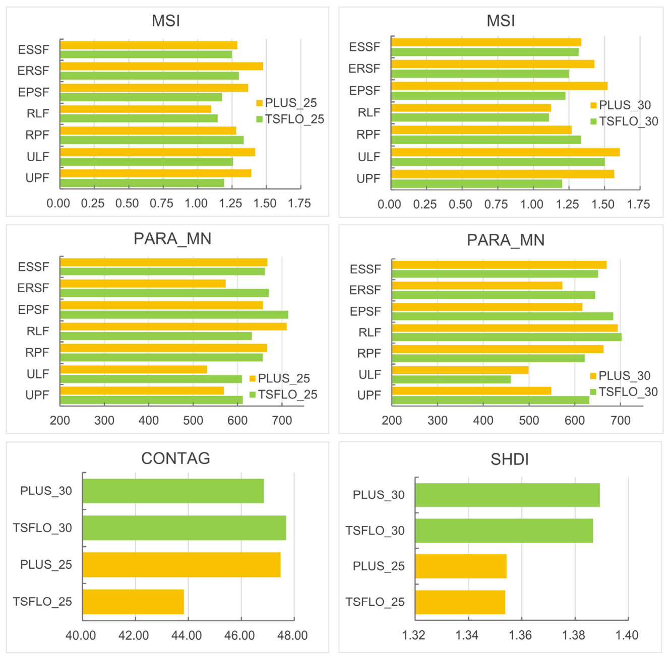
The PLUS model integrates the Land Expansion Analysis Strategy (LEAS) with the Multi-type Random Patch Seed Cellular Automata (CARS) and has been widely used for land-use change simulation [9]. To compare the stability characteristics and coupled optimization performance of the layouts generated by the two models, this study establishes an evaluation framework from two perspectives: layout stability and overall coupled optimization performance. The specific indicators are provided in Table S1 of Supplementary Information S1. In this study, layout stability refers to the extent to which an optimized scenario, under the same target year and identical evaluation conditions, responds to the target quantitative structure and spatial suitability requirements while maintaining continuity with the baseline functional layout and producing a relatively regular, connected, and not excessively fragmented spatial pattern. Layout stability includes temporal stability and spatial stability. Temporal stability is evaluated using the Stable Functional Area Ratio (SFAR), which measures the extent to which functional types are retained in the optimized layout relative to the 2020 baseline layout. Spatial stability is evaluated using the Mean Shape Index (MSI), Mean Perimeter–Area Ratio (PARA_MN), Contagion Index (CONTAG), and Shannon Diversity Index (SHDI), which characterize patch shape, fragmentation, aggregation and connectivity characteristics, and landscape composition, respectively. Overall coupled optimization performance is evaluated using the relative error of the quantitative structure, the proportion of areas matching high-coordinated-suitability areas, and the decoupling index. TSFLO and PLUS use the same baseline data, spatial resolution, target years, and basic CA parameters, and are compared separately for 2025 and 2030 at the same target year. Both optimization scenarios use 2020 as the common baseline year but separately use the target-year-specific quantitative structure, Markov transition matrix, CA initial state, and number of iterations; therefore, they constitute independent optimization scenarios under different planning horizons. The difference in SFAR between the two target years is not used to judge the relative performance of the models. No single stability metric is used to determine the overall conclusion; instead, each metric is interpreted together with quantitative coupling accuracy and spatial suitability matching results. This comparison is intended to evaluate the relative stability characteristics and coupled performance of the two optimization scenarios under the specified benchmark settings, rather than to assess predictive validity or whether model outputs remain invariant under changes in parameters. This study did not conduct historical hindcasting against independently observed functional layouts for a historical target year. Nor did it conduct systematic sensitivity or perturbation analyses by varying the fuzzy parameter ranges, Markov transition scenarios, spatial resolution, or CA settings. The comparison therefore characterizes the relative layout stability and coupled performance of the two models only under the data, evolutionary scenarios, and model settings used in this study.

4. Empirical Application to the Study Area

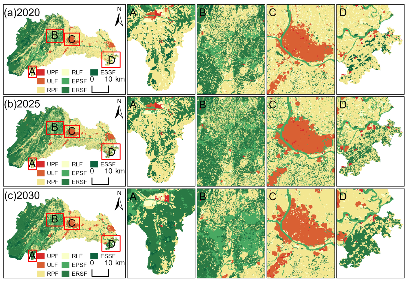
To demonstrate the application of TSFLO to territorial spatial function layout optimization under the coordinated objectives of low-carbon development and economic growth, Qionglai City, China, was selected as the case study area. Based on the existing territorial spatial function classification results, 2020 was used as the baseline year, and TSFLO was applied to generate optimized territorial spatial function layouts for 2025 and 2030 [52]. These two layouts represent forward-looking planning scenarios under the specified optimization objectives, constraints, and functional evolution scenarios, rather than predictions of the actual layouts in the target years. The optimization performance was evaluated using the indicators established in Section 3.3, and the results were compared with those generated by PLUS under identical parameter settings.

4.1. Study Area and Data Sources

4.1.1. Description of the Study Area

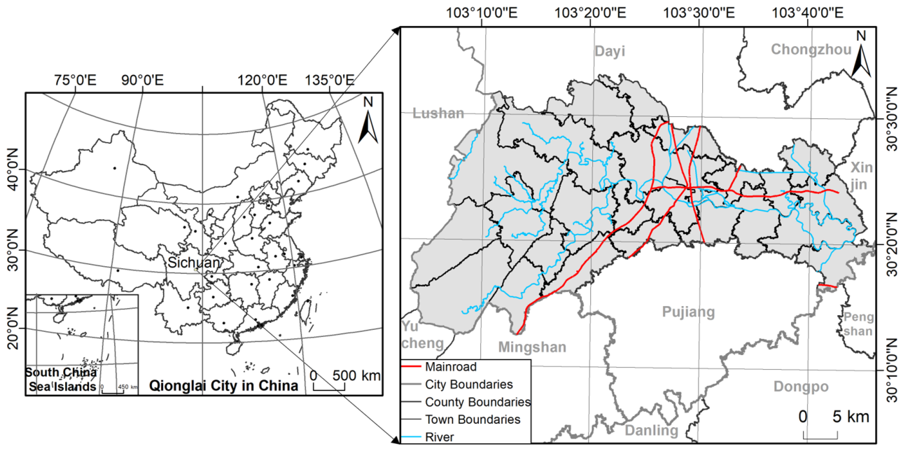
Qionglai City (30°12′ N–30°33′ N, 103°04′ E–103°45′ E) is located in China in the transition zone between the Chengdu Plain and the Longmen Mountains, with a total area of 1377 km² (Figure 3). The terrain is higher in the northwest and lower in the southeast, with elevations ranging from 451 to 1991 m above sea level. The main landforms are plains (311.36 km²), mountains (817.79 km²) and hills (245.98 km²). Plain areas are distributed in the eastern and northeastern parts of the city. Mountainous areas are primarily found in the Wumian Mountain and Changqiu Mountain regions in the south, as well as in the southern extension of the Longmen Mountain range in the west. Hilly areas are scattered along the north-western edge of the central part of the study area. The city possesses relatively abundant water resources, with transit rivers stretching 271.25 km in total length. Qionglai experiences a subtropical humid monsoon climate, with an average annual temperature of 16.3 °C and an average annual precipitation of 1117.3 mm. The predominant soil types are alluvial soil and purple soil. The forest vegetation belongs to the subtropical evergreen broad-leaved forest type and is mainly distributed in the mid-low mountain areas of the northwest and the central hilly areas. This complex combination of terrain and landform characteristics, together with pronounced spatial heterogeneity, provides an ideal empirical space for adjusting the territorial spatial functional layout to mitigate the contradiction between carbon emission reduction and economic growth.

Qionglai City encompasses major territorial spatial function types, including the urban production function (UPF), urban living function (ULF), rural production function (RPF), rural living function (RLF), ecological supply services function (EPSF), ecological regulation services function (ERSF), and ecological support services function (ESSF) [52]. The city has simultaneously experienced urbanization, industrial growth, demographic changes, and carbon emission pressures, while facing notable demands for ecological space conservation. These characteristics make Qionglai suitable as a methodological application case for territorial spatial function layout optimization under the joint constraints of low-carbon development and economic growth. This study does not regard Qionglai as an empirical representative of all developing countries, nor does it use this case to demonstrate the predictive validity of the model in other regions. Before applying the model to other regions, it needs to be recalibrated according to local functional classifications, data conditions, parameter ranges, and policy constraints.

Figure 3. Geographical location, administrative divisions, and major roads of the study area.

Figure 3. Geographical location, administrative divisions, and major roads of the study area.

4.1.2. Data Acquisition and Data Processing

This study compiled the multisource spatial data required for territorial spatial function layout optimization and for comparing the scenarios generated by TSFLO and PLUS. The specific data sources are listed in

Table 1. Data types and sources.

Data Type	Data Name	Time Section (Year)	Spatial Resolution	Data Source
Raster data	Digital Elevation Model (DEM)	2020	12.5 m	91 satellite map assistant (https://www.91weitu.com/, accessed before 27 July 2026)
	Net primary productivity of vegetation, water conservation, evapotranspiration, environmental self-purification capacity, soil conservation, habitat quality	2020	50 m	Data from Ou et al. [52]
	TSF distribution map	2009–2020	50 m	Data from Ou et al. [52]
Vector data	Administrative boundary	2020	1:5000	Land survey results (Key laboratory of investigation, monitoring, protection and utilization of cropland resources, MNR, PRC)
	Land-use data	2010–2020	1:5000	Chengdu Land Survey Results Database, including the results of the Second and Third National Land Surveys and the annual territorial land-change survey results (Key Laboratory of Cultivated Land Resources Survey, Monitoring, Protection and Utilization, Ministry of Natural Resources)
	Electronic maps, including data on healthcare, education, and business services	2010–2020	1:10,000	Geographical information Monitoring Cloud Platform (http://www.dsac.cn/, accessed before 27 July 2026), Satellite mapping assistance software (91 Weitu Assistant, version 2016) (https://www.91weitu.com/, accessed before 27 July 2026)
Monitoring data	Soil organic matter content, organic phosphorus content, available potassium content, alkaline hydrolysis nitrogen content	2020	921 sample points	The project on the monitoring and evaluation of soil quality in areas under crop rotation and fallow (Sichuan Provincial Department of Agriculture and Rural Affairs)
	Soil particle composition	2020	1000 m	Geographical information monitoring cloud platform (http://www.dsac.cn/, accessed before 27 July 2026)
	Temperature, precipitation	2010–2020	County level (62 stations)	Resource and environmental science data platform (https://www.resdc.cn/, accessed before 27 July 2026)
	Radiation dose	2010–2020	County level	Meteorological science knowledge service system (https://k.data.cma.cn/, accessed before 27 July 2026)
Panel data	Number of pigs, cows, and sheep, agricultural management data	2010–2020	County level	Qionglai Statistical Yearbook
	Urban–rural populations, Gross Domestic Product (GDP)		Township level
	Comprehensive energy consumption of industrial enterprises above designated size in terms of GDP per 10,000 yuan of total industrial output value, per capita consumption of electricity, natural and liquefied gas	2010–2020	City level	Chengdu Statistical Yearbook
	Chemical oxygen demand in wastewater	2010–2020	Provincial level	China Energy Statistical Yearbook
	Cultivated land retention, ecological conservation area	2020	County level	Land use master plan of Qionglai city (2006–2020), Master plan of territorial space for Qionglai City (2021–2035)

. The land-use data directly used in this study were obtained from the Chengdu Land Survey Results Database, including the results of the Second and Third National Land Surveys and the annual territorial land-change survey results produced on the basis of these two national surveys. Remote sensing imagery was used only to prepare the survey base maps for the aforementioned land surveys and was not directly used as an independent data input to the model in this study. Grid and vector data were standardized to the WGS 1984 geographic coordinate system and the UTM projected coordinate system. The raster resolution was set to 50 m. The territorial spatial function distributions and the major gridded datasets used in this study were based on a 50 m spatial unit; therefore, a uniform spatial resolution of 50 m was adopted to maintain consistency in multisource data processing, CA decision units, and the calculation of evaluation indicators. The results were not tested for invariance across alternative spatial resolutions, and the resulting spatial layouts and model comparison conclusions were therefore specific to the 50 m analytical scale. Sample point monitoring data, including soil organic matter content, soil nutrient content and climatic factors, were converted into gridded data using Kriging interpolation. Socioeconomic data at the city and town scales were spatially processed on 50 m × 50 m vector grids following the method proposed by Ou et al. [52]. Energy consumption for urban and rural production and living, as well as the chemical oxygen demand of industrial wastewater, were calculated using parameters provided in the IPCC guidelines [53,54] and the China Energy Statistical Yearbook, following the methods described in Qin et al. [7] and Wang et al. [55].

4.2. Case Study Modeling Process

4.2.1. Construction of Cell Quantity Transformation Rules

The main steps in integrating MFLP, the Markov chain, and the differential equations to construct the cell quantity transformation rules (i.e., the transfer matrix of TSFs for 2020–2025 and 2020–2030) were as follows:

First, we used triangular fuzzy numbers (for a given membership degree $\alpha$, the $\alpha$-cut of the fuzzy number $\tilde{P}$ is represented as ${\tilde{P}}_{\alpha }=\left[{\tilde{P}}_{\alpha }^L,{\tilde{P}}_{\alpha }^R\right]=\left[P^L+\left(P^M-P^L\right)\alpha ,P^R-\left(P^R-P^M\right)\alpha \right],\alpha \in \left[\mathrm{0,1}\right]$) and linear functions [7] to determine the specific form of the fuzzy parameters and membership function for the optimized model for the quantitative composition of TSFs (Equation (1)) (the specific forms of the fuzzy objective function and constraints, as well as the calculation methods and results for fuzzy parameters and deterministic parameters in the 2025 and 2030 models, can be found in Tables S2 and S3 in the Supplementary Information, Section S2). The triangular fuzzy parameters reported in Tables S2 and S3 were not manually adjusted to obtain specific spatial outcomes. Each parameter was determined according to the data sources and calculation methods listed in Table S2. The minimum possible value ($L$), most likely value ($M$), and maximum possible value ($R$) jointly defined the uncertainty ranges considered in the quantitative optimization for 2025 and 2030. Changing $L$, $M$, and $R$ would amount to redefining the parameter uncertainty scenarios. Therefore, the quantitative optimization results in this study were conditional on the parameter ranges constructed in Tables S2 and S3. Then, the model (Equation (2)) was transformed into a solvable ordinary single-objective linear programming model (Equation (14)). Utilizing a two-stage MATLAB (R2010b, R2023b) algorithm [7] designed for this study, we next solved for the area of optimized TSFs ${\mathit{X}}^{\mathit{*}}$ for the years 2025 and 2030:

$${\displaystyle \genfrac{}{}{0pt}{}{\max \overline{\phi }=\frac{1}{2}\left({\phi }_z+{\phi }_w\right)}{\begin{array}{cc}s.t.& \left\{\begin{array}{l}\rho \le {\phi }_z\le \frac{{\displaystyle {\sum }_{j=1}^n}\left[c_j^R-\left(c_j^R-c_j^M\right)\alpha \right]x_j-{\tilde{Z}}_{\alpha }^{-}}{{\tilde{Z}}_{\alpha }^{+}-{\tilde{Z}}_{\alpha }^{-}}\\ \rho \le {\phi }_w\le \frac{{\tilde{W}}_{\alpha }^{-}-{\displaystyle {\sum }_{j=1}^n}\left[c_j^{\prime L}+\left(c_j^{\prime M}-c_j^{\prime L}\right)\alpha \right]x_j}{{\tilde{W}}_{\alpha }^{-}-{\tilde{W}}_{\alpha }^{+}}\\ {\sum }_{j=1}^n\left[a_{ij}^L+\left(a_{ij}^M-a_{ij}^L\right)\alpha \right]x_i\le b_i^R-\left(b_i^R-b_i^M\right)\alpha \\ \mathit{X}\in {\mathit{X}}_{\alpha }\\ {\phi }_z,{\phi }_w\in \left[\mathrm{0,1}\right]\end{array}\right.\end{array}}}$$

(14)

where $c_j^R$ and $c_j^M$ respectively represent the maximum possible value and the most credible value of the fuzzy revenue class value coefficient (the economic efficiency coefficient of TSFs); $c_j^{\prime L}$ and $c_j^{\prime M}$ respectively represent the minimum possible value and the most credible value of the fuzzy cost category value coefficient (the carbon emission coefficients of TSFs); $a_{ij}^L$ and $a_{ij}^M$ respectively represent the minimum possible values and the most credible values of the fuzzy technical coefficients (the UPF spatial economic benefit coefficient, the unit area urban spatial population carrying capacity, the unit area RPF spatial grain yield, and the unit area RLF space population carrying capacity); $b_i^R$ and $b_i^M$ respectively represent the maximum possible values and the most credible values of fuzzy resource limits (the output of the secondary and tertiary industries, urban population size, grain production, and rural population size); and ${\tilde{Z}}_{\alpha }^{+}=\underset{\mathit{X}\in {\mathit{X}}_{\alpha }}{\max }\left[c_j^R-(c_j^R-c_j^M)\alpha \right]x_j$, ${\tilde{W}}_{\alpha }^{+}=\underset{\mathit{X}\in {\mathit{X}}_{\alpha }}{\min }\left[c_j^{\prime L}+(c_j^{\prime M}-c_j^{\prime L})\alpha \right]x_j$ and ${\tilde{Z}}_{\alpha }^{-}=\underset{\mathit{X}\in {\mathit{X}}_{\alpha }}{\min }\left[c_j^R-(c_j^R-c_j^M)\alpha \right]x_j$, ${\tilde{W}}_{\alpha }^{-}=\underset{\mathit{X}\in {\mathit{X}}_{\alpha }}{\max }\left[c_j^{\prime L}+(c_j^{\prime M}-c_j^{\prime L})\alpha \right]x_j$ respectively represent the ideal solution and the negative ideal solution of the model (Equation (1)), where ${\mathit{X}}_{\alpha }$ denotes the deterministic constraints of the model (Equation (1)). The linear programming model for solving $\rho$ (Equation (3)) can thus be transformed into

$${\displaystyle \genfrac{}{}{0pt}{}{\mathrm{m}\mathrm{a}\mathrm{x}\phi }{\begin{array}{cc}s.t.& \left\{\begin{array}{l}\phi \le \frac{{\displaystyle {\sum }_{j=1}^n}\left[c_j^R-\left(c_j^R-c_j^M\right)\alpha \right]x_j-{\tilde{Z}}_{\alpha }^{-}}{{\tilde{Z}}_{\alpha }^{+}-{\tilde{Z}}_{\alpha }^{-}}\\ \phi \le \frac{{\tilde{W}}_{\alpha }^{-}-{\displaystyle {\sum }_{j=1}^n}\left[c_j^{\prime L}+\left(c_j^{\prime M}-c_j^{\prime L}\right)\alpha \right]x_j}{{\tilde{W}}_{\alpha }^{-}-{\tilde{W}}_{\alpha }^{+}}\\ {\sum }_{j=1}^n\left[a_{ij}^L+\left(a_{ij}^M-a_{ij}^L\right)\alpha \right]·x_i\le b_i^R-\left(b_i^R-b_i^M\right)\alpha \\ \mathit{X}\in {\mathit{X}}_{\alpha }\\ 0\le \phi \le 1\end{array}\right.\end{array}}}$$

(15)

Equations (14) and (15) are the computational forms of Equations (2) and (3), respectively; however, their actual solution sequence differs from the order in which they are presented. The model first solves Equation (15) to identify the optimal ${\alpha }^{*}$ within the range of $\alpha \in \left[\mathrm{0,1}\right]$ that maximizes $\rho \left(\alpha \right)=\mathrm{m}\mathrm{i}\mathrm{n}\left\{\alpha ,\phi \left(\alpha \right)\right\}$, and obtains the corresponding overall satisfaction degree ${\rho }^{*}$. Subsequently, $\alpha$ and $\rho$ are substituted into Equation (14), where the average satisfaction degree $\overline{\phi }$ is maximized under the constraint that the satisfaction degrees of both objectives are not lower than $\rho$. The target-year quantitative structure $\mathit{X}$ is then obtained. Under the parameters and constraints specified in this case study, this procedure produces a unique optimal $\alpha$ and a single determined solution $\mathit{X}$. Therefore, the $\alpha$ level is not additionally selected by the researchers.

Then, based on the Markov chain, we obtained the annual TSF transfer probabilities $p_{ij}$ for periods 0 (2009–2010), 1 (2010–2011), 2 (2011–2012), 3 (2012–2013), 4 (2013–2014), 5 (2014–2015), 6 (2015–2016), 7 (2016–2017), 8 (2017–2018), 9 (2018–2019), and 10 (2019–2020). Using MATLAB, we fitted these to obtain the analytical expression for the function $p_{ij}\left(t\right)$ (refer to Table S4 in the Supplementary Information, Section S3), and calculated the TSF transfer probabilities for the 11th (2020–2021) to the 20th (2029–2030) periods, $P_{ij}^{11},P_{ij}^{12},\cdots ,P_{ij}^{20}$. Then, based on Equations (6) and (7), we calculated the TSF transfer probability matrix $\mathit{P}$ for the years 2020–2025 and 2020–2030 (refer to Tables S5 and S6 in the Supplementary Information, Section S3). The transition functions and matrices described above were obtained by fitting and deriving continuous annual functional transition probabilities. They were used to characterize the non-homogeneous Markov process in which transition probabilities vary over time and served as inputs for functional evolution in the two target periods. They were not arbitrarily specified as model parameters to adjust the resulting spatial layouts. Replacing the transition functions or matrices would constitute the construction of a different functional evolution scenario and would require re-estimation based on data from the corresponding region and period.

Finally, based on the optimized TSF areas ${\mathit{X}}^{*}$ for the years 2025 and 2030, and the TSF transfer probability matrices $\mathit{P}$ for the periods 2020–2025 and 2020–2030, we used Equation (9) to calculate the optimal TSF area ${\mathit{X}}^{\prime }$ for the baseline year (2020) that corresponds to the target years (2025 and 2030). On this basis, we applied Equation (8) to obtain the TSF area transfer matrices $\mathit{x}$ for the periods 2020–2025 and 2020–2030 (Tables S7 and S8 in the Supplementary Information, Section S4), and used $\mathit{x}$ as the conversion regulation for cell quantities.

4.2.2. Construction of Cellular Space Transformation Rules

(1) Calculation of the natural suitability of TSFs

Resource and environmental carrying capacity provides the foundation for assessing the natural suitability of TSFs. The evaluation consisted of the following steps. First, we established an indicator system for resource and environmental carrying capacity in accordance with the Assessment Guidelines for Resource and Environmental Carrying Capacity and Territorial Development Suitability [44]. Then, the threshold method was used to standardize the raw data for each indicator. The analytic hierarchy process [56] and the entropy weight method [57] were integrated to determine the indicator weights. Finally, the weighted arithmetic mean method [58] was used to calculate the comprehensive indicator of resource and environmental carrying capacity for each evaluation unit (50 × 50 m). Based on these indicator values, the resource and environmental carrying capacity of Qionglai City was classified into four levels, namely high, moderately high, medium, and low, using the natural breakpoint method. Resource and environmental carrying capacity defines the spatial extent for the suitability assessment of different territorial spatial functions. The suitability assessment results of the seven functions are integrated to generate the natural suitability ($p_{ki}$), which is further used to construct the game payoff matrix and calculate coordinated suitability. To facilitate readers’ understanding of the composition of this input,

Table 2. Summary of indicators and weights for resource and environmental carrying capacity assessment and natural suitability assessment of territorial spatial functions.

Assessment Module	Assessment Object	Indicators and Weights
Resource and environmental carrying capacity	Integrated carrying capacity	Land availability (0.45); water resource abundance (0.27); environmental pollution carrying capacity (0.08); ecological background characteristics (0.19); comprehensive disaster index (0.01)
Natural suitability	UPF	Patch concentration (0.25); human activity intensity (0.30); transportation advantage (0.45)
Natural suitability	ULF	Population agglomeration level (0.46); transportation advantage (0.28); public service functions (0.26)
Natural suitability	RPF	Soil nutrients (0.23); cultivation convenience (0.39); field shape index (0.38)
Natural suitability	RLF	Transportation advantage (0.25); village scale (0.48); public service functions (0.27)
Natural suitability	EPSF	Net primary productivity of vegetation (0.58); water conservation capacity (0.42)
Natural suitability	ERSF	Evapotranspiration (0.58); environmental purification capacity (0.42)
Natural suitability	ESSF	Soil conservation capacity (0.62); habitat quality (0.38)

Note: The weights of all indicators were determined using a combination of the analytic hierarchy process (AHP) and the entropy weighting method. Detailed calculation methods and spatial assessment results are provided in Supplementary Information S5 (Tables S9 and S10, Figures S1 and S2).

summarizes the indicators and weights used for resource and environmental carrying capacity assessment and the natural suitability assessment of the seven territorial spatial functions. The detailed calculation methods and spatial assessment results of each indicator are provided in Supplementary Information S5, including Tables S9 and S10, Figures S1 and S2.

Because production and living functional areas strongly disturb natural ecosystems, these areas should not be sited in ecological zones with low resource and environmental carrying capacity and existing key protection. Therefore, we conducted only ecological space suitability evaluations in these areas—and production, living, and ecological suitability evaluations in the remaining areas. The specific steps were as follows: First, we referred to the Assessment Guidelines for Resource and Environmental Carrying Capacity and Territorial Development Suitability and relevant literature [44] to select preliminary evaluation indicators. We applied Pearson’s correlation analysis, eliminated redundant indicators, and constructed a TSF suitability evaluation indicator system. Then, we used the threshold method to standardize the raw data for each indicator and integrated the analytic hierarchy process [56] with the entropy weight method [57] to determine the weights of the evaluation indicators. Finally, the weighted arithmetic mean method [58] was used to calculate a comprehensive indicator of the suitability of the TSFs for each evaluation unit (50 × 50 m). This indicator thus characterizes the natural suitability of the TSFs. Specific evaluation indicators and evaluation results are shown in Table S10 and Figure S2 in the Supplementary Information, Section S5.

(2) Calculating the optimal choice probability of TSFs

The TSFCC game model, which determines the optimal choice probability of TSFs, is a zero-sum model. Since the Nash equilibrium of a zero-sum game is determined from the payoff matrix, establishing the utility functions of the game participants and constructing the payoff matrix are key to implementing the model. Based on the results of the evaluation of the natural suitability of TSFs in the baseline year, we considered the functional dynamics, represented by a transition probability matrix predicted using differential equations, and the eco-economic benefits of functional utilization, represented by a low-carbon economic benefit index, to establish the following utility functions for the game participants:

$${\left[u_l\left(s_a^i,s_b^j\right)\right]}_{m\times n}={\mathit{\Lambda }}_v{\mathit{\Lambda }}_p{\mathit{P}}^{\mathrm{T}}$$

(16)

where ${\left[u_l\left(s_a^i,s_b^j\right)\right]}_{m\times n}$ represents the payoff matrix of the game participants; ${\mathit{\Lambda }}_v=\mathrm{d}\mathrm{i}\mathrm{a}\mathrm{g}\left(v_1,v_2,\cdots ,v_k,\cdots v_n\right)$ indicates the eco-economic benefits of TSF utilization, with higher benefits signifying greater returns from TSF utilization; and ${\mathit{\Lambda }}_p=\mathrm{d}\mathrm{i}\mathrm{a}\mathrm{g}\left(p_1,p_2,\cdots ,p_k,\cdots p_n\right)$ represents the first correction coefficient of eco-economic benefits from TSF utilization, where $p_k$ has the physical meaning of the natural suitability of TSFs in the baseline year. A higher value indicates greater suitability, with $p_k\in \left[\mathrm{0,1}\right]$. Furthermore, $\mathit{P}=(P_{ij}{)}_{m\times n}$ represents the second correction coefficient of eco-economic benefits from TSF utilization, where $P_{ij}$ denotes the probability of transforming TSF $i$ into TSF $j$. The method for calculating the natural suitability of TSFs is described in Section 4.2.2, subsection (1), with the results shown in Table S10 and Figure S2 of the Supplementary Information, Section S5. The method of predicting the transfer probability matrix of TSFs is detailed in Section 3.2.1, subsection (2), with the results presented in Tables S5 and S6 of the Supplementary Information, Section S3. The eco-economic benefits of TSF utilization are measured using the low-carbon economic benefit index, which is calculated as follows:

$$v_i={\displaystyle \frac{1}{2}}\left(e_i+c_i\right)$$

(17)

where $v_i$ represents the low-carbon economic benefit index of the $i$-th type of TSF (a higher value indicates a higher level of eco-economic benefits from the utilization of TSFs); and $e_i=\mu \left(G_i/s_i\right)$ represents the normalized economic benefit coefficient of the $i$-th category of TSF, where $G_i$ denotes the GDP of the i-th category of the TSF. The GDP spatial distribution data were simulated using night-time light and statistical data, along with the corresponding year’s territorial spatial function-type distribution vector data, obtained with the help of the zoning statistics tool in ESRI ArcGIS 10.6; detailed methods and the results of the GDP spatial distribution simulation are shown in Table S11 and Figure S3 of the Supplementary Information, Section S6. Moreover, $s_i$ represents the area of the $i$-th type of TSF, obtained based on the statistical analysis of vector data for TSF distributions (Figure S4 in the Supplementary Information, Section S7); $\mu$ denotes the data normalization method we used, which is the min-max normalization method [59]; and $c_i=\mu \left(C_i/s_i\right)$ represents the normalized net carbon emission coefficient for the $i$-th category of the TSF, where $C_i$ denotes the total net carbon emissions for the $i$-th category of TSF. This was obtained by using carbon emission spatial distribution data (simulation methods and results are detailed in Tables S12 and S13 and Figure S5 in the Supplementary Information, Section S8) along with vector data of TSF types corresponding to the respective years, assisted by the zonal statistics tool in ESRI ArcGIS. On this basis, the economic benefit coefficients of each TSF and the net carbon emission coefficients in the target year are predicted using methods such as time series analysis, exponential smoothing, and linear regression.

Equations (16) and (17) are used to construct the game payoff matrix ($\mathit{A}$). Equation (17) integrates the normalized economic benefits and net carbon emission information into the low-carbon economic benefit index ($v_i$). Equation (16) further adjusts this index by incorporating natural suitability and the target-year transition probability matrix ($\mathit{P}$), allowing the payoff matrix to simultaneously reflect functional utilization benefits, spatial suitability, and functional transition dynamics. The resulting payoff matrix ($\mathit{A}$) serves as the input for Equations (18) and (19) to solve the optimal selection probabilities.

Since the Nash equilibrium strategies of the territorial spatial planner only involve a linear programming problem (Equation (13)), and the solution process for the Nash equilibrium strategies of the system of TSFs is similar, we only present the implementation process for solving the linear programming problem (Equation (13)).

Assuming $u>0$, let the temporary variable $x_i^{\prime }={\displaystyle \frac{x_i}{u}}\left(i=\mathrm{1,2},\cdots ,m\right)$; then ${\sum }_{i=1}^m{x}_i^{\prime }={\displaystyle \frac{1}{u}}$. Since $\max u\equiv \min {\displaystyle \frac{1}{u}}$, the linear programming problem (Equation (13)) can be transformed into

$$\begin{array}{c}\mathrm{m}\mathrm{i}\mathrm{n}{\displaystyle \sum _{i=1}^m}{x}_i^{\prime }\\ s.t.\left\{\begin{array}{c}{\sum }_{i=1}^m{u}_a\left(s_a^i,s_b^j\right)x_i^{\prime }\ge 1\hfill \\ x_i^{\prime }\ge 0\hfill \\ i=\mathrm{1,2},\cdots ,m;j=\mathrm{1,2},\cdots ,n\hfill \end{array}\right.\end{array}$$

(18)

Based on the target-year payoff matrix ${\left[u_a\left(s_a^i,s_b^j\right)\right]}_{m\times n}$ obtained through calculations, the optimal solution ($x_i^{\prime }{)}^{*}$ of the linear programming model can be computed using a program developed on the MATLAB platform. On this basis, the Nash equilibrium of game participant $a$ (the territorial spatial planner) for the given target year can be obtained as follows:

$${\overline{x}}_i={(x}_i^{\prime }{)}^{*}·u^{*}$$

(19)

where ${\overline{x}}_i$ represents the Nash equilibrium of game participant $a$, which is the optimal choice probability of the territorial spatial planner for the $i$-th type of TSF; ${(x}_i^{\prime }{)}^{*}$ represents the best solution of the model (Equation (13)); and $u^{*}$ represents the optimal objective function value of the model (Equation (13)), calculated as $u^{*}=1/\mathrm{m}\mathrm{i}\mathrm{n}{\sum }_{i=1}^m{x}_i^{\prime }=1/{\sum }_{i=1}^m{(x}_i^{\prime }{)}^{*}$. A probability distribution map of the optimal selections for each TSF by the territorial spatial planner is shown in Figures S6 and S7 in the Supplementary Information, Section S9.

Equations (18) and (19) transform the theoretical max–min payoff problem into a solvable linear programming problem and derive the optimal selection probabilities (${\overline{x}}_i$) of planning decision-makers for different territorial spatial functions. Equation (18) obtains the optimal solution using MATLAB, while Equation (19) converts the solution into the probability vector (${\overline{X}}_k$). This probability vector is subsequently combined with natural suitability ($p_{ki}$) in Equation (10) to generate the coordinated suitability (${\rho }_{ki}$), which serves as the spatial transition rule for the CA model.

(3) Calculating the coordinated suitability of TSFs

Based on the natural suitability distribution map of TSFs (Figure S2 in the Supplementary Information, Section S5) and the optimal selection probability distribution map of TSFs (refer to Figures S6 and S7 in the Supplementary Information, Section S9), according to Equation (10), using the ESRI ArcGIS 10.6 raster calculator, the coordination suitability distribution map of TSFs was calculated (refer to Figures S8 and S9 in the Supplementary Information, Section S9). Using the IDRISI Selva v17.0 software Collection Editor tool, the distribution maps of the coordination suitability of each TSF were combined into a suitability atlas according to the coding order of TSF types, which was used as the cellular spatial transformation rules.

4.2.3. Acquisition of the Initial States of CA

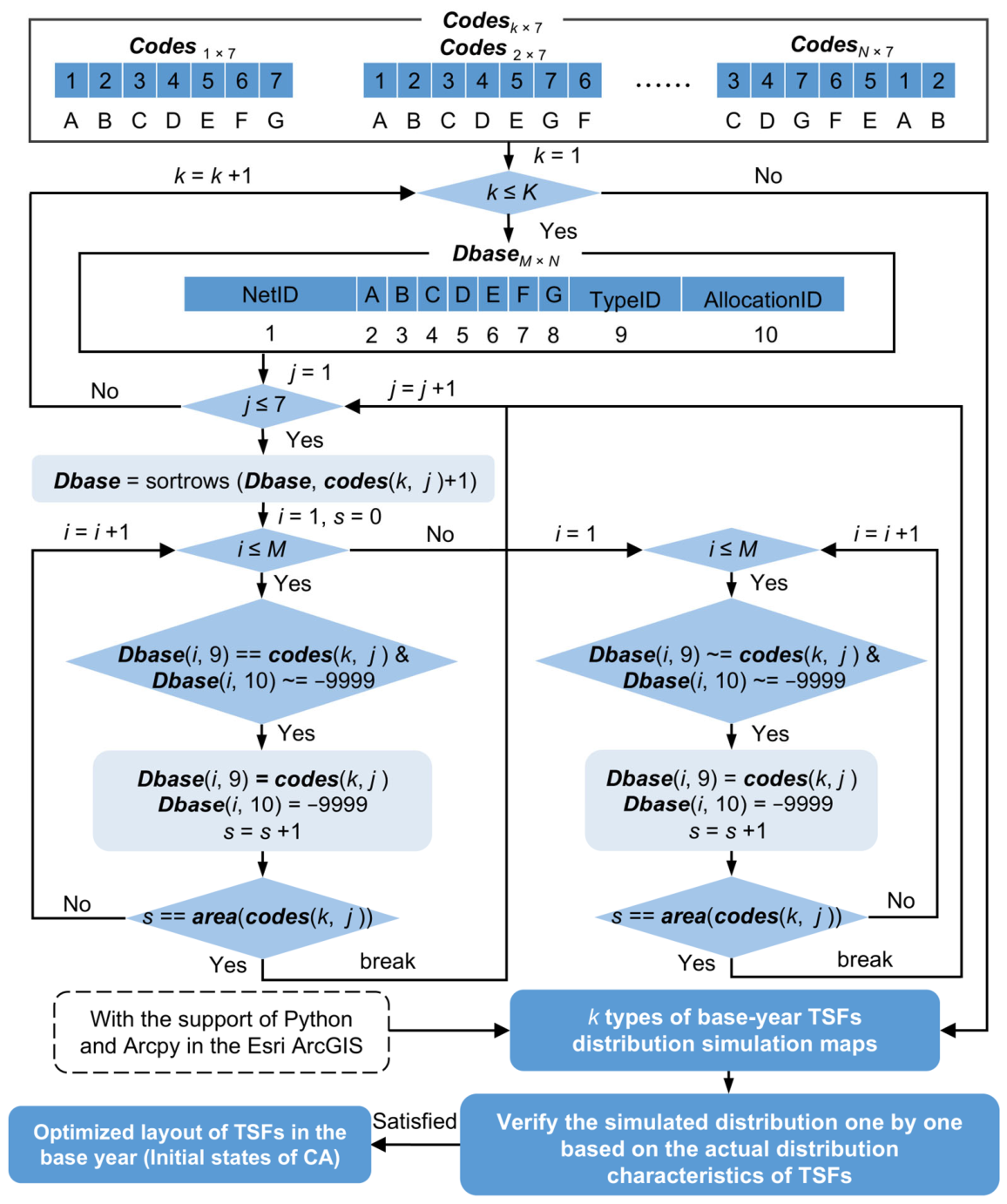
Based on the optimal area of TSFs in the baseline year (determined by Equation (9) in Section 3.2.1, subsection (3)), the coordinated suitability of TSFs (determined by Equation (10) in Section 3.2.2) and the steps for optimizing and adjusting TSFs (as described in Section 3.2.3), we designed an algorithm for obtaining the initial states of CA (Figure 4). We then used MATLAB and Python 3.11.8 to write the algorithm implementation program and obtained the optimal distribution of TSFs in the baseline year corresponding to the optimal scale of TSFs in 2025 and 2030 (refer to Figures S10 and S11 in the Supplementary Information, Section S10), and this was used as the initial state of CA.

4.3. Implementation of the TSFLO Model Solution

The solution steps of the TSFLO model are as follows. Step 1: Define each cell as a 50 m grid cell in the TSF distribution map. The cell state $S$ is one of the seven TSF types. UPF, ULF, RPF, RLF, EPSF, ERSF, and ESSF are coded as 1 through 7, respectively, so $S=\left\{1, 2, 3, 4, 5, 6, 7\right\}$, using a standard 5 × 5 neighborhood filter. Step 2: Use the baseline optimization of the TSF distribution raster maps corresponding to the years 2025 and 2030 (detailed acquisition methods are described in Section 4.2.3) as the initial states of the cellular space (Figures S10 and S11 in the Supplementary Information, Section S10). Step 3: Use the optimal transfer area matrices for TSFs from 2020 to 2025 and from 2020 to 2030 (detailed implementation steps are described in Section 4.2.1) as the cellular quantity conversion rules (Tables S7 and S8 in the Supplementary Information, Section S4). Step 4: Use the atlas of coordinated suitability for TSFs (detailed acquisition methods are described in Section 4.2.2) as the cellular space conversion rules (Figures S8 and S9 in the Supplementary Information, Section S9). Step 5: With the help of the CA–Markov tool in IDRISI software, the number of iterations was set to 5 and 10, and the tool was executed twice to obtain the results of the optimized configuration of the TSFL for coordinated low-carbon and economic growth in 2025 and 2030.

It should be noted that the optimizations for 2025 and 2030 both use 2020 as the common baseline year, but are solved independently using their respective target quantitative structures, Markov transition matrices, inverted CA initial states, and 5 and 10 iterations, respectively. The 2030 results were not obtained by continuing the evolution from the 2025 optimized layout as the initial state. Therefore, the difference in SFAR between the two target years reflects changes in the planning horizon and functional transition requirements, rather than a decline in the stability of the same model output under perturbations.

In the comparison between TSFLO and PLUS, both models used 50 m cells, a 5 × 5 neighborhood, the same baseline data, and the same target years, with 5 and 10 iterations applied for 2025 and 2030, respectively. These settings were fixed to establish a consistent basis for comparison at the same target year. This study did not test whether the outputs remained invariant under alternative spatial resolutions, neighborhood structures, or iteration settings; therefore, the relevant results were specific to the CA conditions specified in this study.

5. Results and Analysis

5.1. Layout Stability Analysis of TSFLO Model Optimization Results

5.1.1. Temporal Stability Analysis

In 2025, the SFAR of the layout generated by TSFLO was 81.40%, compared with 78.01% for PLUS, representing a difference of 3.39 percentage points. In 2030, the corresponding values were 73.60% and 73.32%, respectively, with TSFLO remaining 0.28 percentage points higher. Based on the total study area of 137,702 ha and a spatial resolution of 50 m, a difference of 0.28 percentage points corresponds to approximately 386 ha, or about 1540 spatial units. Therefore, TSFLO retained slightly more baseline functional units in both target years, with a more pronounced difference in 2025 and a smaller difference in 2030. SFAR represents the proportion of spatial units in which functional types remain unchanged in the optimized layout relative to the 2020 baseline layout; it reflects only the temporal retention of the layout and does not directly indicate the model’s ability to withstand external disturbances. The optimizations for 2025 and 2030 both started from the 2020 baseline but were solved independently using different target quantitative structures, Markov transition matrices, inverted CA initial states, and numbers of iterations. Accordingly, the decrease in SFAR from 81.40% to 73.60% for TSFLO and from 78.01% to 73.32% for PLUS reflects the longer planning horizon and changes in the target quantitative structures and functional transition requirements, and should not be used as a basis for comparing the relative performance of the two models. Model comparisons should be conducted for the same target year. On this basis, TSFLO had higher SFAR values than PLUS in both 2025 and 2030, although its relative advantage narrowed in 2030.

Whether the higher SFAR was attributable solely to the retention of baseline states also needs to be assessed in conjunction with quantitative coupling accuracy and spatial suitability results. The maximum absolute relative errors in the quantitative structure for TSFLO were 0.07% and 0.05% in 2025 and 2030, respectively, compared with 9.68% and 3.37% for PLUS. The minimum matching proportions between the seven functional types under TSFLO and their corresponding high-coordinated-suitability areas were 71.86% and 69.51% in 2025 and 2030, respectively, compared with 58.46% and 42.84% for PLUS. These results indicate that TSFLO not only achieved the target quantitative structure more accurately and maintained a higher degree of spatial suitability matching, but also retained more baseline functional units. Taken together, the SFAR and the above indicators support the conclusion that TSFLO exhibited better temporal stability in this case study, rather than suggesting that its higher SFAR was simply attributable to path dependence or system inertia.

5.1.2. Spatial Stability Analysis

The patch-level results showed that TSFLO exhibited lower MSI values for most functional types (Figure 5). In 2025, the MSI values of UPF, ULF, EPSF, ERSF, and ESSF under TSFLO were lower than those under PLUS. In 2030, the MSI values of UPF, ULF, RLF, EPSF, ERSF, and ESSF under TSFLO were lower than those under PLUS. This indicates that most functional patches generated by TSFLO had more regular shapes. The comparison results of PARA_MN showed no consistent pattern. In 2025, the PARA_MN values of RPF, RLF, and ESSF under TSFLO were lower than those under PLUS, whereas the values for the other functional types were higher. In 2030, the PARA_MN values of ULF, RPF, and ESSF under TSFLO were lower than those under PLUS, whereas the values for the remaining functional types were higher. Since lower PARA_MN values indicate shorter patch boundaries relative to patch area, higher PARA_MN values should not be interpreted as reduced fragmentation. Considering the two indicators together, TSFLO improved the regularity of patch shapes for most functional types, whereas its relative performance in terms of fragmentation varied across functional types and target years.

At the landscape scale, the relative performance of the two models varied with the target year and evaluation metric. In 2025, the CONTAG value of TSFLO was lower than that of PLUS. In 2030, the CONTAG values of TSFLO and PLUS were 47.70 and 46.85, respectively, with TSFLO being 1.82% higher, indicating that TSFLO generated more aggregated dominant patches and stronger landscape connectivity in this target year. The SHDI values of the two models were similar in both 2025 and 2030, suggesting comparable levels of patch-type diversity and area distribution evenness. Figure 6 illustrates the differences in local aggregation patterns between the two simulated layouts; however, it is not used to infer statistical significance. Therefore, TSFLO exhibited better aggregation and connectivity characteristics in 2030, whereas the CONTAG results in 2025 did not support the same conclusion.

Overall, when compared at the same target year, TSFLO exhibited a higher temporal retention ratio and lower MSI values for most functional types. However, its relative performance in terms of PARA_MN, CONTAG, and SHDI varied across functional types, evaluation metrics, and target years. Layout stability should be assessed jointly based on temporal retention, spatial pattern characteristics, quantitative coupling accuracy, and spatial suitability matching, and no single metric should be used to determine the overall conclusion independently. The current results support the relative advantages of TSFLO in terms of temporal stability and patch-shape regularity for most functional types, but do not indicate that it consistently outperforms PLUS across all spatial stability metrics, nor do they imply that the model outputs remain invariant under arbitrary changes in parameters.

5.2. Coupling Performance Analysis of the TSFLO Model Results

5.2.1. Quantitative Coupling Accuracy Analysis

The two models used the same baseline data and CA parameters; however, the resulting functional areas exhibited different degrees of deviation from the target-year optimal quantitative structure determined by MFLP (

Table 3. Quantitative coupling accuracy of the optimization results of the models.

TSFs	2025					2030
	MFLP	TSFLO		PLUS		MFLP	TSFLO		PLUS
	Area (ha)	Area (ha)	RE	Area (ha)	RE	Area (ha)	Area (ha)	RE	Area (ha)	RE
UPF	752.3	752.8	0.07%	752.3	0.00%	776.5	776.8	0.03%	776.5	0.00%
ULF	5878.8	5879.3	0.01%	5432.3	−7.60%	6534.8	6532.3	−0.04%	6534.8	0.00%
RPF	55,395.0	55,396.3	0.00%	55,395.0	0.00%	51,661.5	51,664.3	0.01%	53,247.3	3.07%
RLF	4752.3	4751.3	−0.02%	4752.3	0.00%	4260.3	4261.5	0.03%	4403.8	3.37%
EPSF	13,418.8	13,417.8	−0.01%	13,418.8	0.00%	16,758.0	16,756.5	−0.01%	16,758.0	0.00%
ERSF	52,892.8	52,892.0	0.00%	52,892.8	0.00%	53,098.0	53,100.3	0.00%	51,368.8	−3.26%
ESSF	4612.3	4612.8	0.01%	5058.8	9.68%	4613.0	4610.5	−0.05%	4613.0	0.00%

). In 2025, the relative errors of ULF and ESSF under the PLUS scenario were −7.60% and 9.68%, respectively, with a maximum absolute relative error of 9.68%. In 2030, the relative errors of RPF, RLF, and ERSF under the PLUS scenario were 3.07%, 3.37%, and −3.26%, respectively, with a maximum absolute relative error of 3.37%.

The quantitative structure obtained by TSFLO was closer to the MFLP-derived target values (Table 3). The maximum absolute relative errors in 2025 and 2030 were 0.07% and 0.05%, respectively, representing reductions of 99.28% and 98.52% compared with PLUS. Specifically, the areas of RPF and ERSF in 2025 and ERSF in 2030 were identical to the target values, while the deviations of the remaining functions did not exceed 0.07%. These differences directly indicate that TSFLO achieved higher quantitative coupling accuracy in this case study; they do not involve statistical significance testing.

TSFLO first estimates the target-year transition probability matrix (Figure 7) using the time-dependent functions of annual functional transition probabilities and then determines the optimal functional quantitative structure for the target year through MFLP. Subsequently, the model uses the Markov state-transition equation to inversely derive the baseline-year quantitative structure and transition area matrix (Figure 7) corresponding to the target quantitative structure, which are then used to construct the CA initial state and quantity transition rules, respectively. This linkage mechanism reduces the deviation between the CA-based spatial allocation results and the target quantitative structure, thereby improving the coupling accuracy between spatial layout and quantitative structure.

5.2.2. Spatial Coupling Performance Analysis

Spatial matching was evaluated using the proportion of each function located within areas of high coordinated suitability. For function $n$, this proportion was calculated as $r_n=S_{(p\ge v,n)}/A_n$, where $S_{(p\ge v,n)}$ represents the area of function $n$ distributed in regions with coordinated suitability equal to or higher than the threshold $v$, and $A_n$ represents the total area of function $n$. This metric directly measures the spatial consistency between the optimized layout and the corresponding high-coordinated-suitability areas of each function.

The lower panels of Figure 8 report the spatial matching proportions of the PLUS optimization results. In 2025, the matching proportions between the seven functional types and their respective high-coordinated-suitability areas ranged from 58.46% to 97.61%. In 2030, this range was 42.84% to 95.43%. These results indicate that the degree of spatial matching varied considerably among different functional types, and that some functions exhibited lower matching levels in 2030.

The TSFLO-derived layouts maintained relatively high matching proportions with high-coordinated-suitability areas (Figure 8). In 2025, the matching proportions of all seven functions were no lower than 71.86%. In 2030, the matching proportions of all functions remained above 69.51%. Compared with PLUS, TSFLO increased the minimum matching level, indicating that its spatial transition rules were more effective in allocating functions to their corresponding high-coordinated-suitability areas. This difference is associated with the use of game-theoretic selection probabilities in TSFLO to modify natural suitability and the construction of spatial transition rules based on coordinated suitability.

Figure 8. Spatial matching between the optimization results of the two models and coordinated suitability for territorial spatial functions. The upper panel shows the spatial overlay between the optimized layouts and high-coordinated-suitability areas, while the lower panel presents the matching area proportions of each function within high-coordinated-suitability areas.

Figure 8. Spatial matching between the optimization results of the two models and coordinated suitability for territorial spatial functions. The upper panel shows the spatial overlay between the optimized layouts and high-coordinated-suitability areas, while the lower panel presents the matching area proportions of each function within high-coordinated-suitability areas.

5.2.3. Analysis of Synergistic Effects

The decoupling state of the TSFL optimized by the PLUS model shows differentiated distribution characteristics for the periods 2020–2025 and 2020–2030 (

Table 4. Decoupling index of TSFL obtained from historical periods and model optimization.

TSFs	Historical Periods		TSFLO		PLUS
	2010–2020	2014–2020	2020–2025	2020–2030	2020–2025	2020–2030
UPF	0.6986	1.0494	0.0299	0.1032	0.0300	0.1032
ULF	0.2422	0.4359	0.3320	0.3826	0.4189	0.3827
RPF	0.1768	0.3756	0.9490	0.0162	0.9489	0.1002
RLF	0.3062	0.4007	0.5193	0.4795	0.5194	0.4573
EPSF	2.2014	−1.4612	−0.4242	−1.9341	−0.4240	−1.9351
ERSF	−0.1753	−0.4800	−1.7038	−2.8642	−1.7035	−1.9128
ESSF	0.2531	0.2482	0.4593	0.5194	0.5137	0.5191

). Specifically, UPF, ULF, RPF, RLF, and ESSF were in a state of weak decoupling in both periods, which indicates that the dependence of economic growth on carbon emissions decreased but still requires further optimization. EPSF and ERSF were in a strongly decoupled state in both periods, indicating that economic growth significantly outpaced carbon emissions growth, with good synergistic effects.

The decoupling types of the layouts generated by TSFLO and PLUS were generally similar, but substantial differences existed in the decoupling indices of some functions (Table 4). From 2020 to 2025, the decoupling index of ULF under TSFLO was 0.3320, which was lower than that under PLUS (0.4189); for ESSF, the values were 0.4593 and 0.5137, respectively. From 2020 to 2030, the decoupling index of RPF under TSFLO was 0.0162, lower than that under PLUS (0.1002); for ERSF, the values were −2.8642 and −1.9128, respectively. In contrast, when the functional areas allocated by the two models were nearly identical, their decoupling indices were also similar. For example, in 2030, the differences between the two models in the decoupling indices of UPF, ULF, EPSF, and ESSF were all small.

The two models used the same economic benefits and carbon emission coefficients per unit area for each function; therefore, differences in functional area allocation were the direct factor contributing to the above discrepancies. In 2025, the area of ULF allocated by TSFLO was 447.0 ha larger than that allocated by PLUS, whereas the area of ESSF was 446.0 ha smaller. In 2030, TSFLO allocated 1583.0 ha less RPF and 1731.5 ha more ERSF than PLUS. Differences in functional areas altered the total economic output and carbon emissions in the target years through the economic benefits and carbon emission coefficients per unit area of each function, thereby affecting the decoupling indices relative to 2020. These results explain the direct computational differences between the two models in this case study, but they cannot independently identify deeper causal drivers, such as industrial restructuring, technological progress, or policy implementation.

Compared with the historical periods (2010–2020 and 2014–2020), the TSFL optimized by both models demonstrated enhanced coordination of low-carbon and economic growth. During certain historical periods, the degree of decoupling of some functions fluctuated significantly. For example, the UPF index from 2014 to 2020 was 1.0494 (close to expansionary negative decoupling), suggesting that economic growth depended heavily on carbon emissions. The EPSF index from 2014 to 2020 was −1.4612 (strong decoupling), but with noticeable fluctuations. After model optimization, the decoupling indices of most functions (e.g., UPF, ULF, RLF, and ESSF) stabilized within the weak decoupling range. Those of strongly decoupled functions (EPSF, ERSF) further increased in absolute magnitude (e.g., the ERSF declined from −0.4800 to −2.8642). This indicates reduced dependence of carbon emissions on economic growth in the optimized spatial layout. However, constrained by the nonlinear coupling between carbon emissions and economic growth, and coupled with complex spatial interactions between carbon-sink and carbon-source functional zones, there remains significant potential for further improvement.

5.3. Optimized Layout of TSFs Using the TSFLO Model Under Different Case Scenarios

5.3.1. Quantitative Composition Analysis of Optimized Layouts

The results of the quantitative composition optimization of TSFs in Qionglai City in 2025 and 2030 are shown in

Table 5. Optimization results of the TSF quantitative composition in Qionglai City in 2025 and 2030.

TSFs		2020		2025		2030
First-Level	Second-Level	Area (ha)	%	Area (ha)	%	Area (ha)	%
Urban	UPF	621.81	0.45	752.80	0.55	776.80	0.56
	ULF	5226.56	3.80	5879.30	4.27	6532.30	4.74
Rural	RPF	62,483.97	45.38	55,396.30	40.23	51,664.30	37.52
	RLF	10,042.34	7.29	4751.30	3.45	4261.50	3.09
Ecological	EPSF	10,044.52	7.29	13,417.80	9.74	16,756.50	12.17
	ERSF	40,986.23	29.76	52,892.00	38.41	53,100.30	38.56
	ESSF	8296.58	6.03	4612.80	3.35	4610.50	3.35
Total		137,702	100	137,702	100	137,702	100

. In 2025, the areas for the urban, rural, and ecological spaces were modeled at 6632.10 hm², 60,147.60 hm², and 70,922.60 hm², constituting 4.82%, 43.68%, and 51.50% of the total area, respectively. Among the sub-categories, RPF space accounted for the largest share (40.23%), whereas UPF space accounted for the smallest share (0.55%). In 2030, the areas of urban, rural, and ecological spaces were modeled to reach 7309.10 hm², 55,925.80 hm², and 74,467.30 hm², constituting 5.31%, 40.61%, and 54.08% of the total area, respectively. Within the sub-categories, ERSF space became the largest (38.56%), whereas UPF space remained the smallest (0.56%).

Compared with the baseline year (2020), urban spaces in the target years 2025 and 2030 expanded by 783.73 hm² and 1460.73 hm², respectively, demonstrating incremental growth. This trend stems from the role of urban areas as commercial and industrial hubs that concentrate economic activities and populations. However, constrained by decelerating population growth, carbon emission reduction targets, and safeguard thresholds for food and ecological security, the pace of urban expansion has slowed. Rural spaces contracted by 12,378.71 hm² (in 2025) and 16,600.51 hm² (in 2030), indicating sustained reduction. This decline is driven by extensive local agricultural and livestock farming practices, resulting in inefficient land use and high carbon emissions. Additionally, the low level of intensive utilization of rural living spaces necessitates a transition to more efficient spatial use, leading to a reduction in the area of rural space. Meanwhile, ecological spaces increased by 11,595.27 hm² (in 2025) and 15,139.97 hm² (in 2030), reflecting consistent expansion. Such growth aligns with Qionglai City’s strategic positioning as a biodiversity conservation core zone and an ecological security barrier along the upper Yangtze River, thereby enhancing regional carbon sequestration capacity and ecosystem service functions.

Overall, under the constraints specified in this study, the target-year quantitative structure simultaneously addresses the objectives of economic growth, food security, ecological conservation, and carbon emission reduction by moderately increasing urban space, reducing rural space, and expanding ecological space. These quantitative adjustments are consistent with the optimization objectives and constraint directions defined for the case study; however, they do not demonstrate that the actual quantities of territorial spatial functions in the target years will change according to this scheme.

5.3.2. Spatial Layout Analysis of Optimized Layouts

The optimized TSFL in Qionglai City for 2025 and 2030 maintains the pattern of the baseline year (2020), demonstrating a consistent trend of urban agglomeration with efficiency gains, rural enhancement with scaled reduction, and ecological expansion with carbon sink augmentation (Figure 9). Specifically, UPF and ULF spaces consolidate in the central-eastern areas, forming a point–axis development system anchored by the towns of Linqiong, Yang’an, and Wolong. This aligns well with regional transportation networks and the distribution of industrial parks. This layout effectively improves the efficiency of the industrial division of labor and collaboration. It reduces additional carbon emissions caused by redundant facility construction and promotes the coordinated achievement of low-carbon and economic growth targets.

Rural areas are concentrated in the eastern plains and parts of the western region, with a dominant feature of a stable eastern region and a shrinking western region. RPF spaces are concentrated in townships such as Qianjin, Gaogeng, and Ranyi, as well as in the high-quality farmland in the western mountainous river valleys. RLF spaces are scattered across towns such as Ranyi, Yang’an, and Gaogeng, with a focus on relatively suitable living environments.

Ecological spaces are mainly distributed in the western mountainous regions and some areas of the southeast. Among these, EPSF spaces are concentrated in the central and western river valleys with well-preserved vegetation and water resources. ERSF spaces are predominantly distributed in western areas such as Tiantai Mountain, Gaohe, and Nanbaoshan Town, which are rich in flora and fauna and possess strong climate regulation and environmental purification capabilities. ESSF spaces are scattered across the southern regions of Tiantai Mountain, characterized by high biodiversity and excellent habitat quality. The newly designated ecological areas are located within the Longmen Mountains and the Nanhe River basin, ensuring the integrity of ecological corridors and enhancing carbon sequestration functions. This can offset part of the increased carbon emissions resulting from urban expansion, aligning with the objectives of regional ecological security barrier construction.

Overall, the functional spatial adjustments in 2025 and 2030 reflect differentiated allocation outcomes under the coordinated objectives of low-carbon development and economic growth. These results are used to illustrate the consistency of the optimized layouts with the objectives and spatial suitability conditions specified in this study and do not constitute predictive validation of the actual layouts in the target years.

6. Discussion

6.1. Methodological Extension of TSFLO and Its Technical Contributions

TSFLO is built upon established methods including MFLP, a non-homogeneous Markov process, game-theoretic models, and CA. Coupling MFLP with PLUS has been used to address target quantities and spatial allocation under uncertain conditions [7], while ESIUO has employed the Markov state-transition equation to inversely derive quantity transition rules and the CA initial state [13]. Game theory has also been combined with genetic optimization, CA, multi-criteria analysis, agent-based approaches, and linear programming [14,15,16]. Therefore, the contribution of TSFLO does not lie in any individual method or in their general combination. Rather, its contribution lies in the specific input–output relationships established among these modules and in the way functional conflict coordination participates in the construction of the CA initial state.

The quantity calculation starts from the optimal target-year quantitative structure $\mathit{X}$ obtained through MFLP. The non-homogeneous Markov process yields the cumulative transition probability matrix $\mathit{P}$ from the baseline year to the target year. Based on $\mathit{P}$, Equation (9) calculates ${\mathit{X}}^{\prime }={\left({\mathit{P}}^{\mathrm{T}}\right)}^{-1}\mathit{X}$, and Equation (8) further calculates $\mathit{x}=\mathrm{d}\mathrm{i}\mathrm{a}\mathrm{g}\left({\mathit{X}}^{\prime }\right)\mathit{P}$. ESIUO already incorporates a method for inversely deriving the baseline-year quantitative structure and quantity transition rules using the Markov state-transition equation [13]. Building on this approach, TSFLO transfers ${\mathit{X}}^{\mathrm{*}}$, obtained after accounting for parameter uncertainty through MFLP, into the inversion process, allowing the results of quantitative optimization to continue into the construction and iterative control of the CA initial state. Compared with the MFLP–PLUS model, which directly uses the results of quantitative optimization as demand parameters for PLUS [7], this process establishes an additional linkage among target-year quantities, baseline-year quantities, and CA quantity transition rules.

The spatial calculation starts from competition arising from multi-functional suitability. Existing game-theoretic models have mainly been used to coordinate land-use competition or describe strategic interactions among land developers, governments, and other actors [14,15,16]. TSFLO specifically uses a mixed-strategy Nash equilibrium to derive the functional selection probability ${\overline{x}}_{ki}$ of planning decision-makers and directly multiplies it by natural suitability $p_{ki}$ in Equation (10) to obtain coordinated suitability ${\rho }_{ki}$. This multiplicative adjustment does not introduce any additional weights. The game-theoretic results are thereby transformed into cell-level spatial allocation criteria and incorporated into the CA spatial transition rules.

During CA initial-state construction, ${\mathit{X}}^{\prime }$ specifies the target quantities that each function should attain in the baseline year, while ${\rho }_{ki}$ determines the order in which spatial units are adjusted. Section 3.2.3 enumerates the functional adjustment sequences and allocates spatial units in descending order of ${\rho }_{ki}$, thereby obtaining a baseline-year layout that satisfies ${\mathit{X}}^{\prime }$. This layout serves as the CA initial state, while $\mathit{x}$ and ${\rho }_{ki}$ continue to constrain subsequent quantity and spatial transitions. Compared with ESIUO, TSFLO retains the initial-state inversion approach, but extends the spatial basis for reconstructing the baseline-year layout from natural suitability to game-theoretic coordinated suitability, while the target quantities are obtained by MFLP under parameter uncertainty. Compared with existing MFLP–PLUS models and CA–game-theoretic models, TSFLO further links quantitative optimization, conflict coordination, and initial-state construction into a continuous computational process. This constitutes the methodological increment claimed by this study.

6.2. Strengths of the Model in Dealing with the Problem of the Synergistic Optimization of Low-Carbon and Economic Growth

In this study, layout stability refers to the extent to which, under the same target year and identical evaluation conditions, an optimized scenario responds to the target quantitative structure and spatial suitability requirements while maintaining continuity with the baseline functional layout and producing a relatively regular, connected, and not excessively fragmented spatial pattern. SFAR is used to characterize temporal retention relative to the 2020 baseline layout, whereas MSI, PARA_MN, CONTAG, and SHDI are used to characterize spatial pattern characteristics. SFAR alone cannot determine whether a higher retention ratio results from a reasonable continuation of the baseline layout or simply from maintaining the existing spatial pattern; therefore, it needs to be interpreted together with quantitative coupling accuracy and the matching degree with areas of high coordinated suitability. This concept differs from parameter robustness, which is assessed by changing external inputs and repeatedly running the model. MFLP is used to represent the uncertain ranges of parameters in quantitative optimization, where $\alpha$ is endogenously determined through the Bellman–Zadeh fuzzy decision-making process and the two-stage algorithm rather than being an externally specified sensitivity parameter [7,29,48]. The non-homogeneous Markov process is used to characterize the temporal variation in transition probabilities. The evaluation in this study compares the relative stability characteristics of the layouts generated by the two models under the given data conditions and evolutionary scenarios, rather than demonstrating that model outputs remain invariant under arbitrary changes in external inputs.

Existing integrated spatial optimization models can generate spatial layouts based on predefined quantitative demands; however, their approaches to handling key parameter uncertainty, functional conflicts, and the linkage with CA initial-state construction are different [9,13,14,15,16]. Many existing spatial optimization models have not sufficiently considered the impacts of key parameter uncertainty on spatial allocation processes [12]. Building on this limitation, TSFLO integrates MFLP, game-theoretic coordination, and the Markov state transition equation to address the corresponding issues in quantitative optimization, spatial transformation, and initial-state construction, respectively.

First, TSFLO addresses key parameter uncertainty during the quantitative optimization stage and transfers the optimized results to subsequent spatial allocation. The PLUS model can perform patch-level spatial allocation based on predefined target quantities; however, its core modules are not designed to estimate the uncertainty associated with external quantitative demands, benefit coefficients, and constraint thresholds [9,11]. TSFLO addresses this issue from two aspects. First, TSFLO represents the economic benefits per unit area, carbon emission coefficients, technical coefficients, and resource constraints as triangular fuzzy numbers within the MFLP framework and solves the resulting model using the Bellman–Zadeh fuzzy decision-making process and a two-stage algorithm [7,29,48]. In this process, $\alpha$ is the possibility level of the fuzzy parameters determined endogenously by the model, rather than a hyperparameter predefined by the researchers. In the first stage, the maximum objective satisfaction degree $\phi \left(\alpha \right)$ is obtained for each $\alpha$-cut within the range of $\alpha \in \left[\mathrm{0,1}\right]$, and the optimal possibility level $\alpha$ and the overall satisfaction degree $\rho$ are determined by maximizing $\rho \left(\alpha \right)=\mathrm{m}\mathrm{i}\mathrm{n}\left\{\alpha ,\phi \left(\alpha \right)\right\}$. In the second stage, $\alpha$ and $\rho$ are fixed, and the fully compensatory arithmetic mean satisfaction degree $\overline{\phi }=\left({\phi }_z+{\phi }_w\right)/2$ is maximized subject to the condition that the satisfaction degrees of both the benefit and cost objectives are no lower than $\rho$. This procedure determines a non-dominated quantitative structure $\mathit{X}$ that balances the low-carbon development and economic growth objectives from the acceptable solution set identified in the first stage. Rather than obtaining a specific result by manually selecting $\alpha$, this approach uses the two-stage algorithm to eliminate subjectivity in the selection of $\alpha$ and provides a determinate target quantitative structure for subsequent CA optimization.

Second, the model incorporates the coordination of TSFCs into functional layout optimization. Layout methods based on natural suitability often neglect the functional conflicts caused by multi-functional suitability and its spatial and temporal dynamics. This omission may reduce the consistency between the optimized layout and the evolving relationships among territorial spatial functions [60,61]. Our model breaks through this limitation from two aspects. First, to account for the spatiotemporal heterogeneity of functional transitions [62], we fitted differential equations to multi-year data on functional transition probabilities and used them to estimate the Markov transition probabilities for the target year. We incorporated these transition probabilities into the payoff matrix so that it represents the temporal dynamics of functional transitions and accounts for the non-stationarity of transition probabilities during spatial allocation. At the same time, the Nash equilibrium of the territorial spatial planner is used as the natural suitability correction coefficient. The coordinated suitability is then generated as the basis for the optimization for functional layout optimization. In game-theoretic terms, this Nash equilibrium indicates that neither player can increase its expected payoff by changing its strategy unilaterally under the specified payoff matrix and strategy spaces [63,64]. It provides the functional selection probabilities used to calculate coordinated suitability, but does not guarantee layout stability or demonstrate robustness to external disturbances. Secondly, the problem of negative solutions or no solution is prone to occur when a system of linear equations is applied to solve a zero-sum game (Tables S14 and S15 in Supplementary Information S11). We reformulated this problem as a constrained linear programming model and solved it using an interior-point method to obtain a feasible optimum satisfying the KKT conditions [65,66]. Meanwhile, the iteration tolerance of the interior-point method was set to 1.0 × 10⁻⁸ to control numerical error and verify the feasibility of the solution. The empirical comparison showed that the layout generated using coordinated suitability had greater temporal retention and more regular patch shapes for most functional types (Figure 10). These results support the assessment of relative layout stability under the conditions of this study, but do not establish resistance to external disturbances.

Third, our model improves the effect of coupling spatial layout, quantitative composition, and optimization objectives, thereby strengthening the rationality of the optimized TSF layout for coordinated low-carbon and economic growth. Models such as PLUS can perform spatial allocation under predefined quantitative demands; however, the treatment of uncertainty in quantitative parameters and the coordination of functional conflicts generally rely on external scenarios or additional models [9,11]. TSFLO further connects the target quantities derived from MFLP, the coordinated suitability generated through the game-theoretic model, and the CA initial state reconstructed through inversion for the baseline year, thereby enhancing the consistency of information transfer among spatial layout, quantitative structure, and optimization objectives. By contrast, the model proposed in our study addresses this issue in three aspects. First, based on the multi-year Markov transfer probability of TSF fitting differential equations, we can predict the probability of function transfers in the target year and establish Markov state transfer equations to solve the optimal quantity of functions in the target year corresponding to the optimal quantity of the base period year [13]. This addresses the disconnect between the functional quantity structure in the time dimension. Second, the game model amends the natural suitability of functions to a coordinated suitability as the basis for the adjustment of the functional layout in the baseline year [67]. The optimized layout of functions in the baseline year is obtained as the initial states of the CA. This enhances the dynamic adaptation of the layout to the functional conflict.

Figure 10. Comparison of the natural suitability, selection probability, and coordinated suitability of TSFs.

Figure 10. Comparison of the natural suitability, selection probability, and coordinated suitability of TSFs.

Fourth, we designed an exhaustive algorithm using MATLAB programming that calculates the layout scheme under multiple combinations of the functional adjustment order. Using the actual 2020 TSF layout shown in Figure S4 of Supplementary Information S7 as the reference, the algorithm excludes candidate layouts whose principal concentration areas, overall distribution directions, or basic spatial organization clearly depart from the baseline pattern. Candidate layouts consistent with the observed baseline distribution are retained as the CA initial states [68,69]. This enhances the rationality of the optimized layouts. The case study results show that the maximum absolute relative errors in the quantitative structure under TSFLO were 0.07% and 0.05% in 2025 and 2030, respectively, while the minimum matching proportions between the seven functional types and their corresponding high-coordinated-suitability areas were 71.86% and 69.51%, respectively. The SFAR values of TSFLO were higher than those of PLUS in both target years, and MSI values were also lower for most functional types. However, the relative performance of PARA_MN, CONTAG, and SHDI varied across functional types and target years. Therefore, the main advantages of TSFLO lie in the precise linkage between quantitative structure and spatial layout, the matching with areas of high coordinated suitability, and improvements in some layout stability metrics, rather than in a general advantage across all indicators.

6.3. Policy Implications

The policy implications of this study arise from the common spatial governance challenges faced by different countries and regions, rather than from the direct representativeness of Qionglai City for other areas. The IPCC Sixth Assessment Report identifies spatial planning, urban form, and infrastructure as important strategies for urban emission reduction [4]. Target 1 of the Kunming–Montreal Global Biodiversity Framework calls for integrated and biodiversity-inclusive spatial planning to reduce ecological losses caused by land-use change [5]. At the regional level, the African Union’s Agenda 2063 promotes inclusive growth and sustainable development, including the development of environmentally sustainable and climate-resilient economies and communities [70]. These policy priorities collectively require spatial decision-making approaches that coordinate economic development, emission reduction, and ecological conservation. TSFLO can translate these interconnected objectives into quantitative constraints and spatial allocation schemes, providing an analytical tool for comparing different policy scenarios.

First, territorial spatial optimization is an important way to alleviate the conflict between low-carbon and economic growth. Existing studies mostly focus on a single carbon emission reduction target. They ignore the relationship between low-carbon and economic growth. The TSFLO model achieves a spatial balance between development and conservation objectives by optimizing the spatial layout of production, living, and ecology by reducing the spatial proportion of high carbon emissions. This provides an alternative for developing countries to alleviate the pressure of high-cost and long-cycle emission reduction technology research and development.

Second, accounting for uncertainty in key parameters during TSF optimization provides an important basis for informed spatial governance. Conventional linear planning has limited capacity to address uncertainties brought about by socioeconomic changes in developing countries. TSFLO uses multi-objective fuzzy linear programming to represent uncertainty in key parameters during quantitative optimization. Policymakers can use the model to evaluate TSF allocation schemes under uncertain conditions and to support adaptive adjustments during plan implementation.

Third, a harmonious coexistence between humans and nature is the basic criterion for coordinating spatial conflicts. Traditional layouts based on natural suitability do not resolve functional conflicts and thus lack feasibility in practice. The TSFLO model integrates game theory, corrects the natural suitability of functions through the Nash equilibrium, clarifies the priority of functional development, and promotes sustainable development while mitigating conflicts. Developing countries need a balanced coexistence of human systems and natural systems throughout the entire course of spatial governance to realize a win–win situation between development and conservation.

Fourth, integrating spatial layout, quantitative composition, and optimization objectives can improve the internal consistency of territorial spatial planning and support its implementation. Existing models often neglect the synergy of these three, resulting in planning programs that are detached from reality. By integrating spatial layout, quantitative composition, and optimization objectives, TSFLO strengthens the consistency among these components and provides analytical support for implementing the optimized scheme. Planning authorities should examine whether these three components are properly aligned when formulating and implementing plans intended to coordinate economic development with environmental protection.

The above insights represent an analytical approach that can be recalibrated according to local conditions, rather than planning conclusions that can be directly replicated in other countries or regions. The Qionglai case only demonstrates the model’s performance under the data, 50 m analytical scale, fuzzy parameter ranges, functional transition patterns, and CA settings adopted in this study. When applying the model to other regions, parameter ranges, transition functions, spatial resolution, and CA settings need to be redefined according to local policy objectives, functional classifications, stakeholder relationships, and data conditions, and the resulting outputs need to be independently validated.

6.4. Limitations and Implications for Future Research

TSFLO integrates MFLP, a non-homogeneous Markov process, game-theoretic coordination, and CA initial-state inversion within the CA framework to improve consistency among spatial layout, quantitative composition, and optimization objectives. This integration provides a method for optimizing territorial spatial functional layouts while coordinating low-carbon development with economic growth. Nevertheless, this study has three limitations. First, the findings are conditional on the data, fuzzy parameter ranges, functional transition patterns, spatial resolution, and CA settings used in this study. The applicability of the model under other conditions remains to be established. Second, evidence from a single city cannot fully capture regional differences in resource and environmental conditions, development stages, or spatial governance arrangements. The findings therefore cannot be generalized directly to other regions. Third, TSFLO generates planning solutions under specified objectives and constraints, whereas their implementation outcomes may also be influenced by policy execution, stakeholder coordination, and socioeconomic change. These outcomes require further evaluation during implementation.

Future research should address these limitations in three areas. First, comparative studies under different data conditions, functional transition patterns, spatial scales, and model settings could clarify how these factors affect the optimization results and define the conditions under which the model can be applied. Second, applying TSFLO to regions with different resource and environmental conditions, development stages, and spatial governance arrangements would help identify regional differences in model structure and key parameters and support the development of region-specific calibration methods. Third, the planning implementation process could be incorporated into the evaluation framework. Continued monitoring of carbon emissions, economic growth, and changes in territorial spatial functions after implementation, together with information on policy execution, stakeholder participation, and compensation mechanisms, would allow planning outcomes to be evaluated and the model to be recalibrated accordingly.

7. Conclusions

This study develops the TSFLO model based on established methods, including MFLP, a non-homogeneous Markov process, a game-theoretic model, and CA initial-state inversion. The model transfers the optimal target-year quantitative structure obtained from MFLP to the Markov state-transition calculation and transforms the functional selection probabilities derived from the mixed-strategy Nash equilibrium into coordinated suitability. The optimal baseline-year quantitative structure and coordinated suitability are jointly used to construct the CA initial state, while the transition area matrix and coordinated suitability continue to constrain subsequent CA iterations. Through these mechanisms, the treatment of parameter uncertainty in quantitative optimization and functional conflict coordination are jointly propagated into the spatial allocation process, strengthening the linkage among spatial layout, quantitative structure, and the objectives of low-carbon development and economic growth.

Multi-objective fuzzy linear programming is used to address parameter uncertainty in the optimization of functional quantitative structures, while the game-theoretic model coordinates functional conflicts by modifying natural suitability; both components, together with CA initial-state inversion, contribute to territorial spatial function layout optimization. In comparisons conducted for the same target year, the SFAR values of TSFLO were 3.39 and 0.28 percentage points higher than those of PLUS in 2025 and 2030, respectively, indicating that TSFLO retained slightly more baseline functional units in both target years, although its relative advantage narrowed in 2030. The maximum absolute relative errors in the quantitative structure under TSFLO were 0.07% and 0.05% in 2025 and 2030, respectively, while the minimum matching proportions between the seven functional types and their corresponding high-coordinated-suitability areas were 71.86% and 69.51%, respectively. These results indicate that TSFLO retained more baseline functional units while achieving more accurate target quantitative structures and spatial suitability matching; therefore, its higher SFAR cannot be simply attributed to maintaining the existing layout. Because the results of the spatial pattern metrics varied across functional types and target years, the relative advantage of layout stability reported in this study is limited to temporal retention and patch-shape regularity for most functional types.

The TSFLO model uses Markov state transition equations combined with an MFLP-optimized target annual functional scale and differential-equation-predicted transition probabilities. In this way, it can simultaneously calculate the functional area transition matrix (i.e., cellular quantity transformation rules) and the baseline-year functional optimization area. By combining coordinated suitability to adjust the baseline-year functional layout, a functional distribution can be obtained that is consistent with the baseline-year functional optimization area (i.e., the initial states of CA). The CA initial state and the cellular quantity transformation rules derived using this method are combined with the cellular spatial transition rule based on coordinated suitability. Together, these components link spatial layout, quantitative structure, and optimization objectives within the CA framework. This linkage reduces functional conflicts and improves the rationality of multi-objective coordinated optimization. Our empirical evidence showed that the quantitative composition of the layout optimized by the TSFLO model had an error of ≤0.07% compared with the optimal target, and that the degree of conformity between each function and its high suitability zone was ≥70%. The dependence of economic growth on carbon emissions was reduced for some functions, such as the urban living function and rural production function, and the decoupling strength of ecological regulation functions increased by 49.7%, and the rationality of the TSFL was enhanced with improved coupling effects.

Overall, under the baseline data, 50 m spatial scale, fuzzy parameter ranges constructed in this study, and specified functional evolution scenarios for the Qionglai case, TSFLO performed well in terms of temporal retention, patch-shape regularity for most functional types, quantitative coupling accuracy, and spatial matching with areas of high coordinated suitability. MFLP, game-theoretic coordination, and CA initial-state inversion address parameter uncertainty in quantitative optimization, functional conflicts, and the linkage between spatial layout and quantitative structure, respectively, thereby providing decision support for territorial spatial function layout optimization under the coordinated objectives of low-carbon development and economic growth. These results do not imply that the model outputs remain invariant across all fuzzy parameter ranges, Markov transition scenarios, spatial resolutions, or CA settings, nor can the single Qionglai case demonstrate the empirical generalizability of the model across regions. When the model is applied to other regions, it needs to be recalibrated and validated according to local data and policy conditions. References [53,54,71,72,73,74,75,76,77,78,79,80,81,82,83,84,85,86,87,88,89,90,91,92,93,94,95,96,97,98,99,100,101,102,103,104,105] are cited in the reference list.

References

1. Jones, M.W.; Peters, G.P.; Gasser, T.; Andrew, R.M.; Schwingshackl, C.; Gütschow, J.; Houghton, R.A.; Friedlingstein, P.; Pongratz, J.; Le Quéré, C. National contributions to climate change due to historical emissions of carbon dioxide, methane, and nitrous oxide since 1850. Sci. Data 2023, 10, 155. [Google Scholar] [CrossRef] [Scilit] [PubMed]
2. Wang, S.; Zhou, L. Integrated impacts of climate change on glacier tourism. Adv. Clim. Change Res. 2019, 10, 71–79. [Google Scholar] [CrossRef] [Scilit]
3. Li, L.; Zhang, Y.; Zhou, T.; Wang, K.; Wang, C.; Wang, T.; Yuan, L.; An, K.; Zhou, C.; Lü, G. Mitigation of China’s carbon neutrality to global warming. Nat. Commun. 2022, 13, 5315. [Google Scholar] [CrossRef] [Scilit] [PubMed]
4. Lwasa, S.; Seto, K.C.; Bai, X.; Blanco, H.; Gurney, K.R.; Kılkış, Ş.; Lucon, O.; Murakami, J.; Pan, J.; Sharifi, A.; et al. Urban systems and other settlements. In Climate Change 2022: Mitigation of Climate Change. Contribution of Working Group III to the Sixth Assessment Report of the Intergovernmental Panel on Climate Change; Cambridge University Press: Cambridge, UK; New York, NY, USA, 2022; pp. 861–952. [Google Scholar] [CrossRef] [Scilit]
5. Conference of the Parties to the Convention on Biological Diversity. DECISION ADOPTED BY THE CONFERENCE OF THE PARTIES TO THE CONVENTION ON BIOLOGICAL DIVERSITY. In Proceedings of the Conference of the Parties to the Convention on Biological Diversity, Montreal, QC, Canada, 7–19 December 2022; Available online: https://www.cbd.int/doc/decisions/cop-15/cop-15-dec-04-en.pdf (accessed on 27 July 2026).
6. Zhang, K.; Liang, Q.-M. Recent progress of cooperation on climate mitigation: A bibliometric analysis. J. Clean. Prod. 2020, 277, 123495. [Google Scholar] [CrossRef] [Scilit]
7. Qin, J.; Ou, D.; Yang, Z.; Gao, X.; Zhong, Y.; Yang, W.; Wu, J.; Yang, Y.; Xia, J.; Liu, Y.; et al. Synergizing economic growth and carbon emission reduction in China: A path to coupling the MFLP and PLUS models for optimizing the territorial spatial functional pattern. Sci. Total Environ. 2024, 929, 171926. [Google Scholar] [CrossRef] [Scilit] [PubMed]
8. Hu, G.; Huang, J.; Shi, J.; Chen, S. The formation of the Chinese territorial spatial planning system and international comparison. Trans. Plan. Urban Res. 2023, 2, 16–36. [Google Scholar] [CrossRef] [Scilit]
9. Liang, X.; Guan, Q.; Clarke, K.C.; Liu, S.; Wang, B. Understanding the drivers of sustainable land expansion using a patch-generating land use simulation (PLUS) model: A case study in Wuhan, China. Comput. Environ. Urban Syst. 2021, 85, 101569. [Google Scholar] [CrossRef] [Scilit]
10. Verburg, P.H.; Soepboer, W.; Veldkamp, A.; Limpiada, R.; Espaldon, V.; Mastura, S.S.A. Modeling the Spatial Dynamics of Regional Land Use: The CLUE-S Model. Environ. Manag. 2002, 30, 391–405. [Google Scholar] [CrossRef] [Scilit] [PubMed]
11. Li, X.; Fu, J.; Jiang, D.; Lin, G.; Cao, C. Land use optimization in Ningbo City with a coupled GA and PLUS model. J. Clean. Prod. 2022, 375, 134004. [Google Scholar] [CrossRef] [Scilit]
12. Mehari, A.; Genovese, P.V. A Land Use Planning Literature Review: Literature Path, Planning Contexts, Optimization Methods, and Bibliometric Methods. Land 2023, 12, 1982. [Google Scholar] [CrossRef] [Scilit]
13. Ou, D.; Zhang, Q.; Tang, H.; Qin, J.; Yu, D.; Deng, O.; Gao, X.; Liu, T. Ecological spatial intensive use optimization modeling with framework of cellular automata for coordinating ecological protection and economic development. Sci. Total Environ. 2023, 857, 159319. [Google Scholar] [CrossRef] [Scilit] [PubMed]
14. Liu, Y.; Tang, W.; He, J.; Liu, Y.; Ai, T.; Liu, D. A land-use spatial optimization model based on genetic optimization and game theory. Comput. Environ. Urban Syst. 2015, 49, 1–14. [Google Scholar] [CrossRef] [Scilit]
15. Sadooghi, S.E.; Taleai, M.; Abolhasani, S. Simulation of urban growth scenarios using integration of multi-criteria analysis and game theory. Land Use Pol. 2022, 120, 106267. [Google Scholar] [CrossRef] [Scilit]
16. Hasti, F.; Salmanmahiny, A.; Rouhi, H.; Sakieh, Y.; Joolaei, R.; Pezhooli, N. Developing an integrated land allocation model based on linear programming and game theory. Environ. Monit. Assess. 2023, 195, 493. [Google Scholar] [CrossRef] [Scilit] [PubMed]
17. Cao, K.; Huang, B. Spatial optimization for land use planning: Opportunities and challenges. Trans. GIS 2019, 23, 641–644. [Google Scholar] [CrossRef] [Scilit]
18. Li, L.; Huang, X.; Yang, H. Optimizing land use patterns to improve the contribution of land use planning to carbon neutrality target. Land Use Pol. 2023, 135, 106959. [Google Scholar] [CrossRef] [Scilit]
19. Guo, Y.; Zhao, P.; Zhang, Y. Optimal allocation system of urban land use types under multi-objective constraints. Appl. Math. Nonlin. Sci. 2023, 9, 1–16. [Google Scholar] [CrossRef] [Scilit]
20. Dong, Y.; Liu, S.; Pei, X.; Wang, Y. Spatially explicit multi-objective optimization tool for green infrastructure planning based on InVEST and NSGA-II towards multifunctionality. Land Use Pol. 2025, 150, 107465. [Google Scholar] [CrossRef] [Scilit]
21. Ma, S.; He, J.; Liu, F.; Yu, Y. Land-use spatial optimization based on PSO algorithm. Geospat. Inf. Sci. 2011, 14, 54–61. [Google Scholar] [CrossRef] [Scilit]
22. Li, X.; Xu, H.; Ma, X.; Huang, Y. A two-step spatially explicit optimization approach of integrating ecosystem services (ES) into land use planning (LUP) to generate the optimally sustainable schemes. Land Degrad. Dev. 2023, 34, 2508–2522. [Google Scholar] [CrossRef] [Scilit]
23. He, Q.; Tan, S.; Yu, C.; Zhou, M. Collaborative optimization of rural residential land consolidation and urban construction land expansion: A case study of Huangpi in Wuhan, China. Comput. Environ. Urban Syst. 2019, 74, 218–228. [Google Scholar] [CrossRef] [Scilit]
24. Stewart, T.J.; Janssen, R.; Van Herwijnen, M. A genetic algorithm approach to multiobjective land use planning. Comput. Oper. Res. 2004, 31, 2293–2313. [Google Scholar] [CrossRef] [Scilit]
25. Masoomi, Z.; Mesgari, M.; Hamrah, M. Allocation of urban land uses by Multi-Objective Particle Swarm Optimization algorithm. Int. J. Geogr. Inf. Sci. 2013, 27, 542–566. [Google Scholar] [CrossRef] [Scilit]
26. Ma, C.; Zhou, M. A GIS-Based Interval Fuzzy Linear Programming for Optimal Land Resource Allocation at a City Scale. Soc. Indic. Res. 2018, 135, 143–166. [Google Scholar] [CrossRef] [Scilit]
27. Zhou, M. An interval fuzzy chance-constrained programming model for sustainable urban land-use planning and land use policy analysis. Land Use Pol. 2015, 42, 479–491. [Google Scholar] [CrossRef] [Scilit]
28. Zimmermann, H. Fuzzy programming and linear programming with several objective functions. Fuzzy Sets Syst. 1978, 1, 45–55. [Google Scholar] [CrossRef] [Scilit]
29. Lee, E.; Li, R. Fuzzy multiple objective programming and compromise programming with Pareto optimum. Fuzzy Sets Syst. 1993, 53, 275–288. [Google Scholar] [CrossRef] [Scilit]
30. Xu, T.; Gao, J.; Coco, G. Simulation of urban expansion via integrating artificial neural network with Markov chain—Cellular automata. Int. J. Geogr. Inf. Sci. 2019, 33, 1960–1983. [Google Scholar] [CrossRef] [Scilit]
31. Tong, X.; Feng, Y. A review of assessment methods for cellular automata models of land-use change and urban growth. Int. J. Geogr. Inf. Sci. 2020, 34, 866–898. [Google Scholar] [CrossRef] [Scilit]
32. Al-Sharif, A.; Pradhan, B. A novel approach for predicting the spatial patterns of urban expansion by combining the chi-squared automatic integration detection decision tree, Markov chain and cellular automata models in GIS. Geocarto Int. 2015, 30, 858–881. [Google Scholar] [CrossRef] [Scilit]
33. Yang, X.; Zheng, X.; Chen, R. A land use change model: Integrating landscape pattern indexes and Markov-CA. Ecol. Model. 2014, 283, 1–7. [Google Scholar] [CrossRef] [Scilit]
34. Wu, F. Calibration of stochastic cellular automata: The application to rural-urban land conversions. Int. J. Geogr. Inf. Sci. 2002, 16, 795–818. [Google Scholar] [CrossRef] [Scilit]
35. Krueger, J.I.; Heck, P.R.; Evans, A.M.; DiDonato, T.E. Social game theory: Preferences, perceptions, and choices. Eur. Rev. Soc. Psychol. 2020, 31, 222–253. [Google Scholar] [CrossRef] [Scilit]
36. Li, B.; Tan, G.; Chen, G. Generalized uncooperative planar game theory model for water distribution in transboundary rivers. Water Resour. Manag. 2016, 30, 225–241. [Google Scholar] [CrossRef] [Scilit]
37. Sheng, J.; Zhou, W.; Zhu, B. The coordination of stakeholder interests in environmental regulation: Lessons from China’s environmental regulation policies from the perspective of the evolutionary game theory. J. Clean. Prod. 2020, 249, 119385. [Google Scholar] [CrossRef] [Scilit]
38. Ghodsvali, M.; Dane, G.; de Vries, B. An integrated decision support system for the urban food-water-energy nexus: Methodology, modification, and model formulation. Comput. Environ. Urban Syst. 2023, 100, 101940. [Google Scholar] [CrossRef] [Scilit]
39. Wu, J.; Ge, Z.; Han, S.; Xing, L.; Zhu, M.; Zhang, J.; Liu, J. Impacts of agricultural industrial agglomeration on China’s agricultural energy efficiency: A spatial econometrics analysis. J. Clean. Prod. 2020, 260, 121011. [Google Scholar] [CrossRef] [Scilit]
40. Wu, Y.; Liu, Y.; Zeng, H. Ecosystem service supply–demand ratio zoning and thresholds of the key influencing factors in the Pearl River Delta, China. Landsc. Ecol. 2024, 39, 162. [Google Scholar] [CrossRef] [Scilit]
41. Li, S.; Zhao, X.; Pu, J.; Miao, P.; Wang, Q.; Tan, K. Optimize and control territorial spatial functional areas to improve the ecological stability and total environment in karst areas of Southwest China. Land Use Pol. 2021, 100, 104940. [Google Scholar] [CrossRef] [Scilit]
42. Huynh, L.T.M.; Gasparatos, A.; Su, J.; Dam Lam, R.; Grant, E.I.; Fukushi, K. Linking the nonmaterial dimensions of human-nature relations and human well-being through cultural ecosystem services. Sci. Adv. 2022, 8, 8042. [Google Scholar] [CrossRef] [Scilit] [PubMed]
43. Gu, Y.; Lin, N.; Ye, X.; Xu, M.; Qiu, J.; Zhang, K.; Zou, C.; Qiao, X.; Xu, D. Assessing the impacts of human disturbance on ecosystem services under multiple scenarios in karst areas of China: Insight from ecological conservation red lines effectiveness. Ecol. Indic. 2022, 142, 109202. [Google Scholar] [CrossRef] [Scilit]
44. Qu, Y.; Dong, X.; Su, D.; Jiang, G.; Ma, W. How to balance protection and development? A comprehensive analysis framework for territorial space utilization scale, function and pattern. J. Environ. Manag. 2023, 339, 117809. [Google Scholar] [CrossRef] [Scilit] [PubMed]
45. Ou, D.; Cheng, X.; Yan, Z.; Ruan, K.; Huang, Q.; Zhao, Z.; Yang, Z.; Qin, J.; Xia, J. Territorial functional pattern reconstruction integrating set-theoretic and functional mappings with game-theoretic analysis to reconcile development and conservation in China. Land 2025, 14, 2060. [Google Scholar] [CrossRef] [Scilit]
46. Zhu, W.; Lan, T.; Tang, L. Impacts of future climate change and xiamen’s territorial spatial planning on carbon storage and sequestration. Remote Sens. 2025, 17, 273. [Google Scholar] [CrossRef] [Scilit]
47. Sheng, P.; Li, J.; Zhai, M.; Majeed, M.U. Economic growth efficiency and carbon reduction efficiency in China: Coupling or decoupling. Energy Rep. 2021, 7, 289–299. [Google Scholar] [CrossRef] [Scilit]
48. Bellman, R.E.; Zadeh, L.A. Decision-making in a fuzzy environment. Manag. Sci. 1970, 17, B–141–B-273. [Google Scholar] [CrossRef] [Scilit]
49. Cococcioni, M.; Fiaschi, L.; Lambertini, L. Non-Archimedean zero-sum games. J. Comput. Appl. Math. 2021, 393, 113483. [Google Scholar] [CrossRef] [Scilit]
50. Jia, K.; He, H.; Zhang, H.; Guo, J. Optimization of territorial space pattern based on resources and environment carrying capacity and land suitability assessment. China Land Sci. 2020, 34, 43–51. [Google Scholar] [CrossRef]
51. Wang, Y.; Fan, J.; Zhou, K. Territorial function optimization regionalization based on the integration of “Double Evaluation. Geogr. Res. 2019, 38, 2415–2428. [Google Scholar] [CrossRef]
52. Ou, D.; Zhang, Q.; Qin, J.; Gong, S.; Wu, Y.; Zheng, Z.; Xia, J.; Bian, J.; Gao, X. Classification system for county-level territorial space using spatiotemporal heterogeneity and dynamic coupling of land use and functionality. Trans. Chin. Soc. Agric. Eng. 2021, 37, 284–296. [Google Scholar] [CrossRef]
53. Intergovernmental Panel on Climate Change. 2006 IPCC Guidelines for National Greenhouse Gas Inventories; Eggleston, H.S., Buendia, L., Miwa, K., Ngara, T., Tanabe, K., Eds.; IGES: Hayama, Japan, 2006. Available online: https://www.osti.gov/etdeweb/biblio/20880391 (accessed on 27 July 2026).
54. Intergovernmental Panel on Climate Change. 2019 Refinement to the 2006 IPCC Guidelines for National Greenhouse Gas Inventories; Calvo Buendia, E., Guendehou, S., Limmeechokchai, B., Pipatti, R., Rojas, Y., Sturgiss, R., Tanabe, K., Wirth, T., Romano, D., Witi, J., et al., Eds.; IPCC: Geneva, Switzerland, 2019; Available online: https://www.ipcc-nggip.iges.or.jp/public/2019rf/index.html (accessed on 27 July 2026).
55. Wang, X.; Ou, D.; Shu, C.; Liu, Y.; Yan, Z.; La, M.; Xia, J. How can we achieve carbon neutrality during urban expansion? An empirical study from Qionglai City, China. Land 2025, 14, 1689. [Google Scholar] [CrossRef] [Scilit]
56. Liu, H.C.; You, J.X.; You, X.Y.; Shan, M.M. A novel approach for failure mode and effects analysis using combination weighting and fuzzy VIKOR method. Appl. Soft Comput. 2015, 28, 579–588. [Google Scholar] [CrossRef] [Scilit]
57. Nie, F.; Zhang, P.; Li, J.; Ding, D. A novel generalized entropy and its application in image thresholding. Signal Process. 2017, 134, 23–34. [Google Scholar] [CrossRef] [Scilit]
58. Krejčí, J.; Stoklasa, J. Aggregation in the analytic hierarchy process: Why weighted geometric mean should be used instead of weighted arithmetic mean. Expert Syst. Appl. 2018, 114, 97–106. [Google Scholar] [CrossRef] [Scilit]
59. Chen, X.; Wang, D.; Chen, J.; Wang, C.; Shen, M. The mixed pixel effect in land surface phenology: A simulation study. Remote Sens. Environ. 2018, 211, 338–344. [Google Scholar] [CrossRef] [Scilit]
60. Zong, S.; Xu, S.; Huang, J.; Ren, Y.; Song, C. Distribution patterns and driving mechanisms of land use spatial conflicts: Empirical analysis from counties in China. Habitat Int. 2025, 156, 103268. [Google Scholar] [CrossRef] [Scilit]
61. Wang, P.; Zhang, L.; Lu, R.; Zhong, L. Multiscale territorial spatial conflict evolution and driving mechanism in China’s land border. Habitat Int. 2025, 156, 103302. [Google Scholar] [CrossRef] [Scilit]
62. Liu, X.; Li, X.; Yang, J.; Fan, H.; Zhang, J.; Zhang, Y. How to resolve the conflicts of urban functional space in planning: A perspective of urban moderate boundary. Ecol. Indic. 2022, 144, 109495. [Google Scholar] [CrossRef] [Scilit]
63. Nash, J.F. Equilibrium points in n-person games. Proc. Natl. Acad. Sci. USA 1950, 36, 48–49. [Google Scholar] [CrossRef] [Scilit] [PubMed]
64. Nash, J.F. Non-cooperative games. Ann. Math. 1951, 54, 286–295. [Google Scholar] [CrossRef] [Scilit]
65. Patterson, M.C. A linear programming model for solving complex 2-person zero-sum games. Stud. Econ. Financ. 1990, 13, 20–31. [Google Scholar] [CrossRef] [Scilit]
66. Pavlov, A.; Shames, I.; Manzie, C. Interior Point Differential Dynamic Programming. IEEE Trans. Control Syst. Technol. 2020, 29, 2720–2727. [Google Scholar] [CrossRef] [Scilit]
67. Paritosh, P.; Kalita, B.; Sharma, D. A game theory based land layout optimization of cities using genetic algorithm. Int. J. Manag. Sci. Eng. Manag. 2018, 14, 155–168. [Google Scholar] [CrossRef] [Scilit]
68. Zhang, Y.; Chang, X.; Liu, Y.; Lu, Y.; Wang, Y.; Liu, Y. Urban expansion simulation under constraint of multiple ecosystem services (MESs) based on cellular automata (CA)-Markov model: Scenario analysis and policy implications. Land Use Pol. 2021, 108, 105667. [Google Scholar] [CrossRef] [Scilit]
69. Ouyang, X.; Xu, J.; Li, J.; Wei, X.; Li, Y. Land space optimization of urban-agriculture-ecological functions in the Changsha-Zhuzhou-Xiangtan Urban Agglomeration, China. Land Use Pol. 2022, 117, 106112. [Google Scholar] [CrossRef] [Scilit]
70. Mkhize, S.; Ellis, D. Organic consumption as a means to achieve sustainable development goals and Agenda 2063. Sustain. Dev. 2024, 32, 5181–5192. [Google Scholar] [CrossRef] [Scilit]
71. Zhang, D.; Wang, W.; Zheng, H.; Ren, Z.; Zhai, C.; Tang, Z.; Shen, G.; He, X. Effects of urbanization intensity on forest structural-taxonomic attributes, landscape patterns and their associations in Changchun, Northeast China: Implications for urban green infrastructure planning. Ecol. Indic. 2017, 80, 286–296. [Google Scholar] [CrossRef] [Scilit]
72. Bai, L.; Tian, C.M.; Hong, C.H.; Kang, F.F.; Chen, J.Y.; Song, D.W.; Liu, H.G. The relationship between pine forest landscape patterns and pine wilt disease in Yichun, Hubei Province. Acta Ecol. Sin. 2015, 35, 8107–8116. [Google Scholar] [CrossRef] [Scilit]
73. Talukdar, S.; Eibek, K.U.; Akhter, S.; Ziaul, S.; Islam, A.R.M.T.; Mallick, J. Modeling fragmentation probability of land-use and land-cover using the bagging, random forest and random subspace in the Teesta River Basin, Bangladesh. Ecol. Indic. 2021, 126, 107612. [Google Scholar] [CrossRef] [Scilit]
74. Yang, W. Spatiotemporal change and driving forces of urban landscape pattern in Beijing. Acta Ecol. Sin. 2015, 35, 4357–4366. [Google Scholar] [CrossRef] [Scilit]
75. Wang, Q.; Wang, H. Spatiotemporal dynamics and evolution relationships between land-use/land cover change and landscape pattern in response to rapid urban sprawl process: A case study in Wuhan, China. Ecol. Eng. 2022, 182, 106716. [Google Scholar] [CrossRef] [Scilit]
76. Wang, D.M.; Yin, X.J.; Wang, J.J.; Gou, Z.Z.; Ma, A.Q.; Wu, P.J. Spatiotemporal evolution and driving forces of ecosystem health in the mountain-basin system on the northern slope of Tianshan Mountains. Geogr. Res. 2025, 44, 515–537. [Google Scholar] [CrossRef]
77. Špulerová, J.; Štefunková, D.; Kulcsár, C.; Kalivoda, H.; Vlachovičová, M.; Kočický, D. Development of indicators for assessment of green infrastructure for a territorial network of ecological stability. Biosyst. Divers. 2023, 31, 147–157. [Google Scholar] [CrossRef] [Scilit]
78. Weik, M.H. Computer Science and Communications Dictionary; Springer: New York, NY, USA, 2000. [Google Scholar] [CrossRef] [Scilit]
79. Shuai, C.; Chen, X.; Wu, Y.; Zhang, Y.; Tan, Y. A three-step strategy for decoupling economic growth from carbon emission: Empirical evidences from 133 countries. Sci. Total Environ. 2019, 646, 524–543. [Google Scholar] [CrossRef] [Scilit] [PubMed]
80. Wu, Y.; Chau, K.W.; Lu, W.; Shen, L.; Shuai, C.; Chen, J. Decoupling relationship between economic output and carbon emission in the Chinese construction industry. Environ. Impact Assess. Rev. 2018, 71, 60–69. [Google Scholar] [CrossRef] [Scilit]
81. Wang, Q.; Wang, S. A comparison of decomposition the decoupling carbon emissions from economic growth in transport sector of selected provinces in eastern, central and western China. J. Clean. Prod. 2019, 229, 570–581. [Google Scholar] [CrossRef] [Scilit]
82. Tapio, P. Towards a theory of decoupling: Degrees of decoupling in the EU and the case of road traffic in Finland between 1970 and 2001. Transp. Polic. 2005, 12, 137–151. [Google Scholar] [CrossRef] [Scilit]
83. Alhindawi, R.; Abu Nahleh, Y.; Kumar, A.; Shiwakoti, N. Projection of Greenhouse Gas Emissions for the Road Transport Sector Based on Multivariate Regression and the Double Exponential Smoothing Model. Sustainability 2020, 12, 9152. [Google Scholar] [CrossRef] [Scilit]
84. Sabri, R.; Tabash, M.I.; Rahrouh, M.; Alnaimat, B.H.; Ayubi, S.; AsadUllah, M. Prediction of macroeconomic variables of Pakistan: Combining classic and artificial network smoothing methods. J. Open Innov. Technol. Mark. Complex. 2023, 9, 100079. [Google Scholar] [CrossRef] [Scilit]
85. Ghysels, E.; Marcellino, M. Applied Economic Forecasting Using Time Series Methods; Oxford University Press: Oxford, UK, 2018; ISBN 9780190622015. [Google Scholar]
86. Lima, S.; Gonçalves, A.M.; Costa, M. Predictive accuracy of time series models applied to economic data: The European countries retail trade. J. Appl. Stat. 2023, 51, 1818–1841. [Google Scholar] [CrossRef] [Scilit] [PubMed]
87. Zhu, W.Q.; Pan, Y.Z.; Zhang, J.S. Estimation of net primary productivity of Chinese terrestrial vegetation based on remote sensing. Chin. J. Plant Ecol. 2007, 31, 413. [Google Scholar] [CrossRef] [Scilit]
88. Ou, D.; Zhang, Q.; Wu, Y.; Qin, J.; Xia, J.; Deng, O.; Gao, X.; Bian, J.; Gong, S. Construction of a Territorial Space Classification System Based on Spatiotemporal Heterogeneity of Land Use and Its Superior Territorial Space Functions and Their Dynamic Coupling: Case Study on Qionglai City of Sichuan Province, China. Int. J. Environ. Res. Public Health 2021, 18, 9052. [Google Scholar] [CrossRef] [Scilit] [PubMed]
89. Ganasri, B.P.; Ramesh, H. Assessment of soil erosion by RUSLE model using remote sensing and GIS-A case study of Nethravathi Basin. Geosci. Front. 2016, 7, 953–961. [Google Scholar] [CrossRef] [Scilit]
90. Chu, L.; Sun, T.; Wang, T.; Li, Z.; Cai, C. Evolution and Prediction of Landscape Pattern and Habitat Quality Based on CA-Markov and InVEST Model in Hubei Section of Three Gorges Reservoir Area (TGRA). Sustainability 2018, 10, 3854. [Google Scholar] [CrossRef] [Scilit]
91. Ma, S.; Wen, Z. Optimization of land use structure to balance economic benefits and ecosystem services under uncertainties: A case study in Wuhan, China. J. Clean. Prod. 2021, 311, 127537. [Google Scholar] [CrossRef] [Scilit]
92. Wang, Q.; Wang, S. Is energy transition promoting the decoupling economic growth from emission growth? Evidence from the 186 countries. J. Clean. Prod. 2020, 260, 120768. [Google Scholar] [CrossRef] [Scilit]
93. Wang, Q.; Su, M. The effects of urbanization and industrialization on decoupling economic growth from carbon emission–A case study of China. Sustain. Cities Soc. 2019, 51, 101758. [Google Scholar] [CrossRef] [Scilit]
94. Wu, Y.; Tam, V.W.Y.; Shuai, C.; Shen, L.; Zhang, Y.; Liao, S. Decoupling China’s economic growth from carbon emissions: Empirical studies from 30 Chinese provinces (2001–2015). Sci. Total Environ. 2019, 656, 576–588. [Google Scholar] [CrossRef] [Scilit] [PubMed]
95. Zhao, R.Q.; Huang, X.J.; Zhong, T.Y.; Cui, X.W. Carbon effect evaluation and low-carbon optimization of regional land use. J. Agric. Eng. 2013, 29, 220–229. [Google Scholar] [CrossRef]
96. Zhu, E.; Deng, J.; Zhou, M.; Gan, M.; Jiang, R.; Wang, K.; Shahtahmassebi, A. Carbon emissions induced by land-use and land-cover change from 1970 to 2010 in Zhejiang, China. Sci. Total Environ. 2019, 646, 930–939. [Google Scholar] [CrossRef] [Scilit] [PubMed]
97. Zhao, R.; Huang, X.; Liu, Y.; Zhong, T.; Ding, M.; Chuai, X. Carbon emission of regional land use and its decomposition analysis: Case study of Nanjing City, China. Chin. Geogr. Sci. 2015, 25, 198–212. [Google Scholar] [CrossRef] [Scilit]
98. Zhao, R.; Huang, X.; Peng, B. Research on carbon cycle and carbon balance of Nanjing urban system. Acta Geogr. Sin. 2012, 67, 758–770. [Google Scholar] [CrossRef]
99. Piao, S.; Fang, J.; Ciais, P.; Peylin, P.; Huang, Y.; Sitch, S.; Wang, T. The carbon balance of terrestrial ecosystems in China. Nature 2009, 458, 1009–1013. [Google Scholar] [CrossRef] [Scilit] [PubMed]
100. Shi, H.; Mu, X.; Zhang, Y.; Lv, M. Effects of different land use patterns on carbon emissions in Guangyuan City of Sichuan Province. Water Soil Conserv. Bull. 2012, 32, 101–106. [Google Scholar] [CrossRef]
101. Cai, Z.; Kang, G.; Tsuruta, H.; Mosier, A. Estimate of CH4 emissions from year-round flooded rice fields during the rice growing season in China. Pedosphere 2005, 15, 66–71. [Google Scholar]
102. He, Y.; Dan, L.; Dong, W.; Ji, J.; Qin, D. The terrestrial NPP simulations in China since the Last Glacial Maximum. Chin. Sci. Bull. 2005, 50, 2074–2079. [Google Scholar] [CrossRef] [Scilit]
103. Fang, J.; Guo, Z.; Pu, S.; Chen, A. Terrestrial vegetation carbon sinks in China, 1981–2000. Sci. China Ser. D 2007, 50, 1341–1350. [Google Scholar] [CrossRef] [Scilit]
104. Duan, X.N.; Wang, X.K.; Lu, F.; Ouyang, Z.Y. Carbon sequestration and its potential by wetland ecosystems in Chinas. Acta Ecol. Sin. 2008, 28, 463–469. [Google Scholar] [CrossRef]
105. Lai, L.; Huang, X.J.; Wang, H.; Dong, Y.H.; Xiao, S.S. Estimation of environmental costs of chemical fertilizer application in China. Acta Pedol. Sin. 2009, 46, 63–69. [Google Scholar] [CrossRef]
Figure 4. Flowchart of the algorithm used to obtain the optimal distribution of TSFs in the baseline year. c o d e s k × 7 is a k -row by 7-column array used to store the code combinations of various TSF types. E.g., c o d e s ( 1,1 ) = [ 1,2 , 3,4 , 5,6 , 7 ] denotes sequential adjustments to the spatial distribution of UPF (1), ULF (2), RPF (3), RLF (4), EPSF (5), ERSF (6), and ESSF (7). D b a s e M × N is an array with M rows and N columns, used to store spatial unit grid identifiers (NetID), suitability of the UPF(A), ULF(B), RPF(C), RLF(D), EPSF(E), ERSF(F), ESSF(G), TSF types (Type ID), and grid allocation identifiers (Allocation ID), where M represents the total number of spatial units. a r e a is a 1 by 7 array that respectively stores the optimal areas for UPF, ULF, RPF, RLF, EPSF, ERSF and ESSF. E.g., a r e a (1) represents the optimized area of UPF in the baseline year. s is a temporary variable used to store the optimized area of TSFs in the baseline year. 9999 indicates that the spatial unit has already been allocated to a certain type of TSF. i is the serial number of the spatial unit grid, where i = 1 ,   2 , . . .   , M . j is the column index of the c o d e s array, where j = 1,2 , . . .   , 7 . k is the serial number of the adjustment sequence combination of TSFs, where k = 1 ,   2 , . . . ,   K .
Sustainability 18 08920 g004
Figure 5. Landscape pattern indices of the optimization results of the models.
Sustainability 18 08920 g005
Figure 6. Comparison of the aggregation degree of model optimization results.
Sustainability 18 08920 g006
Figure 7. Matrices of TSF transition probability and area. (a,b) show the probability matrices of TSF transitions for the periods 2020–2025 and 2020–2030, respectively. (c,d) show the area matrices of TSF transitions for the periods 2020–2025 and 2020–2030, respectively.
Sustainability 18 08920 g007
Figure 9. Distribution of TSFs in the baseline year (2020) and optimization results of the TSFL in the target years (2025 and 2030).
Sustainability 18 08920 g009