Open Government Data, Resource Allocation Efficiency, and Sustainable Development in Manufacturing Firms: A Quasi-Natural Experiment Based on City-Level Government Data Platforms

Abstract

Open government data is a key institutional arrangement in market-oriented data factor reforms. Using the staggered rollout of city-level government data platforms in China as a quasi-natural experiment and panel data of listed manufacturing firms (2011–2024), we employ a staggered difference-in-differences design to examine the effect of open government data on firms’ resource allocation efficiency. We find that government data platforms significantly reduce resource misallocation, a result robust to propensity score matching, exclusion of concurrent policy shocks, and double machine learning. Channel-level tests do not find statistically significant transmission through government transparency, firm digital innovation, or fiscal subsidy reallocation. Directional identification shows that the effect operates primarily as a corrective force on capital-overallocated firms by curbing inefficient investment, rather than as a relief effect on constrained firms, and is more pronounced in high-digital-intensity industries, smaller cities, and regions with lower digital development. By reducing the wasteful use of capital, labour, and energy and improving the information environment in factor markets, open government data offers a low-cost, institutionalized instrument for reconciling productivity growth with sustainable resource use, with direct relevance to the United Nations (UN) Sustainable Development Goals (SDGs).

1. Introduction

The opening of government data has emerged as a key institutional arrangement in market-oriented reforms of data factors. In recent years, China has introduced a series of policies on data factors and digital government, prompting governments at various levels to launch public data platforms in phases and gradually consolidate and release data previously scattered across departments and administrative tiers. This institutional experiment raises an important empirical question: can government-led information disclosure genuinely improve resource allocation efficiency in markets? Existing research has accumulated findings along two relatively separate lines. Studies on open government data show that it enhances government transparency, fosters government–society interactions, and provides a data foundation for innovation [1,2,3]. Meanwhile, the resource misallocation literature documents that factor allocation distortions across firms are a major source of aggregate total factor productivity (TFP) losses in China’s manufacturing sector and that eliminating such misallocation could substantially raise TFP [4,5,6]. A small but growing literature has begun to connect these strands; Xu et al. [7] directly examine open government data and firm-level allocative efficiency, but the systematic quantification of allocative distortions within a structural framework and the decomposition of the direction of the policy effect remain to be developed.

Open government data may improve factor allocation by reducing information asymmetry and transaction costs. For firms, publicly available government data help identify market demand, understand local industrial policies and regulatory rules, and assess regional infrastructure and labour supply, thereby informing investment, production, and hiring decisions. For financial institutions, such data enhance their understanding of firms’ operational conditions and regional risks, improving the efficiency of credit evaluation. In the labour market, public information on government services, employment opportunities, and environmental quality shapes labour mobility and occupational choice. These channels suggest that open government data is not merely a governance reform but may systematically affect factor markets by reshaping the information environment. Prior literature has examined the role of digital technologies—such as digitization and data analytics capabilities—in promoting resource allocation [8,9,10]. Yet open government data, as a government-led data supply with strong externalities and broad coverage, may generate incremental effects beyond firms’ proprietary information systems. This possibility awaits rigorous empirical testing.

Building on these studies, we exploit the staggered rollout of city-level government data platforms in China as a quasi-natural experiment. Using panel data on listed manufacturing firms from 2011 to 2024, we employ a staggered difference-in-differences (DID) design to estimate the effect of open government data on firms’ resource allocation efficiency. Following the analytical framework of Hsieh and Klenow [4], we construct a firm-level measure of resource misallocation based on the deviation of a firm’s actual scale from its optimal scale. We find that the launch of government data platforms significantly reduces the degree of firm-level resource misallocation. This result is robust to propensity score matching, exclusion of concurrent policy shocks, and double machine learning. Channel-level tests do not find statistically significant transmission through government transparency, firm-level digital innovation, or the reallocation of fiscal subsidy resources. Analysis of the direction of the effect reveals that the policy primarily curbs inefficient investment by over-allocated firms rather than alleviating financing constraints faced by under-allocated firms. Heterogeneity analysis indicates that the effect is more pronounced in industries with high digital intensity, in smaller cities, and in regions with less developed digital economies, suggesting that open government data helps bridge the “digital divide.”

This paper makes three main contributions. First, building on the direct evidence in Xu et al. [7], we construct a firm-level measure of resource misallocation within the Hsieh–Klenow framework and provide causal evidence that open government data reduces allocative distortions, using a staggered DID design together with heterogeneity-robust estimators to address the bias of conventional two-way fixed effects under staggered adoption. Second, we decompose the average effect into a “corrective effect” on capital-overallocated firms and a significant worsening of allocative efficiency among expansion-needing firms, embedding the effective-investment channel documented by Wang et al. [11] within a full allocative-efficiency framework. Third, we systematically test three potential channels—governance transparency, digital innovation, and subsidy allocation—and report unsupported channels as such, and we provide formal heterogeneity tests of group differences. From a sustainability perspective, reducing factor misallocation limits the wasteful use of capital, labour, and energy inputs, so evidence on how data-governance institutions reshape factor allocation speaks directly to the sustainable development agenda (e.g., SDG 8 and SDG 12).

2. Institutional Background and Literature Review

2.1. Development and Current Status of Public Data Opening

Open government data refers to the practice by which governments and public agencies make publicly held data available through unified platforms in machine-readable and freely accessible forms [12]. This type of data possesses the dual nature of a public good and a quasi-public good: use by one firm does not deplete its value for others, yet the cost of accessing and processing it can exhibit partial excludability. Consequently, open government data cannot rely solely on market mechanisms and requires institutional design and government provision [13]. Unlike general information disclosure, which focuses primarily on transparency and the right to know, open government data places greater emphasis on machine readability, interoperability, and social value. This distinction reflects a shift from information accessibility to data usability—a shift that implies that the economic effects of open government data, particularly its impact on resource allocation in factor markets, should be regarded as a central dimension of policy evaluation.

China’s open government data policy has followed a gradualist path of bottom-up experimentation scaling from pilot projects to broader implementation. In 2015, the Action Outline for Promoting Big Data Development marked the first national-level exploration. In 2019, the Fourth Plenary Session of the 19th Central Committee formally recognized data as a factor of production alongside land, labour, capital, and technology, ushering in a new stage of market-oriented allocation of data factors. In 2022, Chinese authorities established a foundational institutional framework encompassing data property rights, circulation, and transaction mechanisms [14]. Within this policy context, local governments have progressively launched public data platforms, generating staggered temporal variation across cities—a key institutional resource for identifying the causal effects of open government data. By 2024, more than 200 prefecture-level cities and above in China had established government data platforms, although coverage remains uneven, with significantly higher adoption rates in eastern and central regions than in western and northeastern areas. From an international comparative perspective, China’s approach to open government data combines strong policy impetus and digital infrastructure advantages with latent shortcomings in data standardization, value realization, and property rights delineation [15]. Against this backdrop, the economic effects of open government data depend jointly on the scale of data supply and the diversity of user demand, providing an ideal setting for identifying its economic consequences from the perspective of resource allocation efficiency.

2.2. Literature Review

The resource misallocation literature provides a direct theoretical foundation for this study. Hsieh and Klenow, using firm-level data from China and India within a monopolistic competition framework, show that factor allocation distortions across firms can substantially reduce aggregate manufacturing total factor productivity [4]. Restuccia and Rogerson further characterize the sources of misallocation, including credit market frictions, tax preferences, and entry–exit barriers, which distort the firm size distribution and lower aggregate productivity. Building on the role of information frictions, David and Venkateswaran show through structural estimation that managers’ biased perceptions of productivity shocks are a key driver of factor misallocation–reducing information acquisition costs by 10 percent can raise aggregate TFP by approximately 2 percent [16]. Syverson, from an industrial organization perspective, notes that information frictions not only affect within-firm efficiency improvements but also reduce aggregate productivity by distorting the reallocation of resources across firms [17]. Together, these studies establish that information frictions serve as a critical micro-foundation of resource misallocation. Open government data, as an institutional arrangement that reduces the cost of information acquisition, holds the theoretical potential to improve resource allocation efficiency by alleviating these frictions.

Research on open government data has primarily focused on transparency, innovation, and public participation. Ubaldi [18] systematically reviews open data practices across OECD countries, emphasizing the synergistic effects of open frameworks, data interfaces, and government-society collaboration. Attard et al. [1] propose a lifecycle model for open data use, identifying data quality and standardization as key constraints on the effectiveness of open data initiatives. Janssen et al. [19] summarize barriers to open data use, noting that many datasets suffer from being available but unused. At the firm level, recent quasi-experimental studies based on China’s staggered government data platform launches have emerged. Wu et al. [20] find that platform launches increase firm-level TFP by approximately 4.5 percent. Li et al. [21] document an increase in firms’ employment scale following platform launches. Shan et al. [22] find that open government data improves firms’ labour investment efficiency and reduces incentives for firms to align with government preferences. Xu et al. [7] directly examine the link between open government data and resource allocation efficiency, finding that government data openness significantly improves firm-level allocative efficiency. Xu and Xu [23] document that government data platform launches significantly improve corporate ESG performance, providing additional evidence of the broad economic consequences of open government data.

Alongside this, information economics provides a more granular lens for understanding how open government data affects resource allocation. Classical models of markets with asymmetric information demonstrate that adverse selection caused by information asymmetry can force high-quality assets out of the market [24]. In factor markets, external investors lacking adequate information about firms’ true productivity cannot allocate capital to firms with the highest marginal returns. Goldfarb and Tucker argue that digitalization has substantially reduced search costs, replication costs, and verification costs, and that these reductions directly mitigate information asymmetries in capital markets [10]. In the Chinese context, Jiang and Li show, using listed firm data, that digital transformation improves the efficiency of capital allocation between firms by alleviating external information frictions. Moreover, the non-rival nature of data implies that the greater the degree of data sharing, the faster the social marginal returns accumulate. As an institutionalized data-sharing mechanism, open government data has distinct advantages over bilateral data transactions in lowering usage costs and expanding the scope of socialized use [25].

2.3. Literature Summary and Research Gap

Although the three strands of the literature—resource misallocation theory, open government data empirical research, and information economics—provide coherent points of intersection, empirical studies remain largely fragmented. The resource misallocation literature highlights the important roles of institutional distortions and information frictions but rarely engages with the possibility that proactive data-governance reforms could alleviate these frictions endogenously. The digital economy literature provides evidence that digitalization improves resource allocation efficiency, yet its focus is typically on firms’ own digital transformation rather than on the information public goods supplied by governments. Meanwhile, open government data research has largely remained at the level of transparency and innovation outcomes, with limited systematic analysis of factor market efficiency at the firm level. This paper builds on these studies by exploiting the staggered rollout of government data platforms for causal identification of the effect of open government data on firms’ resource allocation efficiency and by examining three potential channels—governance transparency, digital innovation, and fiscal subsidy allocation—to construct a more comprehensive analytical framework linking open government data to micro-level resource allocation.

Positioning relative to closely related studies. Three recent studies are especially close to ours. Xu et al. [7] use the staggered rollout of city-level government data platforms and find that open government data significantly improves firm-level allocative efficiency. Relative to that study, we construct the dependent variable directly within the Hsieh–Klenow framework as the deviation of each firm’s actual scale from its optimal scale, report a Goodman–Bacon decomposition and heterogeneity-robust estimators (Callaway–Sant’Anna, Borusyak–Jaravel–Spiess, and Sun–Abraham) to address the bias of two-way fixed effects under staggered adoption, and use directional classifications fixed at pre-treatment values to decompose the average effect into a corrective effect and a relief effect. Wang et al. [11] show that public data opening raises effective investment from the perspective of capacity utilization, which anticipates the corrective effect that we document. Relative to that study, we embed effective investment within a firm-level misallocation framework, estimate the effect on overall allocative efficiency, and formally distinguish the corrective effect from a relief effect. Wu et al. [20] focus on total factor productivity; allocative efficiency is a distinct margin, and our directional decomposition clarifies how the productivity gains operate.

3. Theoretical Framework and Research Hypotheses

3.1. Public Data Opening and Enterprise Resource Allocation Efficiency

Resource allocation efficiency refers to the degree to which factors of production achieve effective flow and matching across firms according to their marginal products. Prior research has repeatedly documented significant dispersion in capital and labour marginal products across firms in developing economies; reallocating output and factors across firms to reduce this dispersion could yield substantial aggregate TFP gains [4,26]. Consequently, any institutional arrangement that reduces information frictions or institutional transaction costs—thereby improving firms’ access to external information—can enhance resource allocation efficiency by narrowing the gap between factor prices and marginal products across firms. Open government data, as an institutional mechanism of this nature, can be systematically explained through several interrelated dimensions drawn from information economics.

From a search-theoretic perspective, firms face positive search costs when acquiring price information. The dispersion and acquisition cost of information mean that price dispersion for the same product across different markets persists over time, and this dispersion partly reflects resource allocation inefficiency arising from information asymmetry [27]. By releasing disaggregated industrial and market information through unified platforms, open government data systematically reduces firms’ information search costs across the entire economy, providing institutionalized information infrastructure for narrowing the dispersion of factor marginal products. When search costs decline, economic agents can compare expected returns across trading opportunities at lower information cost, and the dispersion of marginal products of capital and labour across firms correspondingly narrows, improving allocative efficiency.

From the economic properties of factors, the non-rival nature of data endows open government data with advantages over traditional information disclosure mechanisms. Jones and Tonetti demonstrate formally that because data can be used by one agent without reducing its availability to others, the repeated use and sharing of data can generate sustained productivity gains without incurring additional costs, implying that a social planner would choose significantly higher levels of data utilization than private markets would provide [25]. Open government data internalizes this externality through government intervention: data accumulated through administrative processes and standardized collection are released through open channels in machine-readable form, and any market participant can access and analyze these data for market assessment and investment decisions without incurring additional search costs. The non-rival nature—“opened once, used by many”—means that the improvement in resource allocation efficiency from open government data exhibits both amplification effects and scale effects.

From the structural transformation of information frictions in the digital era, Veldkamp argues that machine prediction technology is replacing traditional signal transmission and filtering mechanisms, thereby mitigating adverse selection and moral hazard caused by information asymmetry and fundamentally altering the allocation of capital and labour factors [28]. Within this framework, open government data provides all market participants with a shared, low-cost information platform that mitigates the “digital divide” and information inequality arising from disparities in data acquisition capabilities. Even small firms can access high-value external information at near-zero marginal cost and obtain a fairer competitive starting point in resource allocation. Crucially, the “public good” information provided by open government data forms a complementary relationship with firms’ internal data analytics capabilities. While firms’ internal data processing determines how effectively external data can be transformed into decision-relevant information, the richness of the external data supply amplifies the marginal returns of these internal capabilities, and the two forces jointly contribute to the improvement of factor allocative efficiency.

This theoretical logic has gained strong empirical support in the Chinese context; recent quasi-experimental studies exploiting the same platform rollout document improvements in productivity, financing costs, investment efficiency, and cross-regional capital flows (Section 2.2). These findings jointly point to a coherent inference: when governments release high-quality, widely applicable public data in an institutionalized form, firms can identify high-return opportunities at lower information cost and make more efficient investment decisions, while external monitors can exercise oversight with greater transparency, reducing the cost of due diligence. Based on this, the gap between firm-level factor marginal products narrows, and resource allocation efficiency improves.

Hypothesis 1 (H1). 

Open government data can significantly improve firms’ resource allocation efficiency.

3.2. Government Governance Transparency Channel

Government governance transparency is an important institutional factor affecting micro-level economic agents. As a core component of governance transparency, fiscal transparency directly determines the quality and quantity of information available to firms, investors, and the public regarding government operations. When fiscal information flows without obstruction, firms can more accurately assess policy direction, business environment risks, and the orientation of public resource allocation, thereby making more efficient investment and operational decisions [29,30].

The launch of government data platforms constitutes a systematic reform of public information disclosure. By releasing structured data across multiple dimensions—fiscal budgets, approval portals, and public resource allocation—through unified open platforms, these initiatives directly reduce the cost for firms to access market-related information, and through the signalling effect of proactive data disclosure, they demonstrate the government’s commitment to transparency and accountability. From the perspective of information economics, increased governance transparency affects resource allocation efficiency through two pathways. First, it reduces information search costs. When fiscal budget and spending information is published in standardized, comparable form in a timely manner, firms and investors can analyze regional fiscal conditions, industry support priorities, and infrastructure development at a lower cost, thereby mitigating the adverse selection and resource misallocation that arise from information scarcity [27]. Second, it strengthens external monitoring and accountability. Greater fiscal transparency increases the observability of government behaviour, enabling the public and auditing institutions to more effectively identify inefficiencies and rent-seeking in the use of public funds. This monitoring effect imposes constraints and incentives on the process of public resource allocation, prompting governments to prioritize efficiency and equity when allocating fiscal resources [31].

Critically, improvements in governance transparency can generate a virtuous cycle. When local governments make progress in open government data and fiscal information transparency, the information asymmetry between governments and firms is reduced, and the signalling mechanism strengthens market confidence in the region’s business environment. These positive expectations are ultimately reflected in the pricing efficiency of capital markets: when information and governance transparency improve, both firms’ financing costs and valuation biases decrease, and capital flows more closely align with real efficiency.

Hypothesis 2 (H2). 

Open government data improves firms’ resource allocation efficiency by enhancing government governance transparency.

3.3. Digital Innovation Empowerment Channel

Digital technology serves as a critical micro-level mechanism driving the optimization of firm resource allocation. A growing body of research shows that digital transformation and innovation at the firm level can significantly improve resource allocation efficiency. Dupor et al. [32] find that information technology adoption reshapes firm growth dynamics, while Baba-Yara et al. [33] show that artificial-intelligence-related investments significantly drive firm expansion and industry concentration. Jiang and Li find that the higher a firm’s degree of digitalization, the greater its capital and labour allocation efficiency [8]. Wu and colleagues construct a firm-level resource allocation index and find that digital transformation significantly reduces the degree of resource misallocation [34]. Ding and colleagues show that firms with higher digitalization experience a greater decline in resource misallocation, with reductions in information asymmetry and improvements in technological capabilities serving as key channels [35]. Yang uses annual report text to construct a digital transformation index and finds that digitalization improves capital allocation, with information asymmetry reduction identified as a critical pathway [36].

Building on this literature, firm-level digital innovation can be understood as the specific, observable dimension through which digital transformation affects resource allocation efficiency. Unlike passive digital input adoption, digital innovation involves the application of digital technologies across the entire value chain—product design, production processes, and business models. When firms possess digital technology and data analysis capabilities, they can embed data-driven decision-making into product development, customer screening, supply chain management, and risk control. On the product side, firms can identify higher-value niche markets and allocate research and development (R&D) resources to new segments; on the production side, firms can optimize processes and capacity arrangements to reduce the inefficient occupation of capital by excess capacity [37]. Digital innovation is not limited to hardware investment; by transforming information collection processes and decision-making rules, it converts dispersed, tacit knowledge into computable, predictable signals, guiding resource allocation closer to the direction of true marginal returns [9].

Open government data provides essential “raw materials” for firm-level digital innovation. Government data platforms, by releasing urban economic and social data at low or zero marginal cost, enrich the information dimensions available to firms—including market segmentation, industry policy dynamics, consumer trends, and risk alerts. When firms possess the corresponding data analysis capabilities, they can integrate these external data with their internal operational information, driving digital innovation in products, processes, and business models. Case studies by Jetzek and colleagues demonstrate that products and services built on open government data generate significant economic value through data-driven innovation [38]. Wang and Hu, using Chinese listed firm data, find that the launch of local government data platforms significantly increases firms’ open innovation levels [39]. Wang et al. [40] similarly find that public data elements significantly drive enterprise digital transformation, particularly through enhanced data-driven innovation capabilities. Sun and colleagues show that open government data promotes corporate innovation capacity, with the primary mechanism being the mitigation of information asymmetry that enables firms to identify market opportunities and technology trends more accurately, thereby enhancing R&D and innovation output [41].

Within this causal chain, digital patent applications serve as the most direct and credible measure of firm-level digital innovation output. Patents undergo substantive examination through intellectual property review and thus carry higher innovation content and technical credibility, effectively reflecting substantive rather than superficial innovation. Following the opening of government data, firms can access external information at lower cost and integrate it with internal R&D to promote the filing of digital technology patents. By improving firms’ digital innovation capacity, open government data optimizes factor allocation and thereby enhances resource allocation efficiency.

Hypothesis 3 (H3). 

Open government data improves firms’ resource allocation efficiency by enhancing their digital innovation capacity.

3.4. Subsidy Resource Allocation Optimization Channel

The allocation of fiscal subsidies across firms directly shapes the direction of resource flow among firms with different productivity levels. Prior studies have shown that when governments subsidize inefficient firms, they inflate inefficient capacity while crowding out the market space of efficient firms, exacerbating the misallocation of capital and labour across firms [42,43]. The theory of soft budget constraints further argues that when governments provide loss-making firms with tax reductions, subsidies, or administrative relief, the cost and risk discipline faced by inefficient firms is weakened, allowing them to continue operating through external transfusions rather than organic growth, ultimately forming zombie firm clusters [44,45]. Branstetter and colleagues document through empirical analysis that subsidies to Chinese listed firms are significantly associated with firm size but do not systematically flow to more productive firms [46]. Such subsidy bias traps resource allocation in long-term inefficiency.

Open government data provides the institutional conditions for changing the subsidy allocation process through improved governance transparency. When fiscal information becomes transparent, the funding status and performance outcomes of subsidized firms and projects are more easily observed by the public, media, and higher-level regulatory authorities. Local governments cannot easily continue to allocate subsidies to the same inefficient recipients solely on the basis of private information or relational ties, but must instead justify their allocation decisions under greater public scrutiny [29]. Subsidizing inefficient or zombie firms imposes higher reputational and political costs, since the information is publicly visible. By contrast, limited fiscal resources are more likely to flow toward firms with strong growth potential and clearly specified development directions, as their policy alignment and expected returns are easier to justify and are less likely to trigger negative public feedback. Transparency thus changes the cost structure of subsidy allocation, prompting local governments to incorporate efficiency and innovation performance into their allocation criteria.

At the empirical level, this mechanism can be characterized from two analytical perspectives. First, from the perspective of allocative efficiency, if open government data genuinely alters the process of subsidy allocation, subsidies should become more responsive to firms’ innovation performance following the data platform launch. This can be tested by examining whether the association between firm innovation and subsidies strengthens after the launch. Second, from the perspective of structural changes in subsidy intensity, if open government data improves information transparency, firms with higher R&D intensity should receive increased subsidy intensity following the platform launch. This can be tested through an interaction term between R&D intensity and the DID treatment indicator. Taken together, when governments release high-quality public data in an institutionalized form, firms’ subsidy allocation shifts from a “relationship-based” or “size-based” logic toward a “capability-efficiency” logic, and the strengthening of the subsidy–innovation linkage—along with the restructuring of subsidy allocation—directs scarce fiscal resources toward firms with higher productivity and innovation efficiency, thereby reducing the degree of resource misallocation.

Hypothesis 4 (H4). 

Open government data improves firms’ resource allocation efficiency by optimizing subsidy allocation structures, reflected in a stronger responsiveness of subsidy allocation to firm innovation.

4. Research Design

4.1. Model Construction

To test the effect of open government data on firms’ resource allocation efficiency, we treat the staggered rollout of government data platforms as a quasi-natural experiment and specify a two-way fixed effects staggered difference-in-differences model:

$$Misallo{c}_{it}=\alpha +\beta D_{c\left(i\right),t}+\gamma contro{l}_{it}+{\mu }_i+{\lambda }_t+{\epsilon }_{it}$$

(1)

where $Misallo{c}_{it}$ is the dependent variable representing the resource allocation efficiency of firm i in year t, measured in levels (not logarithms) as described in Section 4.2.1; $D_{c\left(i\right),t}$ is the core explanatory variable, which takes the value of 1 if the firm’s city $c\left(i\right)$ has launched a government data platform in year t and 0 otherwise. $\beta$ is the coefficient of interest, capturing the average treatment effect of open government data on firms’ resource allocation efficiency. $control$ is a vector of control variables with coefficient vector $\gamma$; $\alpha$ is the intercept; ${\mu }_i$ represents firm fixed effects; ${\lambda }_t$ represents year fixed effects; and ${\epsilon }_{it}$ is the idiosyncratic error term.

4.2. Variable Selection

4.2.1. Explained Variable

The dependent variable in this study is manufacturing firms’ resource allocation efficiency. Hsieh and Klenow [4] examine aggregate efficiency losses by analyzing output distortion and capital distortion at the firm level. Building on their framework, Wei and colleagues further develop a firm-level indicator system that measures resource allocation efficiency by quantifying the gap between a firm’s optimal scale and its actual scale under the assumption that all firms within an industry face the same underlying production technology [47]. Following this approach with appropriate extensions and refinements, our model specification is as follows.

Under the theoretical framework, suppose each firm within the same industry faces similar production technology at a given time. The industry production function takes the constant-returns-to-scale Cobb–Douglas form:

$$Y_{ist}=A_{st}{K}_{ist}^{{\alpha }_{st}}{L}_{ist}^{1-{\alpha }_{st}}$$

(2)

where $Y_{ist}$ is the real output of firm i in industry s in year t, measured by industrial value added (operating revenue minus intermediate inputs plus VAT payable). Price deflators are applied using provincial industrial product ex-factory price indices, fixed asset investment price indices, and consumer price indices, with 2012 as the base year. Intermediate inputs are calculated as operating costs plus selling expenses, administrative expenses, and financial expenses minus cash paid to and for employees, fixed asset depreciation, and amortization. Since listed firms do not directly disclose VAT payable, we follow the estimation approach of Yu [48]: estimated VAT payable = (cash received from sales of goods and services − cash paid for purchases of goods and services)/(1 + VAT rate) × VAT rate, where the VAT rate follows the statutory general rate of 17% during 2011–2017, 16% in 2018, and 13% from 2019 onward. $A_{st}$ is total factor productivity of industry s in year t; $K_{ist}$ is capital input, measured by net fixed assets; $L_{ist}$ is labour input, using cash paid to and for employees as a proxy for labour compensation. ${\alpha }_{st}$ is the capital elasticity, assumed to be constant across firms within the same industry, such that observable differences in output come primarily from factor distortions rather than technology differences. Parameters are estimated by regression under the Cobb–Douglas specification.

Taking logarithms yields the estimating equation:

$$\ln Y_{ist}={\beta }_{0,st}+{\beta }_{K,st}\ln K_{ist}+{\beta }_{L,st}\ln L_{ist}+{\epsilon }_{ist}$$

(3)

where ${\epsilon }_{ist}$ captures unobserved firm-level technology differences. Under constant returns to scale, the capital elasticity is obtained from the coefficient estimates:

$${\alpha }_{st}={\displaystyle \frac{{\beta }_{K,st}}{{\beta }_{K,st}+{\beta }_{L,st}}}$$

(4)

where ${\beta }_{K,st}$ and ${\beta }_{L,st}$ represent the marginal contributions of capital and labour inputs, respectively, and their sum is the total output elasticity.

To address the issue of insufficient firm observations in some industry–year cells, we apply the method of iterative estimation. If a specific industry–year cell has too few observations, the industry’s all-period average ${\alpha }_s$ is used. If the all-period estimate remains unavailable, the economy-wide weighted average ${\alpha }^{all}$ is applied:

$${\alpha }^{all}=\sum _s{w}_s{\alpha }_s,w_s={\displaystyle \frac{{\sum }_{i,t}{Y}_{ist}}{{\sum }_{s,i,t}{Y}_{ist}}}$$

(5)

where $w_s$ is the output weight of industry s, reflecting its relative importance. This weighting scheme mitigates the influence of small-sample estimation bias. To ensure comparability across years, all nominal variables are deflated to 2012 constant prices:

$$X_{ist}={\displaystyle \frac{P_{ist}}{D_{p,t}/D_p}}$$

(6)

where $X_{ist}$ is the real variable, $P_{ist}$ the nominal value, and $D_{p,t}$ the price index for province p in year t (output is deflated using the industrial product ex-factory price index, capital using the fixed asset investment price index, and labour using the consumer price index, with $D_p=1$ for 2012). To reduce the influence of outliers on regression estimates, $Y_{ist}$, $K_{ist}$, and $L_{ist}$ are winsorized at the 1% and 99% levels.

Under perfect competition, firms’ factor returns equal their marginal products. However, in the presence of policy distortions and market frictions, the effective prices faced by firms deviate from their efficient levels. Following Hsieh and Klenow [4], the output distortion and capital distortion for firm i in industry s are defined as

$$1-{\tau }_{Y,ist}={\displaystyle \frac{\omega L_{ist}}{(1-{\alpha }_{st})Y_{ist}}},1+{\tau }_{K,ist}={\displaystyle \frac{{\alpha }_{st}{Y}_{ist}}{K_{ist}}}·{\displaystyle \frac{1-{\tau }_{Y,ist}}{R}}$$

(7)

where ${\tau }_{Y,ist}$ captures the output market distortion, ${\tau }_{K,ist}$ captures the capital market distortion, $\omega$ is the labour price, and R is the capital return. We normalize $\omega =1$ and set $R=0.1$, implying an annual capital return of approximately 10%. Because labour input is measured as real cash payments to employees, i.e., the labour compensation of the firm, the wage parameter $\omega$ serves as a units normalization rather than an assumption that wages are equal across firms or regions. In this measurement, $L_{ist}$ already incorporates regional differences in wage levels: a firm with the same employment in a higher-wage region has proportionally larger labour compensation. Consequently, alternative province- or firm-specific wage calibrations that preserve the identity ${\omega }_{ist}{L}_{ist}=$ labour compensation leave the constructed distortion measures unchanged. The first expression in Equation (7) reflects deviations in labour allocation: when the effective price of labour is distorted downward, $(1-{\tau }_Y)$ is smaller. The second expression captures deviations in capital allocation: when the effective cost of capital is distorted upward, $(1+{\tau }_K)$ is larger. Together, these two terms characterize the overall level of firm-level distortions.

When firms face no distortions, actual output equals its optimal level. Following Hsieh and Klenow’s derivation, the ratio of optimal output to actual output is

$${\displaystyle \frac{Y_{ist}^{opt}}{Y_{ist}}}={(1-{\tau }_{Y,ist})}^{-(\sigma -1)}{(1+{\tau }_{K,ist})}^{-{\alpha }_{st}(\sigma -1)}$$

(8)

where $\sigma$ is the elasticity of substitution across firms within the industry. A larger $\sigma$ implies stronger substitution among firms and a greater impact of resource allocation on aggregate output. Consistent with the literature, we set $\sigma =3$ in the baseline specification, and we assess the sensitivity of the estimated treatment effect to this parameter in the robustness checks below. The resource allocation efficiency indicator is then constructed as

$$Misallo{c}_{ist}=\left|{\displaystyle \frac{Y_{ist}^{opt}}{Y_{ist}}}-1\right|$$

(9)

Finally, following Zhang and Zhang [49], this indicator captures the deviation of the actual firm output scale from the optimal output scale. To reduce the influence of extreme values and improve numerical stability, we winsorize $Misallo{c}_{ist}$ at the 1st and 99th percentiles; the resulting level variable $y_{ist}$ is used directly in the regression analysis without further transformation. A larger value indicates greater resource misallocation and lower resource allocation efficiency; a smaller value implies a smaller deviation and higher allocative efficiency.

4.2.2. Explanatory Variable

The core explanatory variable is open government data (DATA), measured by the staggered launch timing of city-level government data platforms. The launch timing data are obtained from the China Local Government Data Openness Report jointly released by multiple universities. Based on the matched city–year panel data, the DID indicator equals 1 if a city has launched its government data platform in a given year and all subsequent years and 0 otherwise.

4.2.3. Mechanism Variables

This study examines mechanism variables from three dimensions—government governance transparency, firm digital innovation, and fiscal resource allocation efficiency—corresponding to different mechanism pathways. Because the structural characteristics of the observable data vary across these mechanisms, we adopt identification strategies tailored to each dimension in the respective subsections rather than applying a uniform mediation regression framework. The construction logic for each mechanism variable is described below.

For the government governance transparency dimension, we use the city-level government transparency index (GovTrasp). The original data come from the China Municipal Government Transparency Research Report. This index measures the degree of government information disclosure through three dimensions: government transparency in general, transparency of specific project funds, and transparency of budget execution information. A higher index value indicates more comprehensive fiscal information disclosure and greater government transparency. Following the launch of government data platforms, local governments can improve governance transparency through institutionalized information supply. As a core component of governance transparency, government transparency serves as the key observation point for testing whether open government data substantively improves government–firm information symmetry.

For the firm digital innovation dimension, we construct a firm-level digital innovation output indicator based on digital invention patents (digpat), defined as ln(digital invention patent applications + 1). Compared with digital transformation indices constructed from annual report text mining, digital invention patent data offer several advantages. First, invention patents undergo substantive examination by intellectual property authorities and therefore carry higher innovation content and technical credibility, accurately reflecting substantive rather than superficial innovation. Second, the application and authorization standards for invention patents are uniform over time and comparable across firms, making them suitable for intertemporal and cross-sectional comparison. Third, by screening patent data according to digital technology categories—including artificial intelligence, big data, cloud computing, blockchain, and the Internet of Things—we can more precisely capture firms’ substantive digital technology innovation output, avoiding the rhetorical inflation and strategic disclosure problems inherent in annual report text mining.

For the fiscal resource allocation optimization dimension, we examine how subsidy allocation responds to firm innovation characteristics. Firm-level innovation (inno) is measured as ln(invention patent applications + 1). Subsidy level (lnsubsidy) is the logarithm of total subsidies received. Subsidy intensity (subsidyratio1) is total subsidies divided by operating revenue. R&D intensity (rd_asset_ratio) is R&D expenditure divided by total assets, expressed in percentage points. The first specification tests whether the policy shifts subsidy allocation toward more innovative firms, by interacting the DID indicator with lagged innovation (L.inno) in a regression of ln(subsidy); the second tests whether it shifts subsidies toward higher-R&D-intensity firms, by interacting DID with lagged R&D intensity in a regression of subsidy intensity.

Together, these mechanism variables cover three critical pathways—information transparency, firm digital capabilities, and fiscal resource allocation—through which open government data may affect firms’ resource allocation efficiency.

4.2.4. Control Variables

In addition to open government data, firms’ resource allocation efficiency may be influenced by other factors. To mitigate potential omitted variable bias, we select a set of control variables at both the city and firm levels. City-level controls include the digital economy development index (score) and financial development level (fin_dev). Firm-level controls include firm size (size), ownership type (soe), return on assets (roa), operating revenue growth rate (growth), cash flow position (cfo1), and ownership concentration (top1).

The digital economy development index (score) is constructed via principal component analysis (PCA) using indicators covering broadband access rate, employment share of relevant sectors, fixed asset investment in related industries, mobile phone penetration rate, and the Peking University Digital Financial Inclusion Index, standardized and dimensionally synthesized to reflect the region’s digital infrastructure and digital economy development level [50]. Financial development level (fin_dev) is measured as the ratio of outstanding loans of financial institutions at year-end to regional GDP, controlling for the potential impact of local financial depth on firms’ financing environment and resource allocation efficiency.

Firm size (size) is measured by the natural logarithm of total assets, controlling for systematic differences in resource allocation capacity across firms of different scales. Ownership type (soe) is a dummy variable equal to 1 for state-controlled enterprises and 0 otherwise, capturing systematic differences in soft budget constraints and the degree of government intervention across ownership types. Return on assets (roa) is net profit divided by total assets, reflecting firm profitability; firms with higher profitability tend to have stronger bargaining power and selection ability in resource allocation. Operating revenue growth rate (growth) is calculated as (current operating revenue − prior operating revenue)/prior operating revenue, controlling for the dynamic impact of firm growth on resource allocation. Cash flow position (cfo1) is operating cash flow divided by total assets; firms with more abundant cash flow face lower financing constraints and may exhibit different patterns in investment decisions and resource allocation. Ownership concentration (top1) is the shareholding ratio of the largest shareholder, controlling for the potential impact of corporate governance structure on resource allocation efficiency.

Firm-level innovation and digital transformation can directly affect resource use efficiency. Firms with stronger innovation capabilities are typically more proactive in technology adoption, process reengineering, and organizational optimization, enabling higher output from the same factor inputs and thus manifesting as higher resource allocation efficiency. Given the substantial variation in innovation levels across industries and regions, we construct an innovation indicator (inno2), defined as the natural logarithm of one plus the annual number of patent applications filed by the firm, following Li et al. [51]. We further construct a firm-level digital transformation measure (dig), defined as the ratio of digital technology-related intangible assets to total intangible assets, following Qi et al. [52]. Both variables are included as additional controls in the robustness checks to isolate the effect of open government data from firm-level innovation capacity and digitalization.

Table 1. Variable definitions, units, and data sources.

Variable	Definition	Unit	Source
DID	Equals 1 if the firm’s city has launched a government data platform in year t and all subsequent years, and 0 otherwise	Dummy (0/1)	China Local Government Data Openness Report
Misalloc (y)	$|Y^{opt}/Y-1|$: deviation of actual output from the optimal scale under the Hsieh–Klenow framework; winsorized at the 1st and 99th percentiles and used in level form	Ratio	Constructed from CSMAR/Wind data
GovTrasp	City-level government transparency index	Index (0–100)	China Municipal Government Transparency Research Report
digpat	$\ln (1+$ digital invention patent applications); winsorized at the 1st and 99th percentiles	Log count	CSMAR patent data
inno	$\ln (1+$ invention patent applications)	Log count	CSMAR patent data
lnsubsidy	Natural logarithm of total government subsidies received	Log RMB	CSMAR
subsidyratio1	Total subsidies divided by operating revenue	Ratio	CSMAR
rd_asset_ratio	R&D expenditure divided by total assets	Percentage points	CSMAR
overK	Equals 1 if $1+{\tau }_K<1$ (capital overallocated); fixed at the pre-treatment value	Dummy (0/1)	Constructed from Hsieh–Klenow distortions
expand	Equals 1 if $Y^{opt}/Y>1$ (firm should expand); fixed at the pre-treatment value	Dummy (0/1)	Constructed from Hsieh–Klenow distortions
score	Digital economy development index (PCA of broadband access, employment share, fixed asset investment, mobile penetration, and digital financial inclusion)	Index	Constructed; CSMAR and China City Statistical Yearbook
size	Natural logarithm of total assets	Log RMB	CSMAR
soe	Equals 1 for state-controlled enterprises, 0 otherwise	Dummy (0/1)	CSMAR/Wind
roa	Net profit divided by total assets	Ratio	CSMAR
growth	(Current operating revenue − prior operating revenue)/prior operating revenue	Ratio	CSMAR
cfo1	Operating cash flow divided by total assets	Ratio	CSMAR
top1	Shareholding ratio of the largest shareholder	Percent	CSMAR
fin_dev	Year-end loans of financial institutions divided by regional GDP	Ratio	China City Statistical Yearbook
InvResid	Signed residual from the McNichols–Stubben investment expectation model (alternative dependent variable)	Ratio	Constructed from CSMAR/Wind data
dig	Digital technology-related intangible assets divided by total intangible assets	Ratio	Constructed from CSMAR
inno2	$\ln (1+$ total patent applications)	Log count	CSMAR patent data
econ_dev	Natural logarithm of per-capita gross regional product, a measure of the city’s level of economic development	ln(RMB per capita)	China City Statistical Yearbook
openness	Ratio of total imports and exports to regional GDP, a measure of the city’s trade openness	Ratio	China City Statistical Yearbook
pop_density	Natural logarithm of population per square kilometre of the city’s administrative area	ln(persons/km2)	China City Statistical Yearbook
edu_exp	Education expenditure as a share of general public fiscal expenditure, a proxy for the city’s investment in human capital	Ratio	China City Statistical Yearbook
gov_interv	General public fiscal expenditure as a share of regional GDP, a proxy for the extent of government intervention	Ratio	China City Statistical Yearbook
fisc_press	Fiscal deficit (general public fiscal expenditure minus fiscal revenue) as a share of regional GDP, a proxy for the city’s fiscal pressure	Ratio	China City Statistical Yearbook

Note: The concurrent-policy indicators (smart, bigdata, broadband) are defined where they are introduced in the robustness checks.

defines all variables used in the regression analysis, including their units and data sources.

5. Empirical Results

5.1. Descriptive Analysis

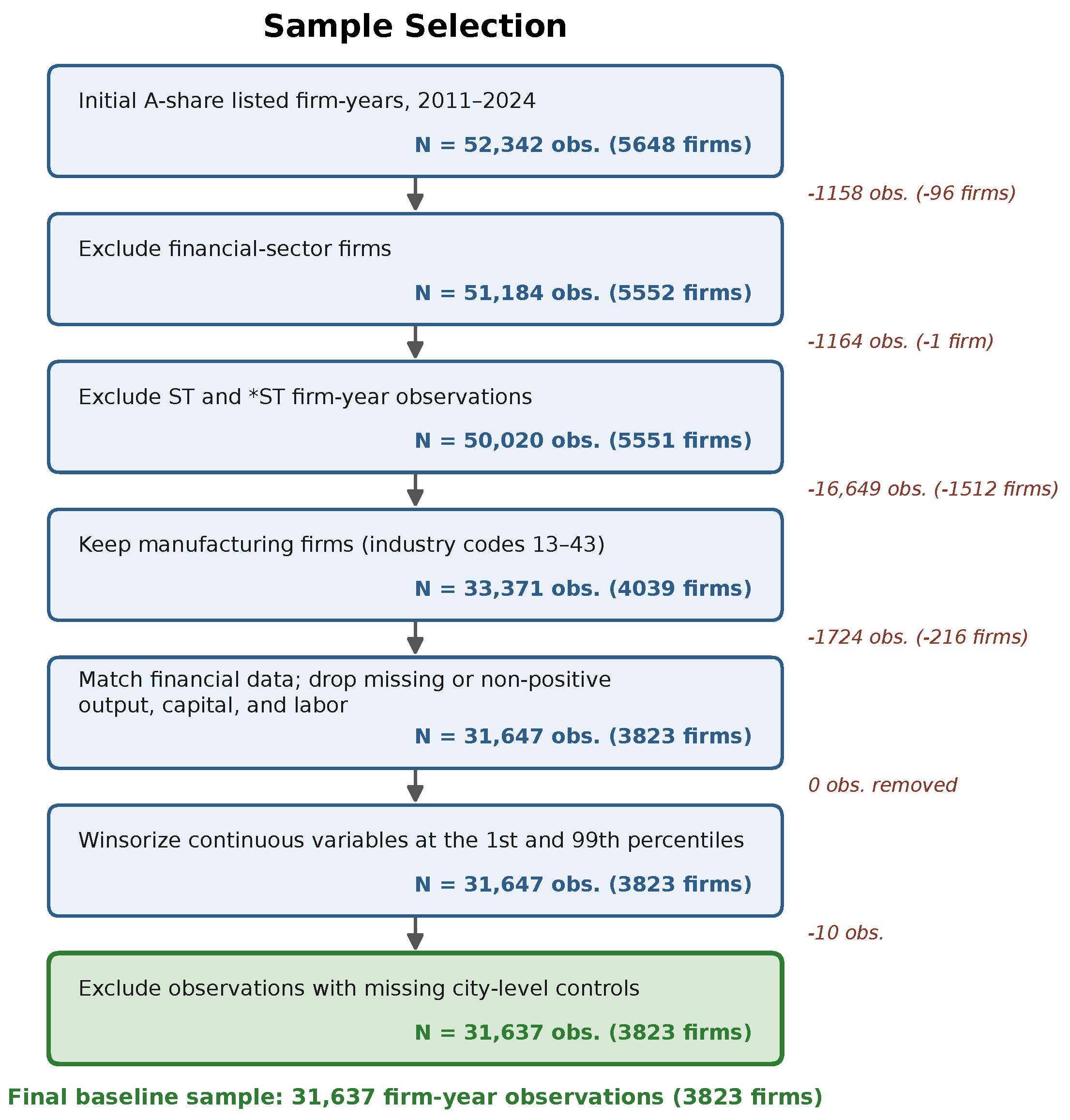
The estimation sample is constructed from A-share listed manufacturing firms (industry codes 13–43) over 2011–2024. Firm-level financial and patent data are drawn from the CSMAR and Wind databases, city-level controls from the China City Statistical Yearbook, and city-level government data platform launch timing from the China Local Government Data Openness Report. Firm–year observations with missing or non-positive output, capital, or labour values are excluded, and regressions further require non-missing control variables. Figure 1 summarizes the sample-construction process, and Table 2 reports the observations and firms remaining after each step. The panel is unbalanced by design: firms enter when they are listed or first have valid data and exit when they are delisted, suspended, or cease to have valid data. Firms that leave the sample before 2024 are retained for all years in which they have valid observations, and no post-exit observations are imputed. After the exclusions summarized in Table 2, the full sample consists of 3823 firms and 31,637 firm–year observations, with an average of approximately 8.3 observations per firm; 452 firms have their last observation before 2024. Firm fixed effects therefore exploit within-firm variation over the years in which each firm is actually observed.

Table 2. Sample construction.

Step	Excluded Obs.	Remaining Obs.	Firms
Initial A-share listed firm–year observations from CSMAR company-information and financial-statement data (2011–2024)	–	52,342	5648
Exclude financial firms	1158	51,184	5552
Exclude ST and *ST firm–year observations	1164	50,020	5551
Retain manufacturing firms (industry codes 13–43)	16,649	33,371	4039
Match with financial-statement records; exclude missing or non-positive output, capital, or labour	1724	31,647	3823
Winsorize output, capital, and labour at the 1st and 99th percentiles	0	31,647	3823
Exclude observations missing city-level controls in the merged panel	10	31,637	3823

Note: The initial sample combines CSMAR company-information and financial-statement data. Observations in the company-information panel without matching financial-statement records are excluded in the financial-statement matching step. Winsorization replaces extreme values and does not reduce the number of observations. The exclusion of ST (special treatment) and *ST (special treatment with a delisting risk warning) firms removes firm-year observations in which the firm carries ST or *ST status in that year rather than dropping entire firms; a firm is removed from the sample only if it carries ST or *ST status in every year in which it appears, which is why this step reduces the number of observations by 1164 yet the number of firms is reduced by only one. The 31,637th row is the full merged panel used for descriptive statistics; baseline regressions impose additional requirements (see Table 3).

Table 2. Sample construction.

Step	Excluded Obs.	Remaining Obs.	Firms
Initial A-share listed firm–year observations from CSMAR company-information and financial-statement data (2011–2024)	–	52,342	5648
Exclude financial firms	1158	51,184	5552
Exclude ST and *ST firm–year observations	1164	50,020	5551
Retain manufacturing firms (industry codes 13–43)	16,649	33,371	4039
Match with financial-statement records; exclude missing or non-positive output, capital, or labour	1724	31,647	3823
Winsorize output, capital, and labour at the 1st and 99th percentiles	0	31,647	3823
Exclude observations missing city-level controls in the merged panel	10	31,637	3823

Note: The initial sample combines CSMAR company-information and financial-statement data. Observations in the company-information panel without matching financial-statement records are excluded in the financial-statement matching step. Winsorization replaces extreme values and does not reduce the number of observations. The exclusion of ST (special treatment) and *ST (special treatment with a delisting risk warning) firms removes firm-year observations in which the firm carries ST or *ST status in that year rather than dropping entire firms; a firm is removed from the sample only if it carries ST or *ST status in every year in which it appears, which is why this step reduces the number of observations by 1164 yet the number of firms is reduced by only one. The 31,637th row is the full merged panel used for descriptive statistics; baseline regressions impose additional requirements (see Table 3).

Table 3. Baseline regression results.

	(1)	(2)	(3)
	DID Only	Firm + Year	Firm + Industry × Year
DID	−0.084 **	−0.103 ***	−0.082 **
	(−1.98)	(−2.67)	(−2.00)
score		−0.039	0.293
		(−0.09)	(0.73)
size		0.470 ***	0.473 ***
		(10.42)	(10.70)
soe		−0.309 ***	−0.318 ***
		(−3.92)	(−4.21)
roa		10.683 ***	10.637 ***
		(22.72)	(21.89)
growth		0.494 ***	0.519 ***
		(11.97)	(12.14)
cfo1		5.233 ***	5.151 ***
		(20.24)	(19.53)
top1		−0.744 **	−0.457 *
		(−2.58)	(−1.66)
fin_dev		0.107 ***	0.071 **
		(3.02)	(2.10)
Constant	0.723 ***	−9.143 ***	−9.297 ***
	(33.60)	(−9.22)	(−9.41)
Firm FE	Yes	Yes	Yes
Year FE	Yes	Yes	No
Industry × Year FE	No	No	Yes
N	28,682	28,682	28,677
Clusters (city)	249	249	249
$R^2$	0.566	0.630	0.648

Note: Parentheses report t-statistics. Standard errors are clustered at the city level (249 city clusters). The full merged panel contains 31,637 firm–year observations; the baseline specifications require non-missing control variables and within-firm variation (N = 28,682; 3479 firms). Column (3) drops five singleton observations under industry–year fixed effects (N = 28,677). ***, **, * denote significance at the 1%, 5%, and 10% levels.

Table 3. Baseline regression results.

	(1)	(2)	(3)
	DID Only	Firm + Year	Firm + Industry × Year
DID	−0.084 **	−0.103 ***	−0.082 **
	(−1.98)	(−2.67)	(−2.00)
score		−0.039	0.293
		(−0.09)	(0.73)
size		0.470 ***	0.473 ***
		(10.42)	(10.70)
soe		−0.309 ***	−0.318 ***
		(−3.92)	(−4.21)
roa		10.683 ***	10.637 ***
		(22.72)	(21.89)
growth		0.494 ***	0.519 ***
		(11.97)	(12.14)
cfo1		5.233 ***	5.151 ***
		(20.24)	(19.53)
top1		−0.744 **	−0.457 *
		(−2.58)	(−1.66)
fin_dev		0.107 ***	0.071 **
		(3.02)	(2.10)
Constant	0.723 ***	−9.143 ***	−9.297 ***
	(33.60)	(−9.22)	(−9.41)
Firm FE	Yes	Yes	Yes
Year FE	Yes	Yes	No
Industry × Year FE	No	No	Yes
N	28,682	28,682	28,677
Clusters (city)	249	249	249
$R^2$	0.566	0.630	0.648

Note: Parentheses report t-statistics. Standard errors are clustered at the city level (249 city clusters). The full merged panel contains 31,637 firm–year observations; the baseline specifications require non-missing control variables and within-firm variation (N = 28,682; 3479 firms). Column (3) drops five singleton observations under industry–year fixed effects (N = 28,677). ***, **, * denote significance at the 1%, 5%, and 10% levels.

Regarding data sources and city assignment, firm-level financial statements and patent data are drawn from CSMAR and Wind, analyst coverage from CSMAR, city-level economic indicators from the China City Statistical Yearbook, and platform launch timing from the China Local Government Data Openness Report. Firms are assigned to cities according to their registered address in each year. A city is defined as having launched a government data platform in the first year in which the DID indicator equals one. Municipalities directly under the central government are treated as city-level units, and province-level aggregates are used where city-level statistics are unavailable.

Table 4. Descriptive statistics.

Variable	N	Mean	SD	Min	Max
Misalloc (level)	31,637	2.036	2.146	0.104	8.398
DID	31,637	0.506	0.500	0.000	1.000
govtrasp	28,394	61.313	17.973	0.000	92.150
digpat	31,562	1.178	1.340	0.000	8.631
subsidyratio1	30,677	0.011	0.015	0.000	0.087
rd_asset_ratio	30,450	2.573	1.848	0.053	10.558
inno	31,637	2.422	1.509	0.000	6.466
lnsubsidy	30,679	15.570	3.148	0.000	22.559
score	31,637	0.360	0.205	0.069	0.991
size	31,637	22.029	1.159	19.952	25.633
soe	31,602	0.239	0.427	0.000	1.000
roa	31,637	0.040	0.061	−0.203	0.207
growth	29,241	0.137	0.325	−0.473	1.821
cfo1	31,637	0.050	0.066	−0.137	0.243
top1	31,600	0.332	0.141	0.087	0.719
fin_dev	31,326	3.938	1.563	1.334	7.511

Note: Variable definitions, units, and data sources are reported in Table 1. The sample is the full merged panel described in Section 5.1; regression samples require non-missing controls and within-firm variation.

reports the descriptive statistics for the main variables. The mean value of the firm-level misallocation measure (Misalloc) is 2.036, with a standard deviation of 2.146, a minimum of 0.104, and a maximum of 8.398. The dependent variable enters the regressions in its winsorized level form without logarithmic transformation (Section 4.2.1). The considerable dispersion in this indicator suggests that resource misallocation varies substantially across manufacturing firms: some firms are close to their optimal scale (Misalloc close to 0), while others deviate significantly. This pattern is consistent with the empirical findings of Hsieh and Klenow [4]. The core explanatory variable DID has a mean of 0.506, indicating that approximately 50.6% of firm–year observations are within the treatment period after the launch of government data platforms.

GovTrasp (index, 0–100) has a mean of 61.313 and a standard deviation of 17.973, suggesting that the overall level of government transparency across sampled cities is moderate but varies widely. The mean of digital invention patents (digpat) is 1.178, with a minimum of 0.00 and a maximum of 8.631, indicating that some firms have not yet filed digital patents, while leading firms in digital innovation have accumulated a substantial number.

Among the control variables, the mean of firm size (size) is 22.029, the proportion of state-owned enterprises (soe) is 0.239, return on assets (roa) averages 0.04, operating revenue growth rate (growth) averages 0.137, and the mean of the city-level digital economy development index (score) is 0.360.

Table 5. Correlation matrix of main variables.

	Misalloc	DID	GovTrasp	Digpat	Inno	Subratio	Rdratio	Score	Size	Soe	Roa	Growth	cfo1	top1	fin_dev
Misalloc	1.000	−0.017	0.003	−0.046	−0.038	−0.059	−0.089	−0.010	0.171	−0.104	0.442	0.193	0.320	0.032	−0.038
DID	−0.017	1.000	0.448	0.208	0.182	0.002	0.222	0.351	0.070	−0.063	−0.022	−0.035	0.029	−0.056	0.435
GovTrasp	0.003	0.448	1.000	0.154	0.140	0.016	0.161	0.421	0.042	−0.061	0.022	−0.006	0.021	−0.027	0.467
digpat	−0.046	0.208	0.154	1.000	0.727	0.113	0.399	0.101	0.428	0.124	0.006	0.033	0.012	−0.032	0.192
inno	−0.038	0.182	0.140	0.727	1.000	0.037	0.329	0.072	0.570	0.168	0.017	0.043	0.026	−0.023	0.143
subsidyratio1	−0.059	0.002	0.016	0.113	0.037	1.000	0.154	0.025	−0.156	−0.067	−0.036	−0.047	−0.087	−0.054	0.075
rd_asset_ratio	−0.089	0.222	0.161	0.399	0.329	0.154	1.000	0.142	−0.044	−0.084	0.045	0.049	0.032	−0.057	0.193
score	−0.010	0.351	0.421	0.101	0.072	0.025	0.142	1.000	−0.026	−0.105	0.024	0.011	−0.004	0.017	0.519
size	0.171	0.070	0.042	0.428	0.570	−0.156	−0.044	−0.026	1.000	0.313	0.006	0.047	0.087	0.068	0.073
soe	−0.104	−0.063	−0.061	0.124	0.168	−0.067	−0.084	−0.105	0.313	1.000	−0.101	−0.066	−0.036	0.127	0.004
roa	0.442	−0.022	0.022	0.006	0.017	−0.036	0.045	0.024	0.006	−0.101	1.000	0.273	0.476	0.164	−0.038
growth	0.193	−0.035	−0.006	0.033	0.043	−0.047	0.049	0.011	0.047	−0.066	0.273	1.000	0.026	0.008	−0.036
cfo1	0.320	0.029	0.021	0.012	0.026	−0.087	0.032	−0.004	0.087	−0.036	0.476	0.026	1.000	0.102	−0.014
top1	0.032	−0.056	−0.027	−0.032	−0.023	−0.054	−0.057	0.017	0.068	0.127	0.164	0.008	0.102	1.000	−0.001
fin_dev	−0.038	0.435	0.467	0.192	0.143	0.075	0.193	0.519	0.073	0.004	−0.038	−0.036	−0.014	−0.001	1.000

Note: Pairwise Pearson correlations on the full merged panel; the number of observations varies by pair because some variables contain missing values. Variable definitions are reported in Table 1.

reports the correlation matrix of the main variables. The correlation between the misallocation measure (Misalloc) and the treatment indicator (DID) is small and negative (−0.017), and the correlations among the remaining covariates are generally modest, suggesting that multicollinearity is unlikely to drive the baseline results.

5.2. Baseline Regression

Table 3 reports the baseline regression results with firm fixed effects and year fixed effects. Column (1) includes only the DID indicator, Column (2) adds the full set of control variables, and Column (3) replaces year fixed effects with industry–year fixed effects to further control for time-varying shocks common to firms in the same industry. All specifications are estimated on the same 28,682 firm–year observations (3479 firms) with non-missing controls and within-firm variation; Column (3) additionally drops five singleton observations under industry–year fixed effects (N = 28,677). Standard errors are clustered at the city level (249 city clusters). The DID coefficient is −0.084 in Column (1), significant at the 5% level (t = −1.98), and strengthens to −0.103, significant at the 1% level (t = −2.67), after the full set of control variables is added in Column (2). The coefficient remains negative and statistically significant at the 5% level when year fixed effects are replaced by industry–year fixed effects (−0.082, t = −2.00). City–year fixed effects are not suitable in this design because the DID indicator is defined at the city–year level and would be fully absorbed by such fixed effects. The launch of government data platforms therefore significantly reduces firm-level resource misallocation, and this result is robust to industry-specific time trends.

The magnitude of the coefficient indicates that the launch of government data platforms reduces the resource misallocation measure by 0.103 units. Relative to the sample mean of 2.036 reported in Table 4, this corresponds to a reduction of approximately 5.1% in the level of misallocation (0.103/2.036 ≈ 0.051). This result supports H1: open government data significantly improves manufacturing firms’ resource allocation efficiency.

Several control variables exhibit notable effects (interpreted with reference to Column (2), where they are included). Roa positively correlates with Misalloc (a larger value indicates greater deviation from optimal scale). Size is positively associated with Misalloc. Soe has a negative coefficient, suggesting that state-owned enterprises exhibit lower measured misallocation; because preferential access to factors is itself a potential source of distortion in this literature, we interpret this coefficient descriptively rather than as evidence of efficiency. Growth positively correlates with Misalloc, while top1 (ownership concentration) has a negative coefficient; higher concentration may mitigate or exacerbate agency problems, so we also interpret this descriptively. With firm fixed effects, the soe coefficient is identified only from firms that change ownership status.

5.3. Robustness Checks

5.3.1. Sensitivity to the Elasticity of Substitution

To assess whether the baseline result depends on the calibration of the elasticity of substitution, we reconstruct the misallocation measure under alternative values of $\sigma$ and re-estimate the baseline specification.

Table 6. Sensitivity analysis: elasticity of substitution.

	(1)	(2)	(3)	(4)
	$\mathit{\sigma }=2$	$\mathit{\sigma }=\mathbf{3}$	$\mathit{\sigma }=\mathbf{4}$	$\mathit{\sigma }=\mathbf{5}$
DID	−0.014 **	−0.103 ***	−0.800 ***	−5.214 ***
	(−2.56)	(−2.67)	(−2.71)	(−2.70)
Controls	Yes	Yes	Yes	Yes
Firm FE	Yes	Yes	Yes	Yes
Year FE	Yes	Yes	Yes	Yes
N	28,682	28,682	28,682	28,682
Clusters (city)	249	249	249	249

Note: Parentheses report t-statistics. Standard errors are clustered at the city level (249 city clusters). ***, ** denote significance at the 1% and 5% levels.

reports the DID coefficient, its t-statistic, and the sample size for $\sigma =2$, 3, 4, and 5. The estimated effect remains negative and statistically significant at the 5% level across all four values, with the coefficient increasing in magnitude with $\sigma$ as expected from the construction of the misallocation measure. These results indicate that the main finding is not driven by the specific choice of $\sigma$.

5.3.2. Sensitivity to the Required Rate of Return

The baseline specification sets the annual capital return at $R=0.10$, following Hsieh and Klenow. To assess sensitivity to this calibration, we reconstruct the misallocation measure for $R\in \{0.05,0.08,0.10,0.12,0.15,0.20\}$ and re-estimate the baseline specification.

Table 7. Sensitivity analysis: required rate of return.

	(1)	(2)	(3)	(4)	(5)	(6)
	R = 0.05	R = 0.08	R = 0.10	R = 0.12	R = 0.15	R = 0.20
DID	−0.053 ***	−0.085 ***	−0.103 ***	−0.126 ***	−0.162 ***	−0.227 ***
	(−2.71)	(−2.87)	(−2.85)	(−2.86)	(−2.88)	(−2.88)
Controls	Yes	Yes	Yes	Yes	Yes	Yes
Firm FE	Yes	Yes	Yes	Yes	Yes	Yes
Year FE	Yes	Yes	Yes	Yes	Yes	Yes
N	28,682	28,682	28,682	28,682	28,682	28,682
Clusters (city)	249	249	249	249	249	249

Note: The misallocation measure is reconstructed under each value of R with $\sigma =3$ and enters in the winsorized level form used in the baseline specification; the row $R=0.15$ can be interpreted as a 10% required return plus a 5% depreciation allowance. Parentheses report t-statistics. Standard errors are clustered at the city level (249 city clusters). *** denotes significance at the 1% level.

reports the results. The DID coefficient remains negative and statistically significant at the 1% level across the entire grid, ranging from −0.053 at $R=0.05$ to –0.227 at $R=0.20$; the row $R=0.15$ can be interpreted as a 10% required return plus a 5% depreciation allowance. These results indicate that the main finding is not driven by the calibration of R.

5.3.3. Sensitivity to the Capital Elasticity and Constant Returns to Scale

The output elasticities in Equation (3) are estimated by industry–year ordinary least squares (OLS) and are subject to the standard simultaneity problem. As an alternative, we estimate the elasticities with a control-function approach: within each industry–year cell with at least ten observations, we regress $\ln Y$ on $\ln K$, $\ln L$, and a quadratic in the log of intermediate inputs, where intermediate inputs equal operating cost plus selling, administrative, and financial expenses minus employee compensation and depreciation; the capital elasticity is then ${\alpha }_{st}={\beta }_{K,st}/({\beta }_{K,st}+{\beta }_{L,st})$. Cells without valid estimates use the economy-wide mean of the valid cells, and the resulting capital elasticity averages about 0.21.

Table 8. Sensitivity analysis: capital elasticity.

	(1)	(2)	(3)	(4)	(5)	(6)
	Regression	$\mathit{\alpha }=\mathbf{0.2}$	$\mathit{\alpha }=\mathbf{0.3}$	$\mathit{\alpha }=\mathbf{0.4}$	$\mathit{\alpha }=\mathbf{0.5}$	Control Function
DID	−0.103 ***	−0.127 ***	−0.092 ***	−0.052 ***	−0.021 **	−0.115 ***
	(−2.67)	(−2.80)	(−2.91)	(−2.80)	(−2.52)	(−2.55)
Controls	Yes	Yes	Yes	Yes	Yes	Yes
Firm FE	Yes	Yes	Yes	Yes	Yes	Yes
Year FE	Yes	Yes	Yes	Yes	Yes	Yes
N	28,682	28,682	28,682	28,682	28,682	28,682
Clusters (city)	249	249	249	249	249	249

Note: The misallocation measure is reconstructed with σ = 3 and R = 0.10 under each capital elasticity. The regression column uses the baseline industry–year OLS elasticities (mean capital elasticity about 0.13); the control-function column uses industry–year OLS with a quadratic control function in intermediate inputs (mean capital elasticity about 0.21), with cells lacking valid estimates replaced by the economy-wide mean of valid cells. Parentheses report t-statistics. Standard errors are clustered at the city level (249 city clusters). ***, ** denote significance at the 1% and 5% levels.

shows that the DID coefficient remains negative and statistically significant across constant capital elasticities of 0.2–0.5 and under the control-function estimate (−0.115, $t=-2.55$). We therefore interpret the baseline effect as robust to the simultaneity concern in the OLS estimation of output elasticities.

To assess the constant-returns-to-scale restriction imposed by Equation (4), we re-estimate the industry–year output elasticity regressions without imposing the restriction. Across 398 industry–year cells with at least five observations, the mean and median of ${\beta }_K+{\beta }_L$ are 0.981 and 0.977, respectively, and the restriction cannot be rejected at the 5% level in 82.2% of cells. We therefore follow the standard Hsieh–Klenow normalization while noting that the restriction is an approximation.

5.3.4. Heterogeneity-Robust Staggered DID Estimators

A key concern with the two-way fixed effects estimator under staggered adoption is that the coefficient may be a variance-weighted average of many two-by-two comparisons, some of which use already-treated units as controls for later-treated units, and the associated weights may be negative when treatment effects are heterogeneous across cohorts or over time. To assess the robustness of the baseline estimate, we re-estimate the average treatment effect on the treated (ATT) using the Callaway–Sant’Anna estimator [53], the Borusyak–Jaravel–Spiess imputation estimator [54], the de Chaisemartin–D’Haultfoeuille estimator [55], and the Sun–Abraham interaction-weighted estimator. Standard errors are clustered at the city level throughout. The control group is defined separately for each estimator (

Table 9. Heterogeneity-robust staggered DID estimates.

	(1)	(2)	(3)	(4)	(5)
	TWFE	CS	BJS	DCDH	SA
ATT	−0.103 ***	−0.232 **	−0.146 ***	−0.119 **	−0.158 ***
	(−2.67)	(−2.46)	(−3.09)	(−2.44)	(−3.67)
Controls	Yes	Yes	Yes	Yes	Yes
Firm FE	Yes	Yes	Yes	Yes	Yes
Year FE	Yes	Yes	Yes	Yes	Yes
Clustering	City	City	City	City	City
Control group		Never-treated	Never-treated or not-yet-treated	Switchers	Never-treated
N	28,682	22,504	18,523	14,253	27,462
Clusters (city)	249	237	237	237	237

Note: Parentheses report t-statistics. Standard errors are clustered at the city level, and each column reports its own number of city clusters. Columns (1)–(5) report the TWFE, Callaway–Sant’Anna, Borusyak–Jaravel–Spiess, de Chaisemartin–D’Haultfoeuille, and Sun–Abraham estimates. The control group differs by estimator: the Callaway–Sant’Anna and Sun–Abraham estimates use never-treated firms as controls; the Borusyak–Jaravel–Spiess estimate imputes the counterfactual from never-treated and not-yet-treated observations; and the de Chaisemartin–D’Haultfoeuille estimate is identified from units that switch treatment status. The number of observations and city clusters differ across columns because each estimator is defined on a different identifying sample: Column (1) uses the full estimation sample (28,682 firm–years with non-missing controls and within-firm variation, 249 city clusters); Column (2) includes treated units and never-treated controls with valid pre-treatment base periods and post-treatment observations; Column (3) includes treated observations whose counterfactual outcome can be imputed from untreated (never-treated or not-yet-treated) observations, dropping observations for which imputation is not feasible; Column (4) is identified from units that switch treatment status, so its observation count reflects the switcher-based design rather than the firm–year sample and is not directly comparable to the other columns; Column (5) includes treated and never-treated units with valid event-time indicators within the estimation window. The differences in N and cluster counts therefore reflect differences in identifying variation and estimands across estimators, not inconsistent sample selection. ***, ** denote significance at the 1% and 5% levels.

): the Callaway–Sant’Anna and Sun–Abraham estimators use never-treated firms as controls, the Borusyak–Jaravel–Spiess imputation estimator also uses not-yet-treated observations, and the de Chaisemartin–D’Haultfoeuille estimator is identified from units that switch treatment status.

To characterize the composition of the TWFE estimate, we first report the Goodman–Bacon decomposition [56]. Because the decomposition requires a strongly balanced panel, we construct a balanced subsample of firms observed in every year from 2011 to 2024 (721 firms, 10,094 firm–year observations) and impose the monotone treatment definition under which a firm remains treated after its city launches the platform.

Table 10. Goodman–Bacon decomposition of the TWFE estimate.

Comparison	Weight (%)	Avg. 2 × 2 DD	Contribution (%)
Timing groups	37.9	−0.128	24.3
Always treated (later vs. already-treated)	23.5	−0.238	28.2
Never treated (treated vs. never-treated)	38.6	−0.245	47.5
Total	100.0	−0.199	100.0

Note: The decomposition follows Goodman-Bacon (2021) [56] on a balanced subsample of 721 firms observed in every year from 2011 to 2024; the weighted average of the two-by-two estimates equals the TWFE coefficient on this subsample. These are descriptive decomposition weights and no standard errors are reported.

reports the decomposition. The weighted average of the two-by-two estimates equals the TWFE coefficient on this subsample (−0.199). The timing-group comparisons account for 37.9% of the weight, the always-treated comparisons for 23.5%, and the never-treated comparisons for 38.6%. In terms of the contribution to the TWFE estimate, the corresponding shares are 24.3%, 28.2%, and 47.5%. All three comparison types produce negative average two-by-two estimates, so the negative TWFE coefficient is not an artifact of already-treated units serving as controls. The balanced subsample is used only to satisfy the balanced-panel requirement of the decomposition; the full-sample baseline and heterogeneity-robust estimates are reported below.

In the full sample, 96 of 272 cities (35.3%) have no treated firm–year observations by 2024. Because listed manufacturing firms are concentrated in early-adopting cities, these never-treated cities account for only 3384 of 31,637 firm–year observations (10.7%) and 376 of 3823 firms (9.8%). We therefore do not rely on the TWFE estimate alone and corroborate the baseline result with the heterogeneity-robust estimators below. The full sample spans 272 cities; the baseline estimation sample contains 249 city clusters because the remaining cities have no within-firm variation in the data-platform indicator or no city-level controls. Each regression table reports the cluster count corresponding to its own estimation sample, so the cluster counts stated in the table headers and the table notes are consistent.

Table 9 reports the results. The Callaway–Sant’Anna estimate is −0.232 (SE = 0.094, p = 0.014), the Borusyak–Jaravel–Spiess estimate is −0.146 (SE = 0.047, p = 0.002), the de Chaisemartin–D’Haultfoeuille estimate is −0.119 (SE = 0.049, p = 0.015), and the Sun–Abraham estimate is −0.158 (SE = 0.043, p < 0.001). All estimates are negative and statistically significant at conventional levels, corroborating the TWFE baseline and indicating that the negative effect is not an artifact of heterogeneous treatment timing under staggered adoption.

5.3.5. Parallel Trend Test

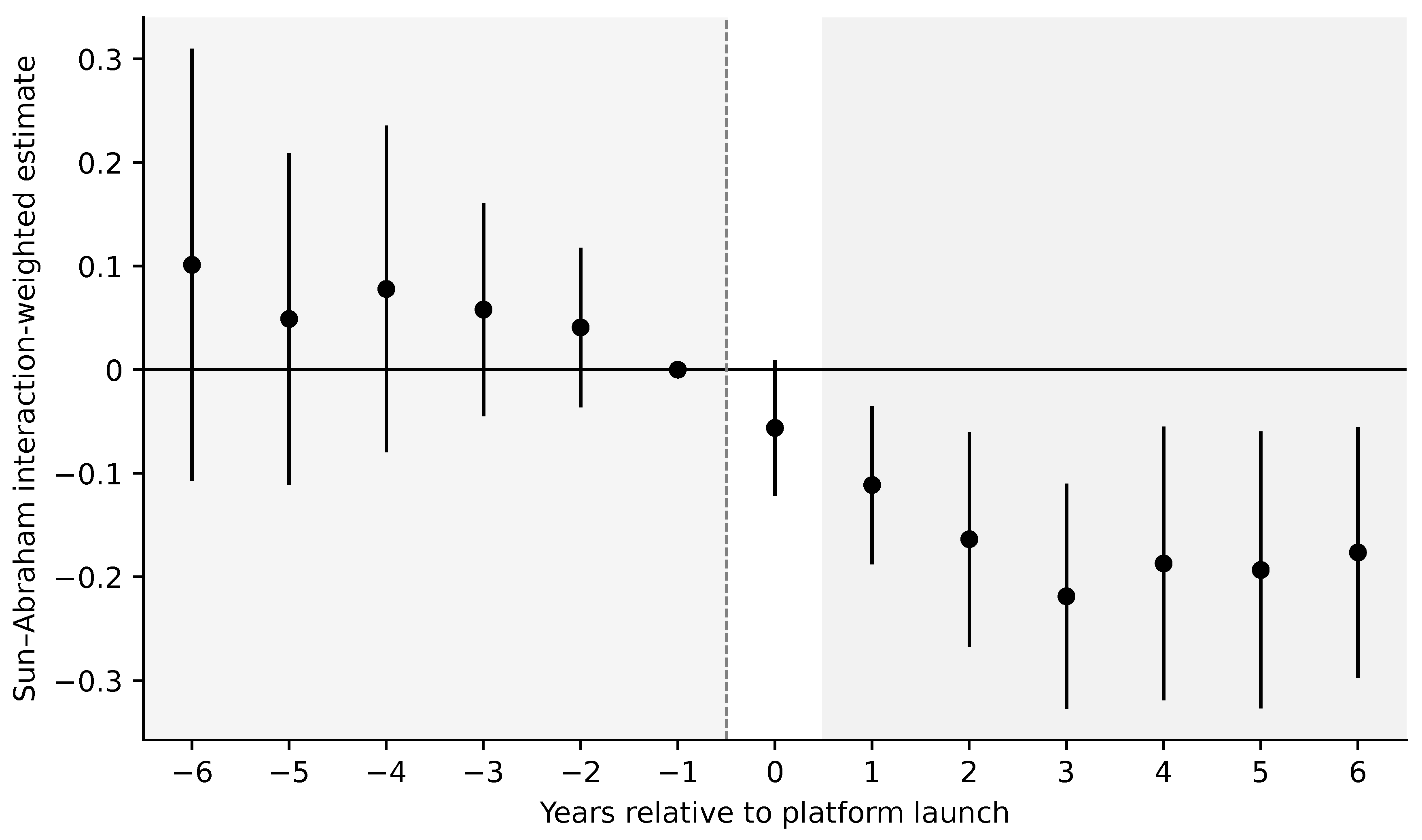
A key identifying assumption of the staggered DID design is that firms in treated and untreated cities exhibit parallel trends in resource allocation efficiency before the launch of the government data platform. To avoid the interpretation problems of a conventional two-way fixed-effects event study under staggered adoption, we follow the interaction-weighted estimator of Sun and Abraham [57]. This estimator weights cohort-specific dynamic effects by their cohort shares, so the resulting estimates are not contaminated by already-treated units serving as controls.

Figure 2 presents the Sun–Abraham interaction-weighted estimates. All pre-treatment coefficients from periods −6 to −2 are individually insignificant, and a joint Wald test of the five pre-treatment coefficients fails to reject the null that they are jointly zero (F(5, 236) = 0.484, p = 0.788), providing no evidence against the parallel-trends assumption. After the platform launch, the estimates become negative and are statistically significant in periods 1–6, with coefficients ranging from −0.111 to −0.219. The average post-treatment effect over periods 0–6 is −0.158 (SE = 0.043, $p<0.001$), corroborating the baseline result.

Regarding the timing of platform adoption, the staggered rollout followed a policy-driven, top-down path rather than reflecting purely local self-selection. As described in Section 2.1, China’s open government data policy progressed from centrally initiated pilot projects to nationwide promotion, and local launches were concentrated in specific waves (

Table 11. Distribution of cities by platform launch cohort.

Launch Year	Cities	Share (%)	Cumulative (%)	Firm–Year Obs.
2012	3	1.1	1.1	3731
2014	1	0.4	1.5	822
2015	5	1.8	3.3	1371
2016	3	1.1	4.4	3282
2017	4	1.5	5.9	981
2018	29	10.7	16.5	6217
2019	32	11.8	28.3	3555
2020	31	11.4	39.7	4255
2021	33	12.1	51.8	2039
2022	10	3.7	55.5	703
2023	17	6.2	61.8	799
2024	8	2.9	64.7	498
Never treated	96	35.3	100.0	3384
Total	272	100.0		31,637

Note: A city is assigned to the cohort in which its government data platform first launches. Firm–year observations count all observations of firms located in cities of the given cohort over the full sample period.

), with eastern and central cities adopting earlier than western and northeastern ones. This institutionalized rollout, driven by national policy targets and administrative directives, weakens the concern that adoption timing was chosen on the basis of local economic conditions. Nevertheless, to the extent that early-adopting cities differ in observable respects, we address this directly: the Sun–Abraham event study and the joint Wald test of the pre-treatment coefficients (F(5, 236) = 0.484, p = 0.788) show no significant differential trends before platform launch, propensity score matching balances observable firm and city characteristics, and the heterogeneity-robust estimators restrict comparisons to never-treated controls. While no design can fully rule out selection on unobservables correlated with adoption timing, the combination of the policy-driven rollout pattern and the absence of pre-existing trend differences supports the interpretation that the estimated effect reflects the policy itself rather than divergent prior trajectories of early adopting cities.

5.3.6. Placebo Test

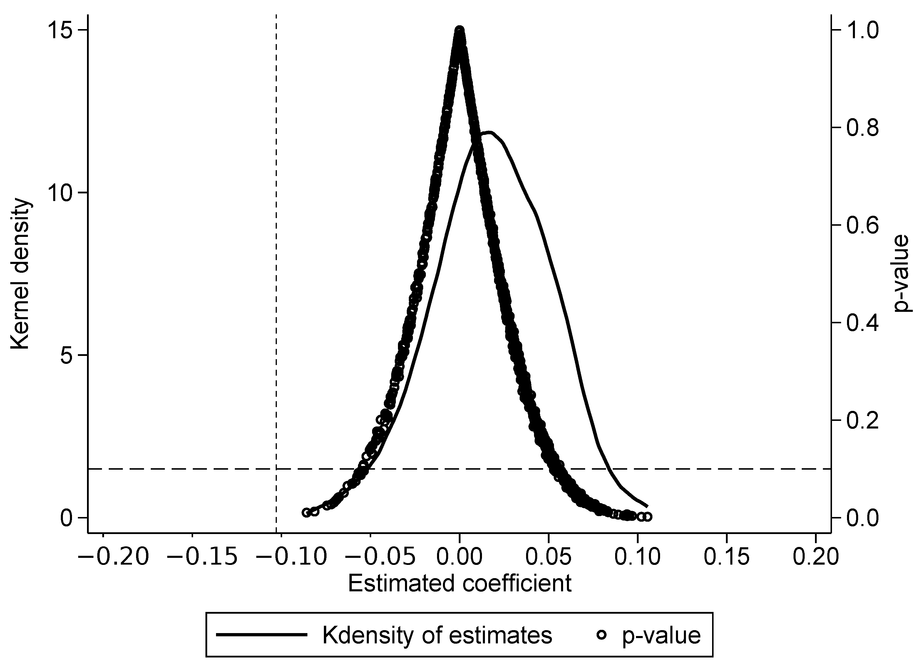
To further verify that the baseline results are not driven by unobserved confounding factors, we conduct a placebo test by randomly assigning the treatment status across cities while maintaining the same proportion of treated observations as in the actual sample. This randomization procedure is repeated 1000 times, generating a distribution of placebo DID coefficients (Figure 3).

The mean of the placebo coefficients is centred around zero and follows a normal distribution, while the actual estimated coefficient from Table 3 (−0.103) falls well outside the 95% confidence interval of the placebo distribution. This result confirms that the baseline finding is unlikely to be driven by chance or by unobserved city-specific shocks.

5.3.7. Propensity Score Matching

To address potential selection bias arising from the non-random placement of government data platforms, we employ propensity score matching (PSM). We first estimate a logit model of the DID indicator on the full set of control variables (score, size, soe, roa, growth, cfo1, top1, fin_dev); the pseudo $R^2$ is 0.187. Because treatment is staggered across years, we match within each calendar year: each treated firm–year is matched to the nearest untreated firm–year in the same year with a calliper of 0.05 on the propensity score (1:1 nearest-neighbour matching with replacement and common support ) (

Table 12. Robustness check: PSM-DID estimation.

	PSM-DID
DID	−0.122 **
	(−2.00)
score	0.155
	(0.34)
size	0.479 ***
	(10.37)
soe	−0.283 ***
	(−3.83)
roa	10.374 ***
	(22.54)
growth	0.517 ***
	(12.61)
cfo1	5.210 ***
	(19.48)
top1	−0.888 ***
	(−3.14)
fin_dev	0.111 ***
	(3.01)
Firm FE	Yes
Year FE	Yes
N	16,920
Clusters (city)	241
$R^2$	0.806

Note: Matching is performed within each calendar year (1:1 nearest neighbour, calliper 0.05, replacement, common support). Parentheses report t-statistics. Standard errors are clustered at the city level (241 city clusters). ***, ** denote significance at the 1% and 5% levels.

).

Table 13. PSM covariate balance.

Variable	Before	After
score	0.752	0.458
size	0.141	−0.108
soe	−0.126	−0.037
roa	−0.042	0.035
growth	−0.071	0.021
cfo1	0.067	−0.016
top1	−0.105	0.024
fin_dev	0.970	0.350

Note: Standardized differences are computed as the difference in means between treated and control observations divided by the pooled standard deviation, before and after within-year matching.

reports standardized differences before and after matching. Matching substantially reduces imbalance for firm-level covariates, although the city-level covariates score and fin_dev remain somewhat imbalanced after matching (standardized differences of 0.46 and 0.35); we therefore interpret the PSM estimate as supplementary evidence.

The DID estimation on the matched sample yields a coefficient of −0.122 (t = −2.00, p = 0.047), consistent with the baseline estimate. The sample falls from 28,682 to 16,920 observations because observations without a suitable same-year match are discarded.

5.3.8. Alternative Explained Variable

To verify that the baseline results are not driven by the choice of dependent variable, we replace it with an alternative measure of investment efficiency. Following McNichols and Stubben [58], we estimate the expected level of investment from a regression of a firm’s current investment on its determinants, including lagged Tobin’s Q, operating cash flow, asset growth, and lagged investment, with industry and year fixed effects. The residual from this regression measures the deviation of actual investment from the model-implied expected investment. We use the signed residual as the alternative dependent variable. The sample is not restricted to overinvesting firms, and we do not take the absolute value of the residual, so the specification does not condition on the outcome. The rationale is that when firms face severe allocative distortions, their investment decisions systematically deviate from the efficient level, manifesting as overinvestment or underinvestment.

Table 14. Robustness: alternative DV (investment expectation residual).

	Investment Residual
DID	−0.002 **
	(−2.03)
score	0.010 *
	(1.66)
size	0.001
	(1.35)
soe	−0.002
	(−0.95)
roa	0.065 ***
	(7.26)
growth	0.021 ***
	(10.36)
cfo1	−0.052 ***
	(−7.02)
top1	0.018 ***
	(3.01)
fin_dev	0.000
	(0.12)
Firm FE	Yes
Year FE	Yes
N	24,568
Clusters (city)	248
$R^2$	0.192

Note: Parentheses report t-statistics. Standard errors are clustered at the city level (248 city clusters). The dependent variable is the signed residual from the McNichols–Stubben investment expectation model; the sample is not restricted to overinvesting firms and the absolute residual is not used. ***, **, * denote significance at the 1%, 5%, and 10% levels.

reports the results. The DID coefficient is −0.002 and is statistically significant at the 5% level once standard errors are clustered at the treatment (city) level (t = −2.03, p = 0.043). The negative coefficient implies that the signed investment residual declines after the platform launch, consistent with the corrective effect on over-allocated firms documented in the directional analysis.

5.3.9. Excluding Alternative Explanations

To rule out the possibility that the baseline results are driven by concurrent policies rather than by open government data per se, we control for several policy shocks that occurred during the sample period. Specifically, we include indicators for the following: the Big Data Comprehensive Pilot Zone policy, the Broadband China strategy, and the National Smart City pilot. Each of these policies may affect firms’ information environment and resource allocation through different channels. Columns (4) and (5) further control for firm-level innovation capacity (inno2) and digital transformation (dig), respectively, to ensure that the estimated effect of open government data is not confounded by firm-level heterogeneity in innovation and digital capabilities. The construction of inno2 and dig follows Li et al. [51] and Qi et al. [52], as detailed in the control variables subsection.

The DID coefficient remains statistically significant at least at the 10% level after controlling for each of these policy indicators, and at the 5% level when firm-level innovation capacity or digital transformation is added, with magnitudes ranging from −0.103 to −0.079. This suggests that the baseline effect is not confounded by these concurrent policy initiatives or by firm-level innovation and digitalization. Columns (1)–(3) use 25,047 observations because the city-level policy indicators are missing for part of the sample, while Columns (4) and (5) use 28,682 and 28,595 observations (

Table 15. Robustness: excluding concurrent policies.

	(1)	(2)	(3)	(4)	(5)
DID	−0.082 *	−0.079 *	−0.084 *	−0.103 **	−0.100 **
	(−1.74)	(−1.81)	(−1.80)	(−2.54)	(−2.46)
smart	0.130
	(1.57)
broadband		0.001
		(0.03)
bigdata			0.116
			(1.59)
inno2				−0.059 ***
				(−3.81)
dig					−0.086
					(−0.90)
Controls	Yes	Yes	Yes	Yes	Yes
Firm FE	Yes	Yes	Yes	Yes	Yes
Year FE	Yes	Yes	Yes	Yes	Yes
N	25,047	25,047	25,047	28,682	28,595
Clusters (city)	243	243	243	249	249
$R^2$	0.633	0.633	0.633	0.628	0.627

Note: Parentheses report t-statistics. Standard errors are clustered at the city level (cluster counts per column). ***, **, * denote significance at the 1%, 5%, and 10% levels.

).

5.3.10. Double Machine Learning

To further address potential functional form misspecification and high-dimensional controls, we employ the double/debiased machine learning (DML) approach of Chernozhukov et al. [59]. The DML estimator uses a partialling-out procedure with Lasso-based regularization to flexibly control for a large set of covariates while avoiding regularization bias.

The DML estimates range from −0.102 to −0.104 across control sets and learners and remain statistically significant at the 1% level with standard errors clustered at the treatment (city) level (t between −2.62 and −2.81). The consistency between the DML estimates and the baseline OLS estimate provides evidence that the estimated effect of open government data on resource allocation efficiency is robust to nonlinearities and high-dimensional confounding (

Table 16. Double Machine Learning (DML) results.

Variable	(1)	(2)	(3)	(4)	(5)	(6)
DID	−0.102 ***	−0.103 ***	−0.104 ***	−0.102 ***	−0.102 ***	−0.103 ***
	(0.038)	(0.038)	(0.037)	(0.039)	(0.038)	(0.038)
Control set (1st-order)	Yes	Yes	Yes	Yes	Yes	Yes
Control set (2nd-order)	No	Yes	Yes	No	Yes	Yes
Control set (3rd-order)	No	No	Yes	No	No	Yes
Learner	OLS	OLS	OLS	Lasso	Lasso	Lasso
Fixed effects	Yes	Yes	Yes	Yes	Yes	Yes
Clusters (city)	249	249	249	249	249	249
Observations	28,682	28,682	28,682	28,682	28,682	28,682

Note: Parentheses report standard errors clustered at the city level (249 city clusters). The estimation sample uses 28,682 firm–year observations with complete controls and within-firm variation. Columns (1)–(3) use OLS learners and Columns (4)–(6) use Lasso learners; control sets are first-, first-plus-second-, and first-plus-second-plus-third-order terms, respectively. In the low-dimensional control sets used here, Lasso approximates OLS, so the estimates are similar across columns. *** denotes significance at the 1% level.

).

5.4. Pre-Treatment Comparability and Adoption-Timing Robustness

Platform adoption is not randomly assigned across cities. The launch cohorts in Table 11 show that eastern and central cities, which are on average larger and more developed, adopted earlier.

Table 17. Pre-treatment city characteristics by adoption timing.

	Early	Late	Never	Early − Never	Late − Never	F-Stat
econ_dev	10.786	10.830	10.732	0.054 **	0.098 ***	7.27 ***
				(2.20)	(3.86)
score	0.250	0.190	0.169	0.082 ***	0.022 ***	140.81 ***
				(14.37)	(5.07)
fin_dev	2.727	2.426	2.931	−0.205 ***	−0.505 ***	27.65 ***
				(−3.23)	(−7.44)
openness	0.291	0.118	0.096	0.195 ***	0.022 ***	145.67 ***
				(13.52)	(3.00)
pop_density	6.086	5.659	5.607	0.479 ***	0.052	49.03 ***
				(8.90)	(1.00)
edu_exp	0.183	0.171	0.171	0.012 ***	−0.000	22.77 ***
				(6.01)	(−0.04)
gov_interv	0.187	0.187	0.227	−0.040 ***	−0.040 ***	34.62 ***
				(−6.86)	(−7.27)
fisc_press	0.097	0.112	0.152	−0.055 ***	−0.040 ***	54.06 ***
				(−9.40)	(−7.30)
Cities	108	68	96

Note: Each characteristic is measured at the city level before the platform launch (for treated cities) or over the sample period (for never-treated cities). Early and late adopters are split at the median city launch year (2020). The columns “Early − Never” and “Late − Never” report the mean difference relative to never-adopting cities, with t-statistics from two-sample Welch tests in parentheses. F-statistics and their significance test the joint equality of the three group means. *** and ** denote significance at the 1% and 5% levels.

compares pre-treatment city characteristics across early-, late-, and never-adopting cities, where early and late adopters are split at the median city launch year (2020) and each city’s characteristics are measured before its platform launch. Early adopters are on average more economically developed (econ_dev, openness), more digitally advanced (score), and more densely populated, while exhibiting lower financial development (fin_dev), lower government intervention (gov_interv), and lower fiscal pressure (fisc_press). The differences relative to never-adopting cities are statistically significant for most characteristics, confirming that adoption timing is systematically correlated with economic development, digital infrastructure, and administrative capacity.

To assess whether these systematic differences bias the estimate, we re-estimate the baseline specification with two additional controls for adoption-timing endogeneity (

Table 18. Robustness to the endogeneity of adoption timing.

	(1) Baseline	(2) Region × Year FE	(3) Reg. × Year FE + Pre-Treat.
DID	−0.103 ***	−0.100 ***	−0.111 ***
	(−2.67)	(−2.67)	(−3.12)
Controls	Yes	Yes	Yes
Firm FE	Yes	Yes	Yes
Year FE	Yes	Yes	Yes
Region × Year FE	No	Yes	Yes
Pre-treat. char. × trend	No	No	Yes
N	28,682	28,682	28,258
Clusters (city)	249	249	234

Note: Parentheses report t-statistics. Standard errors are clustered at the city level. The dependent variable is the winsorized level measure of resource misallocation. Column (1) reproduces the baseline result for reference. Column (2) adds region×year fixed effects, where the region is East, Central, or West. Column (3) additionally adds pre-treatment city characteristics (economic development, digital economy index, government intervention, and financial development) interacted with a linear time trend; its sample is slightly smaller because a small number of observations lack these city characteristics. *** denotes significance at the 1% level.

). Column (2) adds region × year fixed effects (East/Central/West interacted with year), so that identification comes only from within-region variation in adoption timing and any region-specific shocks are absorbed. Column (3) additionally adds pre-treatment city development characteristics (initial economic development, digital economy index, government intervention, and financial development) interacted with a linear time trend, allowing cities that differ in these initial characteristics to trend differently. In both specifications, the DID coefficient remains negative and statistically significant (−0.100 and −0.111, respectively), similar in magnitude to the baseline estimate. This indicates that the estimated effect is not driven by the endogenous timing of platform adoption.

5.5. Heterogeneity Analysis

To evaluate whether the baseline effect differs across groups, we report subsample estimates and, for each split, a full-sample interaction regression that formally tests the difference between groups. Grouping variables are fixed at pre-treatment values using the same rule as the directional classification in Section 6.2: for treated firms and cities, the value in the year immediately before platform launch; for never-treated units and units without an observation in that year, the value in the first sample year; and, only if that value is missing, the unit-level full-sample mean. In each interaction regression, the main effect of the time-invariant group dummy is absorbed by firm fixed effects, so the difference between groups is identified by the coefficient on the DID × Group interaction.

5.5.1. Enterprise Internal Characteristics (Micro Dimension)

We first examine heterogeneity by firm ownership type. The sample is split into state-owned enterprises (SOEs) and non-SOEs. The DID coefficient is −0.158 (significant at the 5% level) for SOEs and −0.072 (not statistically significant) for non-SOEs. However, the full-sample interaction DID × SOE is −0.065 (t = −1.16, p = 0.249), indicating that the difference between SOEs and non-SOEs is not statistically significant. We therefore do not claim a differential effect by ownership. The ownership split follows the firm’s current ownership status; ownership changes are rare in the sample.

We further examine heterogeneity by firms’ subsidy dependency, measured by the subsidy-to-revenue ratio (subsidyratio1) fixed at its pre-treatment value. The DID coefficients are −0.125 (t = −2.13) for high-dependency firms and −0.071 (t = −1.24) for low-dependency firms, and the full-sample interaction DID × high subsidy is 0.025 (t = 0.39, p = 0.698). The difference between the two groups is therefore not statistically significant, and we do not claim differential effects by subsidy dependence.

Heterogeneity by labour quality is examined by classifying firms according to the median of the pre-treatment share of skilled employees (technical, financial, and sales staff). The high-skill coefficient is −0.047 (not statistically significant), and the low-skill coefficient is −0.139 (significant at the 1% level). However, the full-sample interaction DID × high skill is 0.006 (t = 0.10, p = 0.921), so the difference between the two groups is not statistically significant, and we do not claim differential effects by labour quality (

Table 19. Heterogeneity: enterprise characteristics.

	Ownership		Subsidy Dep.		Labor Quality
Variable	(1) SOE	(2) Non-SOE	(3) High	(4) Low	(5) High	(6) Low
DID	−0.158 **	−0.072	−0.125 **	−0.071	−0.047	−0.139 ***
	(−2.21)	(−1.64)	(−2.13)	(−1.24)	(−0.73)	(−2.75)
Controls	Yes	Yes	Yes	Yes	Yes	Yes
Firm FE	Yes	Yes	Yes	Yes	Yes	Yes
Year FE	Yes	Yes	Yes	Yes	Yes	Yes
N	7211	21,426	14,233	14,449	13,979	14,703
Clusters (city)	173	226	197	216	180	227
$R^2$	0.593	0.642	0.600	0.646	0.630	0.632

Note: Subsidy dependence and labour quality are fixed at pre-treatment values (year before platform launch, first sample year, or unit-level full-sample mean); ownership follows the firm’s current status. Parentheses report t-statistics. Standard errors are clustered at the city level (cluster counts per column). ***, ** denote significance at the 1% and 5% levels.

).

5.5.2. Industry Technical Characteristics (Meso Dimension)

We examine heterogeneity by industry digital intensity. Industries are classified into high and low digital-intensity groups based on a fixed set of two-digit manufacturing industries (17, 18, and 26–33) that rely intensively on digital technologies. These industries account for roughly 38% of the estimation sample; after dropping firms with no within-group variation, the subsamples contain 10,937 and 17,695 observations. The DID coefficient is −0.187 (significant at the 5% level) for high-digital-intensity industries and −0.002 for low-digital-intensity industries. The full-sample interaction DID × high digital intensity is −0.157 (t = −2.27, p = 0.024), confirming that the efficiency-improving effect is significantly stronger in high-digital-intensity industries.

We also examine heterogeneity by analyst coverage, using the pre-treatment value of analyst attention. The high-coverage coefficient is −0.096 (not statistically significant) and the low-coverage coefficient is −0.103 (significant at the 5% level). However, the full-sample interaction DID × high coverage is −0.105 (t = −1.63, p = 0.104), so the difference between the two groups is not statistically significant, and we do not claim differential effects by analyst coverage (

Table 20. Heterogeneity: industry characteristics.

	Digital Intensity		Analyst Coverage
Variable	(1) High	(2) Low	(3) High	(4) Low
DID	−0.187 **	−0.002	−0.096	−0.103 **
	(−2.59)	(−0.06)	(−1.58)	(−2.01)
Controls	Yes	Yes	Yes	Yes
Firm FE	Yes	Yes	Yes	Yes
Year FE	Yes	Yes	Yes	Yes
N	10,937	17,695	14,674	14,008
Clusters (city)	214	203	196	210
$R^2$	0.639	0.629	0.643	0.598

Note: Analyst coverage is fixed at its pre-treatment value; industry digital intensity is a time-invariant industry classification. Parentheses report t-statistics. Standard errors are clustered at the city level (cluster counts per column). ** denotes significance at the 5% level.

).

5.5.3. External Macro Environment (Macro Dimension)

We first examine heterogeneity by city size, using the pre-treatment city population. In the full-sample interaction specification, the DID coefficient for small cities is −0.181 (significant at the 1% level), the total effect for large cities is 0.001 (not statistically significant), and the interaction DID × large is 0.182 (t = 3.10, p = 0.002). The formal test therefore confirms that the efficiency-improving effect of open government data is concentrated in smaller cities, where alternative information channels are less developed and the marginal value of open data is larger (

Table 21. Heterogeneity: macro environment.

	City Size		Digital Economy Level
Variable	(1) Large	(2) Small	(3) High	(4) Low
DID	−0.047	−0.124 **	−0.056	−0.131 **
	(−0.85)	(−2.10)	(−1.31)	(−2.23)
Controls	Yes	Yes	Yes	Yes
Firm FE	Yes	Yes	Yes	Yes
Year FE	Yes	Yes	Yes	Yes
N	14,163	14,512	15,223	13,449
Clusters (city)	30	219	43	206
$R^2$	0.602	0.649	0.636	0.624

Note: City size and regional digital economy development are fixed at pre-treatment values. Parentheses report t-statistics. Standard errors are clustered at the city level (cluster counts per column). ** denotes significance at the 5% level.

).

We further examine heterogeneity by regional digital economy development level, using the pre-treatment city digital economy index. In the full-sample interaction specification, the DID coefficient for low-digital-development cities is −0.223 (significant at the 1% level), the total effect for high-digital-development cities is 0.019 (not statistically significant), and the interaction DID × high is 0.242 (t = 3.79, p < 0.001). This confirms that open government data plays a meaningful role in narrowing the regional “digital divide” by providing a particularly strong efficiency-improving effect in regions where digital development is less advanced, consistent with the catch-up effect hypothesis. Because the large-city and high-digital-development subsamples contain only 30 and 43 city clusters, respectively, these subsample estimates should be interpreted with caution; the formal tests above use the full sample (249 city clusters) (

Table 22. Heterogeneity: formal tests of group differences.

Split	(1) DID	(2) DID × Group	(3) Group = 1 Total	(4) p (DID × Group)	(5) N	(6) Clusters
Ownership (SOE)	−0.084 **	−0.065	−0.149 **	0.249	28,682	249
	(−1.99)	(−1.16)	(−2.51)
Subsidy dependence (high)	−0.114 **	0.025	−0.089 *	0.698	28,682	249
	(−2.08)	(0.39)	(−1.84)
Labour quality (high)	−0.105 **	0.006	−0.099 **	0.921	28,682	249
	(−1.98)	(0.10)	(−2.00)
Industry digital intensity (high)	−0.042	−0.157 **	−0.200 ***	0.024	28,682	249
	(−0.95)	(−2.27)	(−3.23)
Analyst coverage (high)	−0.046	−0.105	−0.152 ***	0.104	28,682	249
	(−0.95)	(−1.63)	(−2.76)
City size (large)	−0.181 ***	0.182 ***	0.001	0.002	28,682	249
	(−3.28)	(3.10)	(0.03)
Digital economy development (high)	−0.223 ***	0.242 ***	0.019	<0.001	28,682	249
	(−3.83)	(3.79)	(0.42)
Firm FE	Yes	Yes	Yes
Year FE	Yes	Yes	Yes

Note: Each row reports a full-sample regression of y on DID, the group dummy, DID × Group, and the control variables with firm and year fixed effects. The Group main effect is absorbed by firm fixed effects. Parentheses report t-statistics. Standard errors are clustered at the city level (249 city clusters). Grouping variables are fixed at pre-treatment values, except ownership, which follows the firm’s current status. ***, **, * denote significance at the 1%, 5%, and 10% levels.

).

6. Further Analysis

6.1. Mechanism Analysis

This section tests three potential channels through which open government data may affect firms’ resource allocation efficiency: governance transparency, digital innovation, and fiscal resource allocation. It is important to note that because the structural characteristics of the observable data vary across these mechanisms, we employ identification strategies tailored to each channel rather than applying a uniform mediation regression framework. Each mechanism’s analytical logic and regression approach are described below.

6.1.1. Test of the Government Governance Transparency Channel

Governance transparency is hypothesized to affect resource allocation efficiency through two pathways. First, it reduces information asymmetry between governments and market participants, enabling firms to make more accurate investment and operational decisions. Second, it strengthens external oversight of public resource allocation, improving the efficiency of fiscal spending. To examine this channel, we estimate the reduced-form effect of the data platform on the city-level government transparency index (GovTrasp) and, following the suggestion to treat transparency as a moderator rather than a mediator, test whether the policy effect on resource allocation efficiency varies with the level of government transparency.

Table 23. Transparency channel tests.

	(1)	(2)	(3)
Variable	GovTrasp	Misalloc	Misalloc
DID	2.861	−0.177	−0.394 ***
	(1.35)	(−1.53)	(−3.09)
govtrasp		−0.001
		(−0.57)
DID × govtrasp		0.001
		(0.90)
govtrasp_pre			0.005
			(0.72)
DID × govtrasp_pre			0.006 **
			(2.57)
score	29.597 *	−0.022	−0.064
	(2.11)	(−0.06)	(−0.14)
size	0.186	0.322 ***	0.291 ***
	(0.71)	(8.10)	(7.34)
soe	0.426	−0.141 **	−0.150 ***
	(0.72)	(−2.46)	(−2.85)
roa	2.031	5.752 ***	5.886 ***
	(1.00)	(16.30)	(15.21)
growth	0.433 *	0.350 ***	0.343 ***
	(1.98)	(8.69)	(7.46)
cfo1	−1.561	3.383 ***	3.364 ***
	(−1.23)	(12.84)	(12.86)
top1	−1.957	−0.775 ***	−0.574 **
	(−1.06)	(−3.47)	(−2.50)
fin_dev	−1.734	0.015	0.040
	(−1.64)	(0.60)	(1.31)
Firm fixed effects	Yes	Yes	Yes
Year fixed effects	Yes	Yes	Yes
Observations (N)	26,046	26,046	25,123
Clusters (city)	246	246	238
$R^2$	0.734	0.644	0.631

Note: Column (1) reports the reduced-form effect of the data platform on the city-level government transparency index (GovTrasp). Column (2) adds the contemporaneous interaction DID × GovTrasp to the efficiency equation; Column (3) interacts DID with the pre-treatment baseline GovTrasp_pre (the city average before platform launch; the full-sample average is used for never-treated cities). Parentheses report t-statistics. Standard errors are clustered at the city level (cluster counts per column). GovTrasp is winsorized at the 1st and 99th percentiles in all three columns. Column (3) uses a smaller sample because cities without any pre-launch GovTrasp observations are excluded. ***, **, * denote significance at the 1%, 5%, and 10% levels.

reports the results. Column (1) uses GovTrasp as the dependent variable: the DID coefficient is 2.861 but is not statistically significant once standard errors are clustered at the treatment (city) level (t = 1.35, p = 0.180). Column (2) adds the contemporaneous interaction between DID and GovTrasp to the efficiency equation: the DID coefficient is −0.177 (t = −1.53), the interaction coefficient is 0.001 and statistically insignificant (t = 0.90), and the coefficient on GovTrasp itself is also insignificant (t = −0.57). The contemporaneous interaction is therefore not statistically significant.

Column (3) instead interacts DID with the pre-treatment baseline level of government transparency (GovTrasp_pre, the city average before platform launch; the full-sample average is used for never-treated cities). The interaction coefficient is 0.006, significant at the 5% level (t = 2.57, p = 0.011), indicating that the efficiency-improving effect of open government data is significantly stronger in cities with lower initial transparency; evaluated at the sample mean of the baseline index (49.6), the total DID effect is −0.103. Although the contemporaneous interaction is insignificant, the pre-treatment moderation test provides direct evidence that the transparency environment shapes the allocative effect of open data, consistent with the interpretation that open data delivers larger marginal benefits where pre-existing information channels are weaker, mirroring the heterogeneity results for regional digital development.

6.1.2. Test of the Digital Innovation Empowerment Channel

Digital technology is a potential micro-level transmission pathway through which open government data may affect firms’ resource allocation efficiency. Following the approach of the innovation channel, we use the number of digital invention patent applications (digpat) as a firm-level measure of digital innovation capability. This indicator is defined as ln(digital invention patent applications + 1), with digital categories identified by screening patent titles and IPC codes. Compared with text-mining-based digital transformation indices, digital invention patent data are subject to substantive examination and thus carry higher technical credibility.

To examine this channel, we estimate the reduced-form effect of open government data on firms’ digital innovation output without including the mechanism variable in the outcome equation.

Table 24. Digital innovation channel test.

Variable	Digital Patents (Digpat)
DID	0.024
	(0.82)
score	0.084
	(0.47)
size	0.474 ***
	(17.31)
soe	−0.041
	(−0.73)
roa	−0.131
	(−0.99)
growth	−0.061 ***
	(−3.28)
cfo1	0.024
	(0.26)
top1	0.231
	(1.39)
fin_dev	0.040 **
	(2.11)
Firm fixed effects	Yes
Year fixed effects	Yes
Observations (N)	28,662
Clusters (city)	249
$R^2$	0.781

Note: The dependent variable is the firm-level digital innovation measure digpat (ln of one plus digital invention patent applications), winsorized at the 1st and 99th percentiles. The regression reports the reduced-form effect of the data platform on digpat without including the mechanism variable in the outcome equation. Parentheses report t-statistics. Standard errors are clustered at the city level (249 city clusters). ***, ** denote significance at the 1% and 5% levels.

reports the results: the DID coefficient is 0.024 but is not statistically significant once standard errors are clustered at the treatment (city) level (t = 0.82, p = 0.415). Although the point estimate is positive and consistent in sign with H3, the digital innovation channel is not supported by the data under treatment-level inference, and we report the channel as unsupported rather than claiming partial mediation.

6.1.3. Test of the Subsidy Resource Allocation Optimization Channel

The allocation of fiscal subsidies across firms is a key institutional factor influencing resource allocation efficiency. We examine whether the policy shifts subsidy allocation toward more innovative or higher-R&D-intensity firms, using two reduced-form interaction specifications.

The first specification uses the logarithm of subsidies received (lnsubsidy) as the dependent variable and interacts the DID indicator with lagged firm innovation (L.inno). Column (1) of

Table 25. Subsidy allocation channel tests.

Variable	(1) Lnsubsidy	(2) SubsidyRatio
DID	0.225	0.001
	(1.58)	(1.32)
L.inno	0.044
	(1.38)
DID × L.inno	−0.037
	(−0.91)
L.rd_asset_ratio		0.000
		(0.15)
DID × L.rd_asset_ratio		−0.0001
		(−0.47)
Controls	Yes	Yes
Firm fixed effects	Yes	Yes
Year fixed effects	Yes	Yes
Observations (N)	26,037	25,070
Clusters (city)	247	245
$R^2$	0.307	0.533

Note: Column (1) reports the interaction of the DID indicator with lagged firm innovation (L.inno) in a regression of ln(subsidy); Column (2) reports the interaction with lagged R&D intensity (L.rd_asset_ratio) in a regression of subsidy intensity (subsidies over operating revenue). Parentheses report t-statistics. Standard errors are clustered at the city level (cluster counts per column).

reports the results: the coefficient on DID × L.inno is −0.037 and statistically insignificant (t = −0.91). The second specification uses subsidy intensity (subsidyratio1) as the dependent variable and interacts DID with lagged R&D intensity (L.rd_asset_ratio). Column (2) reports the results: the coefficient on DID × L.rd_asset_ratio is −0.0001 and statistically insignificant (t = −0.47). Neither specification indicates that the policy significantly redirects subsidy allocation toward more innovative or higher-R&D-intensity firms, and the subsidy allocation channel is therefore not supported by the data.

6.2. Direction Identification of Resource Allocation Efficiency

The baseline regression results indicate that open government data significantly improves resource allocation efficiency among manufacturing firms. However, these findings do not yet answer a more nuanced question: which type of resource allocation distortion does open government data primarily address? Specifically, does open government data improve allocative efficiency by curbing excessive investment by capital-overallocated firms—a “corrective effect”—or by alleviating financing constraints faced by capital-underallocated firms—a “relief effect”? The answer to this question is crucial for understanding the micro-level mechanisms through which open government data improves resource allocation efficiency.

Following the analytical framework of Hsieh and Klenow [4], we decompose the direction of resource misallocation along two dimensions based on the distortion measures derived from the model: the capital distortion direction and the output expansion direction. Both classifications are directly constructed from the distortion measures defined in Section 4.2.1, providing two complementary identification approaches.

First, the capital distortion direction. Recall from Equation (7) the definition of capital distortion:

$$1+{\tau }_{K,ist}={\displaystyle \frac{{\alpha }_{st}{Y}_{ist}}{K_{ist}}}·{\displaystyle \frac{1-{\tau }_{Y,ist}}{R}}$$

(10)

This indicator captures the deviation of the effective capital cost borne by the firm from the market equilibrium level. When $1+{\tau }_{K,ist}<1$, the firm faces an effective capital cost below the market average, implying that capital is overallocated to the firm (overK = 1). When $1+{\tau }_{K,ist}>1$, the firm faces an effective capital cost above the market average, implying that capital is underallocated (underK = 1, with overK = 0).

Second, the output expansion direction. Recall from Equation (8) the ratio of the optimal output to actual output:

$${\displaystyle \frac{Y_{ist}^{opt}}{Y_{ist}}}={(1-{\tau }_{Y,ist})}^{-(\sigma -1)}{(1+{\tau }_{K,ist})}^{-{\alpha }_{st}(\sigma -1)}$$

(11)

Define $Y_{\mathrm{opt}\_\mathrm{ratio}}\equiv Y_{ist}^{opt}/Y_{ist}$. When $Y_{\mathrm{opt}\_\mathrm{ratio}}>1$, the firm’s actual output is below its optimal level, suggesting the firm should expand its scale (expand = 1). When $Y_{\mathrm{opt}\_\mathrm{ratio}}<1$, the firm’s actual output exceeds its optimal level, suggesting the firm should contract its scale (contract = 1, with expand = 0). Note that the dependent variable in the baseline regression, $\mathrm{Misalloc}=|Y_{\mathrm{opt}\_\mathrm{ratio}}-1|$, is derived from the absolute value of this ratio; the directional classification here splits the sign.

It is important to note that these two classification perspectives are complementary but distinct. The overK/underK classification directly identifies the direction of capital factor misallocation, whereas the expand/contract classification reflects the deviation direction of total output (including both capital and labour). The former is a factor-input identification, while the latter is an output-level identification; together they constitute the complete directional identification framework from factor inputs to output.

Because the directional dummies are mechanically constructed from the same optimal-to-actual output ratio that defines the dependent variable, we fix each firm’s classification at its pre-treatment value and hold it constant throughout the sample period. Specifically, for firms whose city launched a government data platform, the classification is taken from the year immediately before platform launch; for never-treated firms, and for treated firms without an observation in the year before launch, the classification is taken from the firm’s first sample year (and, if that value is also missing, the unit-level full-sample mean). This removes the contemporaneous conditioning on the outcome and preserves the direction as a pre-determined firm characteristic. Of the 3164 treated firms in the estimation sample, 1555 (49.1%) lack an observation in the year immediately before launch and are therefore classified using their first sample year, which may postdate platform launch; as a robustness check, we re-estimate the specification excluding these firms, which yields qualitatively identical results (see the note to

Table 26. Directional identification regression results.

Variable	(1) Capital Distortion Direction	(2) Output Expansion Direction
DID (open government data)	0.000	$-0.126$ ***
	(0.00)	(−3.19)
overK (capital overallocation)	(absorbed)
DID × overK (interaction)	$-0.127$ ***
	(−3.40)
expand		(absorbed)
DID × expand		$0.512$ ***
		(9.24)
Linear combinations
DID (overK = 0/expand = 0)	0.000	$-0.126$ ***
	(0.00)	(−3.19)
DID + DID × overK (overK = 1)	$-0.127$ ***
	(−3.15)
DID + DID × expand (expand = 1)		$0.386$ ***
		(7.07)
Controls	Yes	Yes
Firm fixed effects	Yes	Yes
Year fixed effects	Yes	Yes
Observations	28,682	28,682
Clusters (city)	249	249
$R^2$	0.631	0.628

Note: Classification dummies are fixed at the year before platform launch, or the firm’s first sample year (and, if that value is missing, the unit-level full-sample mean) for never-treated firms and for treated firms without a pre-launch observation, and are held constant over the sample period; their main effects are absorbed by firm fixed effects. Of the 3164 treated firms, 1555 are classified using the first-sample-year rule. Excluding these 1555 firms yields qualitatively identical results (capital-overallocated total −0.127, $t=-3.02$; expansion-needing total 0.399, $t=6.19$). Parentheses report t-statistics. Standard errors are clustered at the city level. Linear combination rows report the total DID effect for each group and its formal test. *** denotes significance at the 1% level.

). The main effects of the resulting time-invariant dummies are absorbed by firm fixed effects, so the regressions identify the differential effect through the interaction with DID.

Table 26 presents the directional identification regression results on the full estimation sample (28,682 firm–year observations clustered in 249 cities). Column (1) uses the pre-treatment capital overallocation dummy (overK) as the grouping variable. The DID coefficient for capital-underallocated firms (overK = 0) is 0.000 and statistically insignificant ($t=0.00$); the interaction DID × overK is −0.127, significant at the 1% level ($t=-3.40$). The formally tested linear combination for capital-overallocated firms (overK = 1) is −0.127, significant at the 1% level ($t=-3.15$, $p=0.002$). This suggests that open government data primarily alleviates the efficiency loss from excessive investment by capital-overallocated firms. Column (2) uses the pre-treatment output expansion dummy (expand). For firms not classified as needing to expand (expand = 0), the DID coefficient is −0.126, significant at the 1% level ($t=-3.19$); the interaction DID × expand is 0.512, significant at the 1% level ($t=9.24$). The linear combination for expansion-needing firms (expand = 1) is 0.386 and statistically significant ($t=7.07$, $p<0.001$). The policy therefore has a significant corrective effect on capital-overallocated firms, while it significantly increases the deviation from the optimal scale for firms classified as needing to expand.

These results carry clear economic implications: open government data improves resource allocation efficiency primarily by strengthening market discipline to curb excessive investment by capital-overallocated firms—a “corrective effect.” The output-expansion direction shows a parallel asymmetry: the policy significantly reduces misallocation among firms not classified as needing to expand, while the total effect for expansion-needing firms is positive and statistically significant (0.386, $t=7.07$), indicating that the policy significantly increases the deviation from optimal scale for firms that should be expanding rather than relieving their constraints. This finding is consistent with the theoretical logic that open government data reduces information asymmetry in factor markets: by making public information more accessible, the policy enables market participants and external monitors to better evaluate firms’ investment decisions, disciplining the investment behaviour of overcapitalized firms. It is worth noting that this mechanism operates at the level of the information environment in factor markets rather than through the specific intermediation channels examined in Section 6.1, none of which exhibit a statistically significant direct effect; the directional evidence instead indicates that the efficiency gains materialize through the disciplining of overinvestment, rather than through a direct relaxation of financing constraints.

7. Conclusions

This study exploits the staggered rollout of city-level government data platforms in China as a quasi-natural experiment and draws on panel data of listed manufacturing firms from 2011 to 2024 to systematically examine the effect of open government data on firms’ resource allocation efficiency. The baseline regression results show that the launch of government data platforms significantly reduces the degree of firm-level resource misallocation, with the efficiency-improving effect concentrated among capital-overallocated firms identified by the directional analysis. This finding is robust to propensity score matching, exclusion of concurrent policy shocks, double machine learning, and an alternative investment-efficiency specification in which the dependent variable is the signed residual from the McNichols–Stubben investment expectation model (DID = −0.00190, t = −2.03, p = 0.043).

Mechanism analysis provides channel-level evidence on how open government data affects resource allocation efficiency. The governance transparency channel is not supported by the data: open government data does not exhibit a statistically significant effect on city-level government transparency once standard errors are clustered at the treatment level. A complementary moderation test indicates that the efficiency-improving effect is significantly stronger in cities with lower initial government transparency (interaction coefficient 0.006, t = 2.57); we interpret this pattern as reflecting larger marginal benefits of open data where pre-existing information channels are weaker, rather than as evidence that transparency is a transmission mechanism. The digital innovation channel is not supported: the reduced-form effect of open government data on firm-level digital invention patent applications is positive but not statistically significant under treatment-level clustering. The subsidy resource allocation channel is not supported: neither the responsiveness of subsidy allocation to firm innovation nor to R&D intensity changes significantly after the platform launch under treatment-level clustering.

Several considerations may account for the absence of statistically significant effects along these intermediate channels despite the significant baseline effect. First, the transparency index, digital patent counts, and subsidy measures capture only specific, observable aspects of the relevant mechanisms; the allocative benefits of open data may operate through broader, less readily measurable improvements in the information environment that are not fully reflected in these indicators. Second, firm-level adjustments along these channels may take longer to materialize than the sample period permits. Third, the reduced-form specifications and moderation tests we employ are designed to detect average changes, and they cannot rule out heterogeneous responses that offset one another at the mean. These considerations qualify, rather than overturn, the interpretation that the efficiency gains operate primarily through the disciplining of inefficient investment documented in the directional analysis.

Directional identification reveals a clear asymmetry in the resource allocation effect of open government data. Using directional classifications fixed at pre-treatment values, the policy primarily reduces efficiency losses among capital-overallocated firms through a “corrective effect” that curbs excessive investment, while significantly increasing the deviation from optimal scale for firms classified as needing to expand, suggesting that the mechanism operates through disciplining inefficient investment rather than relaxing financing constraints.

Heterogeneity analysis conducted across three dimensions—firm characteristics, industry characteristics, and regional environment—uses formal full-sample interaction tests to compare groups. Differences by ownership, subsidy dependence, labour quality, and analyst coverage are not statistically significant under city-level clustering. Heterogeneity is statistically significant only for industry digital intensity, city size, and regional digital economy development: the efficiency-improving effect is concentrated in high-digital-intensity industries, smaller cities, and regions with lower levels of digital economy development. Together, these patterns indicate that open government data helps bridge the regional “digital divide” rather than exacerbating it [60], and that its allocative benefits are shaped by a combination of firm capabilities, industry conditions, and the surrounding information environment.

These findings carry several policy implications. First, governments should continue to advance the construction of open government data platforms, steadily improving dimensions such as data standardization and machine readability. Open government data directly enhances resource allocation efficiency in factor markets, and the directional evidence indicates that this improvement operates primarily by disciplining the investment behaviour of over-allocated firms, providing empirical support for deepening market-oriented reform of production factors. Second, the documented asymmetry between the “corrective effect” on over-allocated firms and the significant worsening of the deviation from optimal scale among expansion-needing firms implies that open data policies are better suited to disciplining inefficient investment than to easing financing constraints. Complementary policies—such as credit market reforms and targeted financial support—remain necessary to address the distinct frictions faced by firms that should expand but remain constrained. Third, local governments should recognize that the benefits of open government data depend on complementary conditions. Coordinating data platforms with talent development programs and information intermediaries can help firms make more effective use of open data. Fourth, firms should regard open government data as a strategic opportunity for digital transformation and innovation-driven development, increasing investment in data analysis capabilities and R&D talent to fully realize the potential benefits of open government data policies.

From the perspective of sustainable development, the findings of this study carry implications that go beyond firm-level efficiency. Resource misallocation wastes scarce capital, labour, and energy inputs and raises the resource and emission intensity of production, so improving the efficiency of factor allocation is itself a sustainability objective. By providing causal evidence that institutionalized data openness curbs inefficient investment and disciplines the allocation of public and private resources, this study suggests that open government data may serve as a low-cost, scalable instrument for sustainable resource governance. These results speak to the socio-economic dimension of sustainability and complement the United Nations Sustainable Development Goals, in particular decent work and economic growth (SDG 8); industry, innovation, and infrastructure (SDG 9); and responsible consumption and production (SDG 12). More broadly, the study illustrates an integrated approach in which digital governance, market efficiency, and sustainable development reinforce one another: data openness improves the information environment of factor markets, which in turn reduces the wasteful use of resources and supports inclusive, higher-quality growth. These insights are relevant not only for China but also for other developing economies designing data-governance reforms as part of their sustainability strategies.

Several limitations should be acknowledged. The Hsieh–Klenow industry benchmarks are computed from listed manufacturing firms only, a highly selected group, so the estimated level of misallocation may not generalize to the full manufacturing population. The output elasticities in Equation (3) are estimated by industry–year OLS and are subject to the standard simultaneity problem; our control-function-based alternative yields a similar treatment effect (−0.115, $t=-2.55$). Constant returns to scale are imposed through the normalization in Equation (4), although the restriction cannot be rejected in most industry–year cells. VAT payable is estimated from cash-flow data using statutory rates. These concerns are addressed with the sensitivity analyses reported above.

Relative to closely related work on open government data and resource allocation, this study contributes by constructing a firm-level Hsieh–Klenow misallocation measure, addressing staggered-adoption bias with heterogeneity-robust estimators, and identifying the corrective rather than relief nature of the policy effect. In summary, this study provides causal evidence on the economic and social consequences of open government data from the perspective of resource allocation efficiency. As the market-oriented reform of production factors deepens, high-quality open government data has become an important institutional tool. Through well-designed institutional arrangements and enhanced coordination among open data policies, corporate strategies, and digital infrastructure, China can further improve firms’ resource allocation efficiency under resource constraints and promote higher-quality economic development.

References

1. Attard, J.; Orlandi, F.; Scerri, S.; Auer, S. A systematic review of open government data initiatives. Gov. Inf. Q. 2015, 32, 399–418. [Google Scholar] [CrossRef] [Scilit]
2. Zuiderwijk, A.; Janssen, M. Open data policies, their implementation and impact: A framework for comparison. Gov. Inf. Q. 2014, 31, 17–29. [Google Scholar] [CrossRef] [Scilit]
3. Mikalef, P.; Lemmer, K.; Schaefer, C.; Ylinen, M.; Fjørtoft, S.O.; Torvatn, H.Y.; Gupta, M.; Niehaves, B. Enabling AI capabilities in government agencies: A study of determinants for European municipalities. Gov. Inf. Q. 2022, 39, 101596. [Google Scholar] [CrossRef] [Scilit]
4. Hsieh, C.T.; Klenow, P.J. Misallocation and Manufacturing TFP in China and India. Q. J. Econ. 2009, 124, 1403–1448. [Google Scholar] [CrossRef] [Scilit]
5. Brandt, L.; Tombe, T.; Zhu, X. Factor market distortions across time, space and sectors in China. Rev. Econ. Dyn. 2013, 16, 39–58. [Google Scholar] [CrossRef] [Scilit]
6. Hopenhayn, H.A. Firms, misallocation, and aggregate productivity: A review. Annu. Rev. Econ. 2014, 6, 735–770. [Google Scholar] [CrossRef] [Scilit]
7. Xu, C.; Chen, Y.; Dai, J. Open government data and resource allocation efficiency: Evidence from China. Appl. Econ. 2024, 57, 2887–2904. [Google Scholar] [CrossRef] [Scilit]
8. Jiang, W.; Li, J. Digital transformation and its effect on resource allocation efficiency and productivity in Chinese corporations. Technol. Soc. 2024, 78, 102638. [Google Scholar] [CrossRef] [Scilit]
9. Hope, O.; Jiang, S.; Vyas, D. Government transparency and firm-level operational efficiency. J. Bus. Financ. Account. 2022, 49, 752–777. [Google Scholar] [CrossRef] [Scilit]
10. Goldfarb, A.; Tucker, C. Digital economics. J. Econ. Lit. 2019, 57, 3–43. [Google Scholar] [CrossRef] [Scilit]
11. Wang, H.; Ye, F.; Yin, J.Y. How public data opening boosts enterprise effective investment: From the perspective of capacity utilization. China Ind. Econ. 2024, 8, 137–153. (In Chinese) [Google Scholar] [CrossRef]
12. Lin, Z.; Yin, Y.; Liu, L.; Wang, D. SciSciNet: A large-scale open data lake for the science of science research. Sci. Data 2023, 10, 315. [Google Scholar] [CrossRef] [Scilit]
13. North, D.C. Institutions, Institutional Change and Economic Performance; Cambridge University Press: Cambridge, UK, 1990. [Google Scholar]
14. Park, S.; Gil-Garcia, J.R. Understanding Transparency and Accountability in Open Government Ecosystems: The Case of Health Data Visualizations in a State Government. In Proceedings of the 18th Annual International Conference on Digital Government Research, Staten Island, NY, USA, 7–9 June 2017; pp. 39–47. [Google Scholar] [CrossRef] [Scilit]
15. OECD. Enhanced Access to Publicly Funded Data for Science, Technology and Innovation; Technical Report; OECD Publishing: Paris, France, 2020. [Google Scholar] [CrossRef] [Scilit]
16. David, J.M.; Venkateswaran, V. Information, misallocation, and aggregate productivity. Q. J. Econ. 2016, 131, 943–1005. [Google Scholar] [CrossRef] [Scilit]
17. Syverson, C. What determines productivity? J. Econ. Lit. 2011, 49, 326–365. [Google Scholar] [CrossRef] [Scilit]
18. Ubaldi, B. Open Government Data: Towards Empirical Analysis of Open Government Data Initiatives; Technical Report 22, OECD Working Papers on Public Governance; OECD Publishing: Paris, France, 2013. [Google Scholar] [CrossRef]
19. Janssen, M.; Charalabidis, Y.; Zuiderwijk, A. Benefits, Adoption Barriers and Myths of Open Data and Open Government. Inf. Syst. Manag. 2012, 29, 258–268. [Google Scholar] [CrossRef] [Scilit]
20. Wu, W.Q.; Li, J.H.; Zhang, L.Y.; Zhao, Y. Public data resources and enterprise total factor productivity: A quasi-natural experiment based on local government data opening. Syst. Eng. Theory Pract. 2024, 44, 1815–1833. (In Chinese) [Google Scholar]
21. Li, X.; Liu, Z.; Ye, Y. Public data and corporate employment: Evidence from the launch of Chinese public data platform. Econ. Anal. Policy 2024, 84, 124–144. [Google Scholar] [CrossRef] [Scilit]
22. Shan, J.; Zhang, L.; Wang, J. Data elements and corporate stock dividends: A quasi-natural experiment based on government data openness. Int. Rev. Financ. Anal. 2025, 97, 103846. [Google Scholar] [CrossRef] [Scilit]
23. Xu, R.; Xu, C. How Government Open Data Platforms Affect Corporate ESG Performance. Sustainability 2025, 17, 9768. [Google Scholar] [CrossRef] [Scilit]
24. Akerlof, G.A. The Market for Lemons: Quality Uncertainty and the Market Mechanism. Q. J. Econ. 1970, 84, 488–500. [Google Scholar] [CrossRef] [Scilit]
25. Jones, C.I.; Tonetti, C. Nonrivalry and the economics of data. Am. Econ. Rev. 2020, 110, 2819–2858. [Google Scholar] [CrossRef] [Scilit]
26. Restuccia, D.; Rogerson, R. The Causes and Costs of Misallocation. J. Econ. Perspect. 2017, 31, 151–174. [Google Scholar] [CrossRef] [Scilit]
27. Stigler, G.J. The economics of information. J. Political Econ. 1961, 69, 213–225. [Google Scholar] [CrossRef] [Scilit]
28. Veldkamp, L.; Chung, C. Data and aggregate economy. J. Econ. Lit. 2024, 62, 458–484. [Google Scholar] [CrossRef] [Scilit]
29. Montes, G.C.; Albuquerque Bastos, J.C.; de Oliveira, A.J. Fiscal transparency, government effectiveness and government spending efficiency: Some international evidence based on panel data approach. Econ. Model. 2019, 79, 211–225. [Google Scholar] [CrossRef] [Scilit]
30. Chen, C.; Neshkova, M.I. The effect of fiscal transparency on corruption: A panel cross-country analysis. Public Adm. 2020, 98, 226–243. [Google Scholar] [CrossRef] [Scilit]
31. Elberry, N.A.; Naert, F.; Goeminne, S. The Impact of Fiscal Openness on Public Spending Technical Efficiency in Developing Countries. Public Perform. Manag. Rev. 2022, 45, 254–281. [Google Scholar] [CrossRef] [Scilit]
32. Dupor, B.; Karabarbounis, M.; Kudlyak, M.; Mehkari, M.S. Regional Consumption Responses and the Aggregate Fiscal Multiplier. Rev. Econ. Stud. 2023, 90, 2982–3021. [Google Scholar] [CrossRef] [Scilit]
33. Baba-Yara, F.; Boons, M.; Tamoni, A. Persistent and transitory components of firm characteristics: Implications for asset pricing. J. Financ. Econ. 2024, 154, 103808. [Google Scholar] [CrossRef] [Scilit]
34. Wu, K.; Liu, S.; Zhu, M.; Qu, Y. The impact of digital transformation on resource mismatch of Chinese listed companies. Sci. Rep. 2024, 14, 9011. [Google Scholar] [CrossRef] [Scilit]
35. Ding, J.; Yin, Y.; Kuang, J.; Ding, D.; Madsen, D.; Yang, K. The impact of enterprise digital transformation on financial mismatch: Empirical evidence from listed companies in China. Financ. Res. Lett. 2024, 66, 105677. [Google Scholar] [CrossRef] [Scilit]
36. Yang, T.; Wu, K.; Du, X.; Yuan, G. Does the digital transformation of enterprises affect capital mismatch? Evidence from Chinese listed firms. PLoS ONE 2025, 20, e0313674. [Google Scholar] [CrossRef] [Scilit]
37. Gao, X.; Feng, H. Data-Driven Business Innovation Processes: Evidence from Authorized Data Flows in China. Systems 2024, 12, 280. [Google Scholar] [CrossRef] [Scilit]
38. Jetzek, T.; Avital, M.; Bjorn-Andersen, N. Data-Driven Innovation through Open Government Data. J. Theor. Appl. Electron. Commer. Res. 2014, 9, 15–16. [Google Scholar] [CrossRef] [Scilit]
39. Wang, Q.; Hu, J. Open government data and firms’ open innovation: Evidence from listed firms in China. J. Technol. Transf. 2025, 1–26. [Google Scholar] [CrossRef] [Scilit]
40. Wang, J.; Zhou, X.; Ma, Y.; Choi, Y. Public Data Elements and Enterprise Digital Transformation: A Quasi-Natural Experiment Based on Open Government Data Platforms for Sustainable Urban Planning. Sustainability 2025, 17, 4676. [Google Scholar] [CrossRef] [Scilit]
41. Sun, S.; Zheng, T.; Pan, H.; Gu, X. Open government data and enterprise innovation: Evidence from China. Appl. Econ. 2025, 57, 1–15. [Google Scholar] [CrossRef] [Scilit]
42. Jin, X. Government Subsidies, Resource Misallocation and Manufacturing Productivity. China Financ. Econ. Rev. 2018, 7, 74–95. [Google Scholar] [CrossRef] [Scilit]
43. Weng, L.; Xu, C.; Yi, M. Resource misallocation in China: Biased subsidies versus credit discrimination. Econ. Model. 2024, 134, 106699. [Google Scholar] [CrossRef] [Scilit]
44. Kornai, J. The Soft Budget Constraint. Kyklos 1986, 39, 3–30. [Google Scholar] [CrossRef] [Scilit]
45. Gao, X. Zombie firms, state subsidies and aggregate productivity. Economica 2025, 92, 507–547. [Google Scholar] [CrossRef] [Scilit]
46. Branstetter, L.G.; Li, G.; Ren, M. Picking Winners? Government Subsidies and Firm Productivity in China; Technical Report w30699; National Bureau of Economic Research: Cambridge, MA, USA, 2022. [Google Scholar] [CrossRef] [Scilit]
47. Wei, Z.Y. The impact of digital economy development on resource allocation efficiency of manufacturing enterprises. J. Quant. Technol. Econ. 2022, 39, 66–85. (In Chinese) [Google Scholar] [CrossRef]
48. Yu, X.C. Research on the stickiness of VAT burden of Chinese manufacturing enterprises: An empirical analysis based on A-share listed companies. J. Cent. Univ. Financ. Econ. 2020, 2, 18–28. (In Chinese) [Google Scholar]
49. Zhang, T.H.; Zhang, S.H. Biased policies, resource allocation and the efficiency of state-owned enterprises. Econ. Res. J. 2016, 51, 126–139. (In Chinese) [Google Scholar]
50. Zhao, T.; Zhang, Z.; Liang, S.K. Digital economy, entrepreneurial activity and high-quality development: Empirical evidence from Chinese cities. Manag. World 2020, 36, 65–76. (In Chinese) [Google Scholar] [CrossRef]
51. Li, C.T.; Yan, X.W.; Song, M.; Yang, W. FinTech and corporate innovation: Evidence from NEEQ listed companies. China Ind. Econ. 2020, 1, 81–98. (In Chinese) [Google Scholar] [CrossRef]
52. Qi, H.J.; Cao, X.Q.; Liu, Y.X. The impact of digital economy on corporate governance: From the perspective of information asymmetry and managerial irrational behavior. Reform 2020, 4, 50–64. (In Chinese) [Google Scholar]
53. Callaway, B.; Sant’Anna, P.H.C. Difference-in-Differences with Multiple Time Periods. J. Econom. 2021, 225, 200–230. [Google Scholar] [CrossRef] [Scilit]
54. Borusyak, K.; Jaravel, X.; Spiess, J. Revisiting Event-Study Designs: Robust and Efficient Estimation. Rev. Econ. Stud. 2024, 91, 3253–3285. [Google Scholar] [CrossRef] [Scilit]
55. de Chaisemartin, C.; D’Haultfœuille, X. Two-Way Fixed Effects Estimators with Heterogeneous Treatment Effects. Am. Econ. Rev. 2020, 110, 2964–2996. [Google Scholar] [CrossRef] [Scilit]
56. Goodman-Bacon, A. Difference-in-Differences with Variation in Treatment Timing: Theory and Applications. J. Econom. 2021, 225, 254–277. [Google Scholar] [CrossRef] [Scilit]
57. Sun, L.; Abraham, S. Estimating Dynamic Treatment Effects in Event Studies with Heterogeneous Treatment Effects. J. Econom. 2021, 225, 175–199. [Google Scholar] [CrossRef] [Scilit]
58. McNichols, M.F.; Stubben, S.R. Does earnings management affect firms’ investment decisions? Account. Rev. 2008, 83, 1571–1603. [Google Scholar] [CrossRef] [Scilit]
59. Chernozhukov, V.; Chetverikov, D.; Demirer, M.; Duflo, E.; Hansen, C.; Newey, W.; Robins, J. Double/debiased machine learning for treatment and structural parameters. Econom. J. 2018, 21, C1–C68. [Google Scholar] [CrossRef] [Scilit]
60. Tan, L.; Pei, J. Open Government Data and the Urban-Rural Income Divide in China: An Exploration of Data Inequalities and Their Consequences. Sustainability 2023, 15, 9867. [Google Scholar] [CrossRef] [Scilit]
Figure 1. Sample-construction flowchart.
Sustainability 18 08796 g001
Figure 2. Sun–Abraham interaction-weighted event-study estimates. Joint test of zero pre-treatment coefficients (periods −6 to −2): F(5, 236) = 0.484, p = 0.788.
Sustainability 18 08796 g002
Figure 3. Placebo test: distribution of 1000 randomly assigned treatment effects.
Sustainability 18 08796 g003