Article

Exploring the Spatially Heterogeneous Patterns of Sustainable Environmental Development in the Yangtze River Economic Belt: A Prefecture-Level City Perspective


1
School of Geography and Oceanography, Minjiang University, Fuzhou 350108, China
2
School of Earth Science and Spatial Information Engineering, Hunan University of Science and Technology, Xiangtan 411100, China
3
School of Geosciences and Info-Physics, Central South University, Changsha 410012, China
*
Author to whom correspondence should be addressed.
Sustainability 2026, 18(17), 8765; https://doi.org/10.3390/su18178765
Submission received: 15 April 2026 / Revised: 28 July 2026 / Accepted: 6 August 2026 / Published: 27 August 2026
(This article belongs to the Special Issue Geographical Information Technology and Urban Sustainable Development)

Abstract

Understanding the spatial distribution and associated factors of sustainable environmental development (SED) is crucial for effectively formulating action plans aimed at achieving the environment-related Sustainable Development Goals (SDGs). Because of spatial heterogeneity characterized by non-uniform distributions of SED within a region, the use of a single or aggregated value at the national or provincial scale in existing research obscures internal variabilities and fails to adequately reveal the spatial disparities in the progress of environment-related SDGs. Consequently, this study aims to investigate the spatially heterogeneous patterns of SED in prefecture-level cities within the Yangtze River Economic Belt (YREB), China—a critical economic zone characterized by stark intra-regional disparities and pressing environmental challenges. To achieve this objective, the SED index is first constructed using principal component weighted aggregation to quantify the SED status, local Moran’s I is then employed to identify heterogenous patters of the spatial distribution patterns of SED, and geographical random forest is utilized to explore spatially varying association patterns between SED and influences factors. In the YREB, the findings indicate the following key insights: (1) SED has generally shown a positive trend across most cities from 2013 to 2021, with approximately 30% experiencing a downward trend, particularly in Jiangxi, Hubei, and Hunan Provinces; (2) the number of high- or low-value aggregation clusters has decreased, concurrent with an increase in spatial variability; (3) human activity disturbance and population density have been identified as significant factors influencing SED, with a notable impact in cities across Sichuan, Chongqing, Guizhou, and Hubei Provinces. This research contributes technical support and a scientific foundation for evaluating and enhancing SED.

1. Introduction

Global environmental issues, driven by intense social and economic activities like global warming and air pollution, have brought enormous challenges to mankind [1,2,3]. Over the past several decades, efforts to protect the environment from further degradation have received widespread attention. The 2030 Agenda for Sustainable Development seeks to promote balanced development between beautiful environments, economic growth, and social inclusion. Adopted by the 193 member nations at the UN General Assembly in 2015, this agenda aims to achieve 17 Sustainable Development Goals (SDGs) and 169 targets [4]. The SDGs provide a coherent, comprehensive, and systematic framework for addressing global challenges, including climate change, poverty, inequality, peace, and justice [5,6,7]. Within the context of the UN 2030 Agenda for Sustainable Development, sustainable environmental development (SED) can be regarded as a process that maintains the integrity of ecological systems and the sustainable use of natural resources while mitigating environmental degradation so as to ensure that environmental carrying capacity underpins—rather than constrains—long-term socioeconomic progress. Approximately half of the SDGs involve environmental issues, such as SDG 6.3 on water quality improvement, SDG 11.6 on reducing urban environmental impact per capita, and SDG 15.3 on land and soil restoration [4]. Consequently, evaluating SED status and identifying its influencing factors are beneficial for achieving environment-related goals or targets.
To track the progress of the SDGs and facilitate the successful implementation of the 2030 agenda, the Inter-agency and Expert Group on SDG Indicators established the SDG Global Indicator Framework (SGIF) with a set of 231 unique indicators [8]. The SGIF is recognized as a significant milestone in monitoring, assessing, and reviewing the SDGs’ progress [9]. Within the SGIF, indicators related to SED can be utilized to track SED progress. For instance, the above-mentioned environmental targets correspond to the following indicators: the proportion of water bodies with good ambient water quality for SDG 6.3, annual mean levels of fine particulate matter (e.g., PM2.5 and PM10) in cities for SDG 11.6, and the proportion of degraded land over the total land area for SDGs 15.3 [4].
The majority of existing research endeavors to evaluate all SDGs at the national level, with the assessment of SED progress being addressed incidentally [10,11]. A limited number of studies have attempted to assess environmental sustainability scores based on relevant SED indicators. For instance, Tóthová and Heglasová (2022) investigated the impact of various assessment methods on the environmental sustainability of the 2030 Agenda in EU countries and found that the selected method and indicators significantly affect the SED scores [12]. Wei et al. (2023) presented different SED indexes aggregated using arithmetic means to evaluate SED in China and demonstrated the effectiveness of this method in exploring performance in achieving SED [13]. Furthermore, Firoiu et al. (2023) applied an exponential smoothing algorithm to forecast further trends in SED, finding it challenging for several European members to meet their environmental sustainability targets by 2030 [14].
Given that achieving the SED targets by 2030 is a pressing concern for all countries worldwide, the assessment and analysis of SED are undoubtedly set to receive heightened attention. Nonetheless, current research predominantly concentrates on the national scale [15]. Due to the existence of spatial heterogeneity, the values of these indicators within a region may exhibit non-uniform distributions and obvious spatial variations [16]. A single or globally aggregated indicator masks the variability of local regions or individuals and fails to effectively reflect or reveal the spatial differences in the progress of the SDGs [15,17]. It is also imperative to evaluate SED at the local or regional scale to gain a clearer understanding of the SED status within a country.
Furthermore, SED progress has been shown to exhibit obvious spatial differentiation, which may be attributed to regional social and environmental factors [13,18]. Existing research has paid limited quantitative attention to the spatial influence of socioeconomic factors on sustainable environmental development (SED), particularly when SED is defined and measured in alignment with the United Nations 2030 Agenda for Sustainable Development. While a substantial body of the literature has employed methods such as GWR, MGWR, and Geodetector to analyze the socioeconomic drivers of various environmental phenomena [19,20,21], few studies have explicitly examined spatial associations between socioeconomic factors and SED status within the specific context of the UN SDG framework. Understanding this spatial association—i.e., how socioeconomic factors influence SED status across space—is therefore essential for formulating scientifically sound policy decisions aimed at achieving the SED target [22,23].
Consequently, this study aims to explore the spatially heterogeneous patterns of SED in prefecture-level cities within the Yangtze River Economic Belt (YREB), China. Environment-related indicators and SED indices at the local or regional scale are initially identified to assess SED progress using multi-source datasets. Subsequently, spatial patterns with the consideration of spatial heterogeneity are explored using spatial statistics and machine learning methods. In the YREB, SED status and its spatially heterogeneous patterns within the region will be presented, offering critical supporting information for enhancing SED. Notably, prefecture-level cities are selected as the primary unit of analysis for two main reasons. First, they represent the finest spatial scale for which systematically available, consistent, and longitudinally complete socioeconomic and environmental data can be obtained across the entire study period. Second, as key administrative and policy-implementation units in China, prefecture-level cities ensure that our findings are more directly applicable to urban governance and regulatory decision-making than results derived from counties or finer grids, which often lack corresponding administrative authority or sufficient data support.
This paper is organized as follows: Section 2 describes the study area and the datasets used. Section 3 outlines the methodology employed to explore the spatially heterogeneous patterns of sustainable environmental development. The results of this study are presented in Section 4. The discussion and conclusions are, respectively, provided in Section 5 and Section 6.

2. Materials and Methods

2.1. Study Area

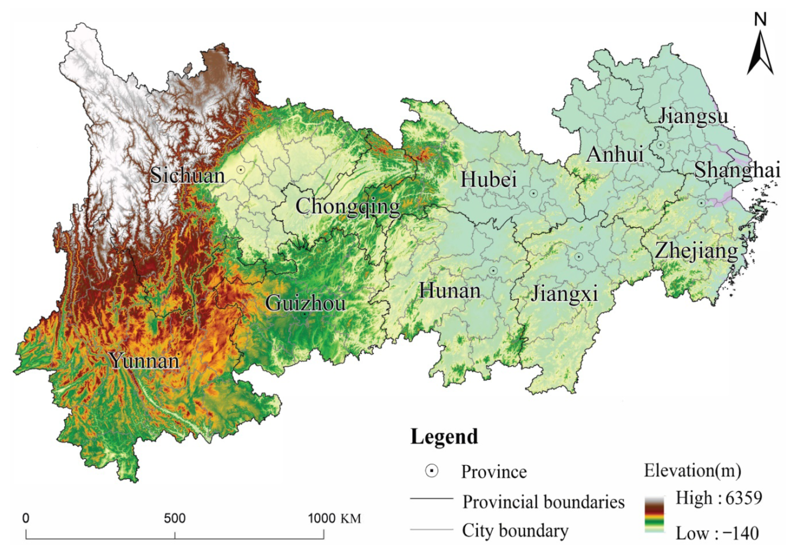
The study area, the Yangtze River Economic Belt, is situated within the Yangtze River Basin of China. It covers 11 provinces and cities, including Shanghai, Jiangsu, Zhejiang, Anhui, Jiangxi, Hubei, Hunan, Chongqing, Sichuan, Yunnan, and Guizhou, as depicted in Figure 1. The total study area is approximately 2.05 million square kilometers, and its population and GDP account for about 40% of China’s total. With the rapid development of the economy and society, the study area has recently encountered serious challenges related to ecological destruction and environmental deterioration. Given its vast geographical extent and substantial economic weight, the study area occupies a strategically critical position in advancing China’s overarching environmental sustainability agenda. Moreover, environmental stress within this region carries implications that extend well beyond its administrative boundaries, potentially affecting the ecological security of the broader Yangtze River Basin and beyond.
To strengthen coordinated development, the Outline of the Yangtze River Economic Belt Development Plan, released in 2016, emphasizes the development model focusing on ecological and green civilization. The development plan underlines sustainable development in social, economic, and environmental aspects, aligning with the goals of the 2030 Agenda for Sustainable Development. Considering its immense economic scale, severe ecological pressures, and pivotal role in shaping China’s transition toward a greener growth model, this study identifies the Yangtze River Economic Belt as a priority region for examining sustainable environmental development.

2.2. Datasets and Preprocessing

Considering that the sustainable development values of similar years may not undergo significant changes, this study selected cross-sectional datasets from 2013, 2017, and 2021 at five-year intervals for the study area. The datasets were roughly divided into environmental datasets, geographical information datasets, and socialeconomic datasets. Environmental datasets were sourced from statistical yearbooks and remote sensing data production. The PM2.5 data with a spatial resolution of 0.01° was derived from the Atmospheric Composition Analysis Group (https://sites.wustl.edu/acag/datasets/surface-pm2-5/ (accessed on 22 July 2024)). The O3 data, with a spatial resolution of 1 km, was downloaded from the Giovanni platform (https://giovanni.gsfc.nasa.gov/giovanni/ (accessed on 18 August 2024)). The normalized difference vegetation index (NDVI) data with a resolution of 1 km was retrieved from the EARTHDATA platform (https://www.earthdata.nasa.gov/ (accessed on 29 August 2024)). Other environmental data were collected from the statistical yearbook of each prefecture-level city in the study area. Four socialeconomic factors were selected in this study: population density (PD), per capita GDP (GDPpc), human activity disturbance (HAD), and urbanization rate (UR). PD, GDPpc, and UR data were directly obtained from a statistical yearbook. HAD data were derived by multiplying the disturbance grade index (listed in Table 1) by the weighted sum of the areas corresponding to different land use types.
To address missing statistical data with respect to the prefecture-level cities, spatial interpolation methods (e.g., Kriging and IDW) were applied to environmental and climate variables, whereas temporal interpolation was used for socioeconomic data, given their fundamentally different spatial dependencies. The accuracy of the interpolation results from different methods was first evaluated, and the interpolation method with the highest accuracy was selected to estimate the missing value. Meanwhile, considering that this study was conducted at the city scale, remote sensing data with a relatively high resolution were converted according to each prefecture-level city by spatial statistical aggregation.

3. Methodology

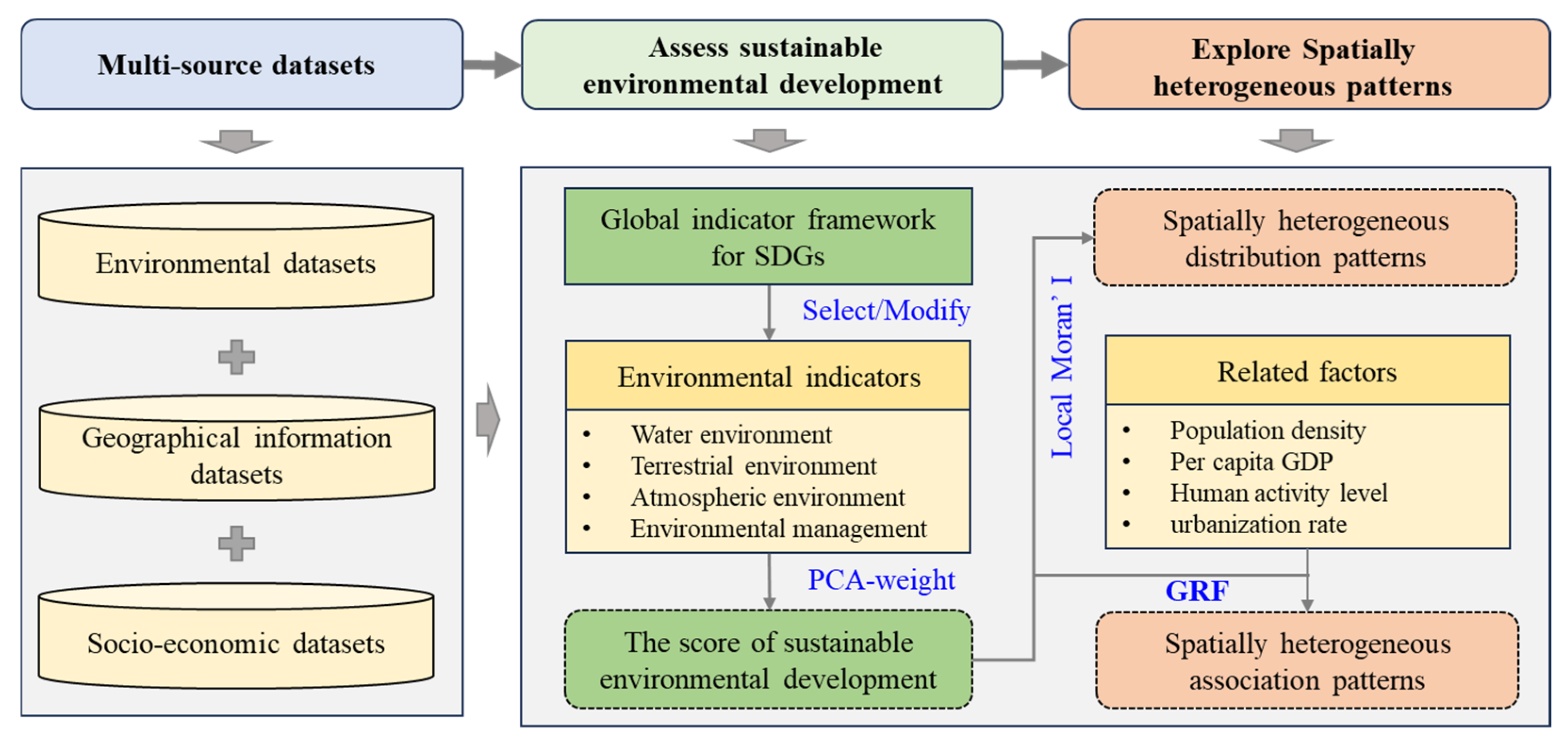
Figure 2 depicts the primary technical method for investigating spatially heterogeneous patterns of SED. Initially, SED status is determined by integrating environmental and geographical datasets. Specifically, within the context of the Global Indicator Framework for the Sustainable Development Goals (SDGs), environment-related indicators are selected or modified. This study identifies four distinct categories of environmental indicators: water environment, terrestrial environment, atmospheric environment, and environmental management. To account for the intercorrelation among these indicators, a weight calculation utilizing principal component analysis (PCA-weight) is employed to determine SED scores. The method is detailed in Section 3.1.
Spatially heterogeneous patterns are categorized into two types: spatially heterogeneous distribution patterns and spatially heterogeneous association patterns. The former focuses on understanding the spatial variations in SED across the entire study area, utilizing spatial statistical methods such as Moran’s I, which is introduced in Section 3.2. The latter seeks to reveal the relationships between SED and related factors that vary spatially. For this purpose, geographically weighted random forest (GRF) is employed, which is introduced in Section 3.3.

3.1. Assessing Sustainable Environmental Development Based on Standardized Weighted Indices

Within the Global Indicator Framework for evaluating SDGs, a total of 230 indicators have been chosen to monitor 17 integrated and indivisible goals. These indicators are presented at the global scale. However, due to regional variations in geographical location and spatial scale, significant challenges persist in applying these indicators to assess SDG progress at provincial or municipal levels. For instance, some indicators lack universally accepted statistical definitions, while others do not align with local data selection criteria at these administrative levels [24]. The global SDG indicator framework has been developed with 231 indicators, yet approximately 17% of these indicators have limited applicability to certain countries or regions due to geographical features or unique national contexts [25]. Moreover, widespread data gaps continue to hinder the accurate assessment of SDG performance across countries and goals, with the average data missing rate across all countries reaching approximately 50% [26].
These challenges also exist in the SED assessment. Data gaps and the limited regional applicability of certain indicators are well-recognized challenges in sustainability assessment, as comprehensive evaluation results are often constrained by either data unavailability or the inapplicability of certain indicators to specific local contexts [27]. Therefore, considering the above challenges, 14 indicators covering five SDGs are selected to assess SED progress in prefecture-level cities, as depicted in Table 2.
To ensure comparability across diverse indicators, it is essential to implement indicator standardization that transforms the raw data of each indicator into dimensionless values within a uniform range [12,15,28]. In this study, the standardization range is set from 0 to 100. A lower standardized indicator value means better performance, whereas a higher value corresponds to better performance. Lower- and upper-bound parameters are critical in the standardization process, which are identified by reference to national or local standards and the 2018 SDG Index and Dashboards Report. For indicators without a reference, the upper and lower bounds are determined by the average value of five top-performing units and 2.5% of the average. Subsequently, the standardized indicator S n o r ( i ) can be defined as
S n o r ( i ) = S ( i ) S l b ( i ) S u b ( i ) S l b ( i ) × 100 %
where S ( i ) represents the initial score of indicator i; S l b and S u b denote the upper- and lower-bound parameters of indicator i, respectively. If S ( i ) exceeds the upper (lower-)-bound parameter, then S n o r ( i ) is set at 100 (0).
These standardized indicators describe SED from multiple perspectives, and their aggregation yields the overall SED score. Given the potential correlations among indicators, principal component analysis (PCA) is first applied to determine indicator weights. This method derives the weight of each indicator based on its contribution to the principal components that account for the majority of the total variance. Specifically, indicators with higher loadings on the first several principal components receive greater weights, as they contribute more to explaining the underlying variability in the original dataset. To ensure cross-year comparability, we applied PCA to the pooled panel data across all three periods to derive a fixed factor loading matrix. This unified matrix is then used to calculate SEDI scores for each year, ensuring that temporal variations reflect actual changes in SEDI rather than shifts in the weighting structure. Subsequently, the weighted mean value of these standardized indicators is defined as the overall score of the sustainable environmental development index (SEDI)::
S E D I = 1 n k = 1 n W ( k ) S n o r ( k )
where W ( k ) represents the weight of the indicator k, and n denotes the total number of indicators used to compute SEDI.

3.2. Identifying Spatially Heterogeneous Distribution Patterns Using Local Moran’s I

Spatially heterogeneous distribution patterns refer to spatial differentiation over time. Spatial differentiation characterizes the local characteristics of spatial autocorrelation or dependency in SED status. In spatial statistics, Moran’s I index is utilized to measure spatial autocorrelation or dependency. Because it uses a global value to reveal the overall characteristics of spatial autocorrelation, the global Moran’s I index is not suitable for detecting spatial differentiation. Consequently, the local Moran’s I, a variant of Moran’s I, is an effective index for modeling spatial differentiation [29]. In this study, the local Moran’s I index is used to identify spatially heterogeneous distribution patterns.
For geographic unit j, the local Moran’s I is defined as follows:
I j = n ( y j y ¯ ) k = 1 n w j k ( y k y ¯ ) k = 1 n ( y k y ¯ ) 2
where m represents the number of geographic units; x j is the SED score for geographic unit j; y ¯ is the average value across all the units; w j k is the spatial weight matrix between units j and k, which takes a value of 1 when the two units are neighbors (sharing a boundary or vertex) and 0 when they are not. The local Moran’s I value ranges from −1 to 1. The local Moran’s I is tested using a normal Z statistic:
Z ( I j ) = I j E ( I j ) V a r ( I j )
where E ( I j ) and V a r ( I j ) represent the expectation and variance of the local Moran’s I, respectively. A value of |Z| exceeding 1.65 at a 0.05 confidence level indicates the rejection of the null hypothesis, suggesting the presence of spatial autocorrelation. When the I j value is greater than 0, spatial autocorrelation is positive between unit i and its adjacent units, which corresponds to a “high–high” pattern for ( y j y ¯ ) > 0 or a “low–low” pattern for ( y j y ¯ ) < 0 within the local area. Otherwise, spatial autocorrelation is negative and a “low–high” pattern for ( y j y ¯ ) > 0 or a “high–low” pattern for ( y j y ¯ ) < 0 patterns can be distinguished.

3.3. Exploring Spatially Heterogeneous Association Patterns Using Geographical Random Forests

A key scientific question underlying this study is that the relationships between socioeconomic factors and SED status may vary across space—that is, spatial non-stationarity exists in these relationships. To explicitly model spatial non-stationarity, this study employs geographical random forest (GRF), which extends the conventional random forest algorithm by incorporating spatial heterogeneity into the modeling framework. Specifically, it calibrates a separate local random forest model at each data location using a spatial kernel weighting scheme, allowing the relationships between driving factors and SED to vary continuously across space, thereby capturing spatially non-stationary effects [30,31]. The fundamental principle of GRF is consistent with geographically weighted regression (GWR), which aims to establish a series of local linear regression models to describe the spatially varying relationships among variables [32]. As with GWR, the principle of GRF can be succinctly expressed through a regression formula as follows:
y j = R F i ( x j ) + e j
where y j and x j are the output variable and input variables, respectively; e j is the error term; and R F j ( ) refers to the local RF model at geographic unit j constructed using nearby observations [33,34].
Unlike global models (e.g., standard random forest), which inherently assume spatial stationarity, our study employs the GRF to explicitly capture potential spatial non-stationarity in socioeconomic–SED relationships. To statistically validate the necessity of this local modeling approach, we conduct a permutation test where the null hypothesis ( H 0 ) posits that the spatial relationship is stationary (homogeneous). Under H 0 , the specific geographic arrangement of samples should not dictate model performance.
To test this, we construct a statistic based on prediction accuracy by randomly permuting the spatial locations of the observations while keeping the attribute values fixed. If spatial heterogeneity truly prevails, disrupting the spatial structure via permutation should significantly degrade the GRF model’s performance (i.e., increase prediction errors). Accordingly, a statistical value p is defined as follows:
p = k = 1 T I k / T ,
where T represents the total number of permutation iterations. I k is an indicator variable determined by comparing the mean squared error (MSE) of the real dataset, denoted as MSE ( r ) , with that of the k -th permuted dataset, MSE ( k ) . Specifically, if MSE ( r ) > MSE ( k ) , then I k = 1 ; otherwise, I k = 0 . Consequently, if the calculated p -value is lower than the significance level (e.g., 0.05), the null hypothesis is rejected, confirming that the relationships among variables exhibit significant spatial non-stationarity.
Further, in traditional random forests, the importance of an independent variable is typically assessed using the out-of-bag error, which is commonly measured as an increase in the mean squared error (iMSE). Since each random forest model in GRF is constructed at every data location, the importance of each independent variable within each sub-model can be determined to investigate spatially heterogeneous association patterns among variables. Moreover, to explicitly capture the directional effects of individual predictors prior to examining their spatial variations, we supplement the global random forest model with SHAP (SHapley Additive exPlanations) values. Unlike conventional importance metrics that merely quantify the magnitude of influence, SHAP values provide signed contributions for each feature, thereby revealing whether a factor exerts a positive or negative influence on the response variable at the global scale [35].

4. Results

4.1. Spatial Characteristics of Sustainable Environmental Development

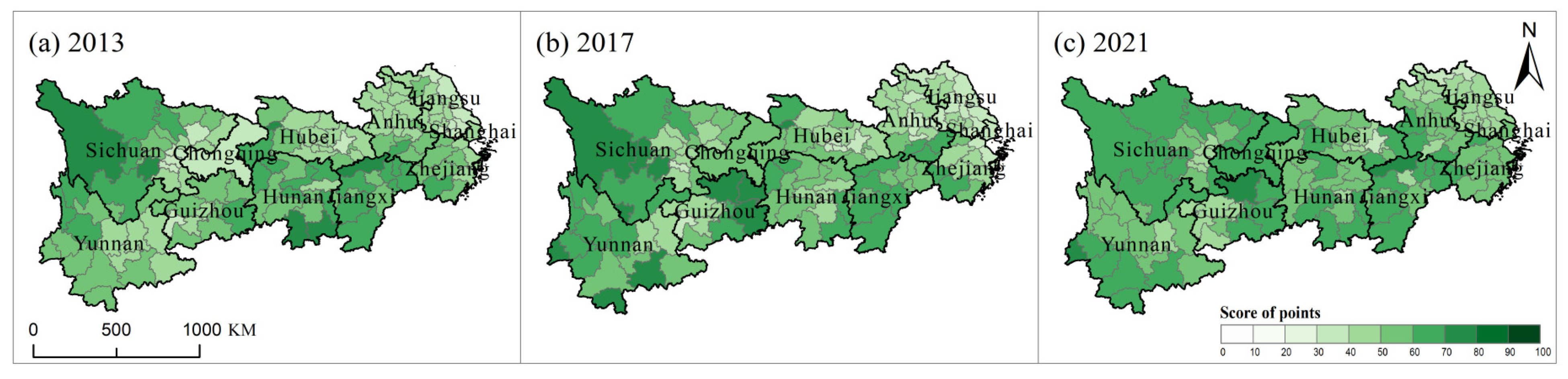
The spatial distribution of SEDI scores is shown in Figure 3. Scores range from 0 to 100, with darker shades indicating higher index values and lighter shades indicating lower values. In 2013, regions with low SEDI scores below 40 were predominantly found in Jiangsu, Anhui, and Hubei provinces, as well as the city of Chongqing. By 2017 and 2021, these areas experienced varying degrees of improvement, with Chongqing demonstrating particularly significant progress in SED. Conversely, cities like Guizhou and Yunnan exhibited relatively high SEDI values exceeding 60, which remained relatively stable across the three-year period.
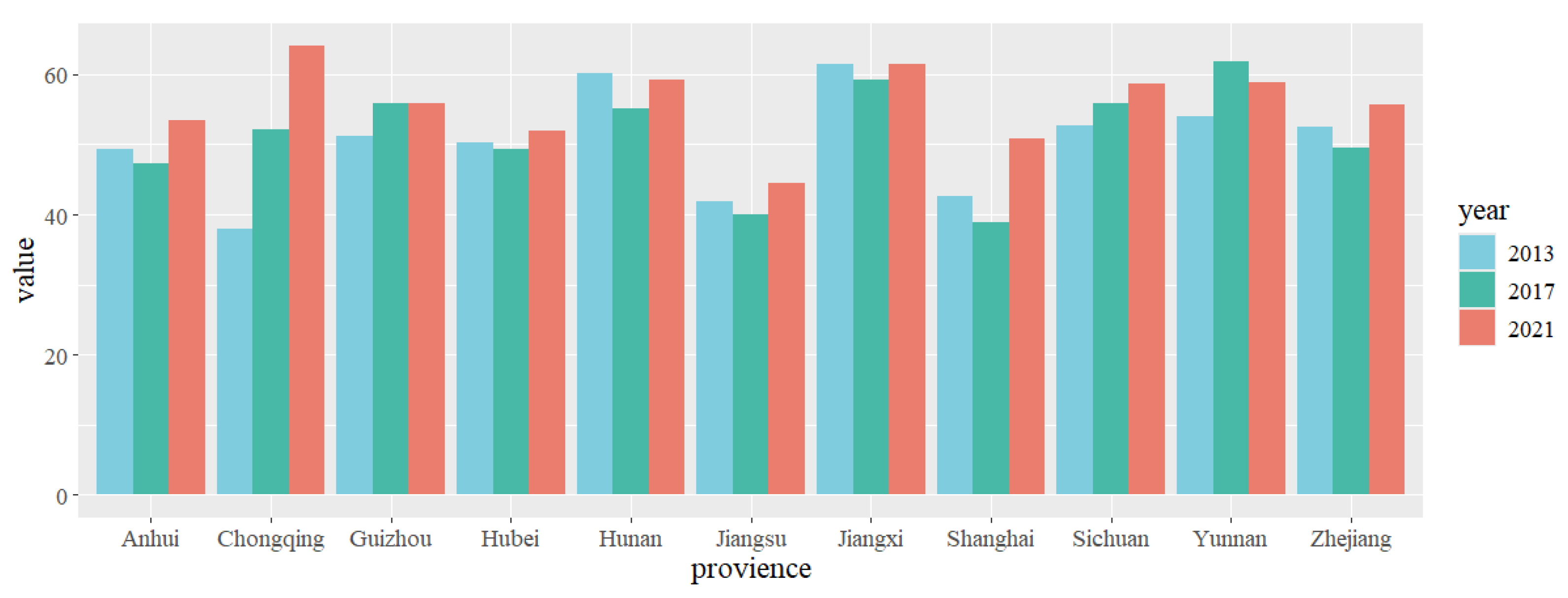
Figure 4 presents the statistical results of SEDI scores for each province within the study area. It reveals that, at the provincial level, nearly all SEDI scores were below 60 across the three observed periods. On a broader scale, the scores from 2013 to 2021 show an upward trend, with the 2021 scores typically exceeding those of 2013. Notably, seven prefecture-level cities exhibited a downward trend in 2017.
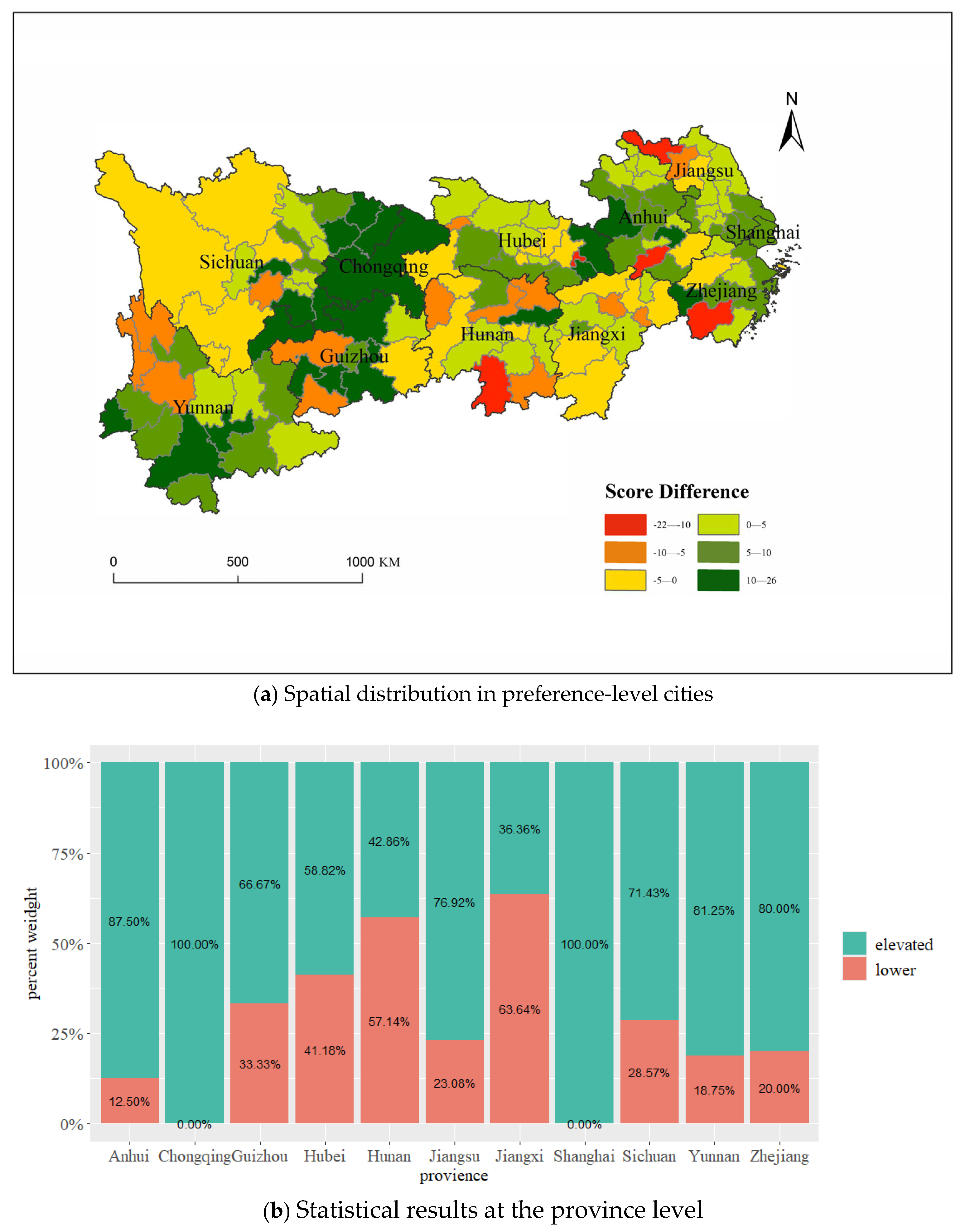
To assess the dynamic SED evolution from 2013 to 2021, the change in SEDI scores between 2021 and 2013 was computed. A positive difference indicates progress in SED, whereas a negative difference suggests ongoing challenges. Figure 5 shows the spatial distribution of these changes and the province-level statistical results. Approximately 68.4% of cities within the Yangtze River Economic Belt showed improved scores. In Anhui, Yunnan, and Zhejiang Provinces, cities with improved scores accounted for over 80% of the total, whereas in Jiangxi and Hunan Provinces, this figure did not exceed 50%.

4.2. Spatially Heterogeneous Patterns of Sustainable Environmental Development

4.2.1. Spatial Autocorrelation Patterns of Sustainable Environmental Development

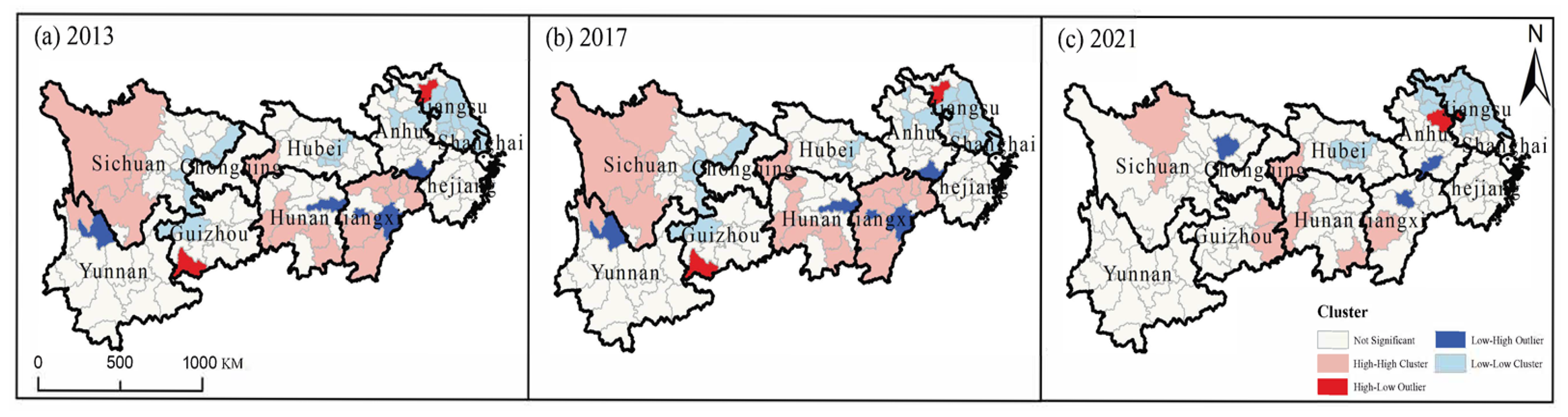
The global Moran’s I values for the three years were 0.42, 0.49, and 0.39, respectively, all statistically significant at the p < 0.01 level. These results indicate a moderate but statistically significant positive spatial autocorrelation of SED across the study region, suggesting a consistent tendency toward spatial clustering over the study period. Spatially heterogeneous distribution patterns of the SEDI scores were then identified using the local Moran’s I, as depicted in Figure 6. In 2013, high–high clusters were predominantly found in prefecture-level cities across Sichuan, Jiangxi, and Hunan Provinces, while low–low clusters were mainly concentrated in Shanghai, Jiangsu, and Sichuan Provinces, with scattered areas in Guizhou and Chongqing. Abnormal areas were noted, with low–high outliers primarily located in Jiangxi and its neighboring prefecture-level cities in Anhui and Hunan. Two high–high outlier areas were detected in Guizhou and Jiangsu Provinces. By 2017, these spatial patterns remained largely unchanged, except for the expansion of high–high clusters in Jiangxi Province. In 2021, significant changes occurred, with a reduction in the extent of all spatial patterns. High-value clustering areas in Jiangxi, Sichuan, and Hunan decreased, and low-value clustering areas were absent in Sichuan and Guizhou Provinces. The number of abnormal areas diminished, and their distribution shifted to neighboring regions.

4.2.2. Evaluation Results of the GRF Model’s Performance

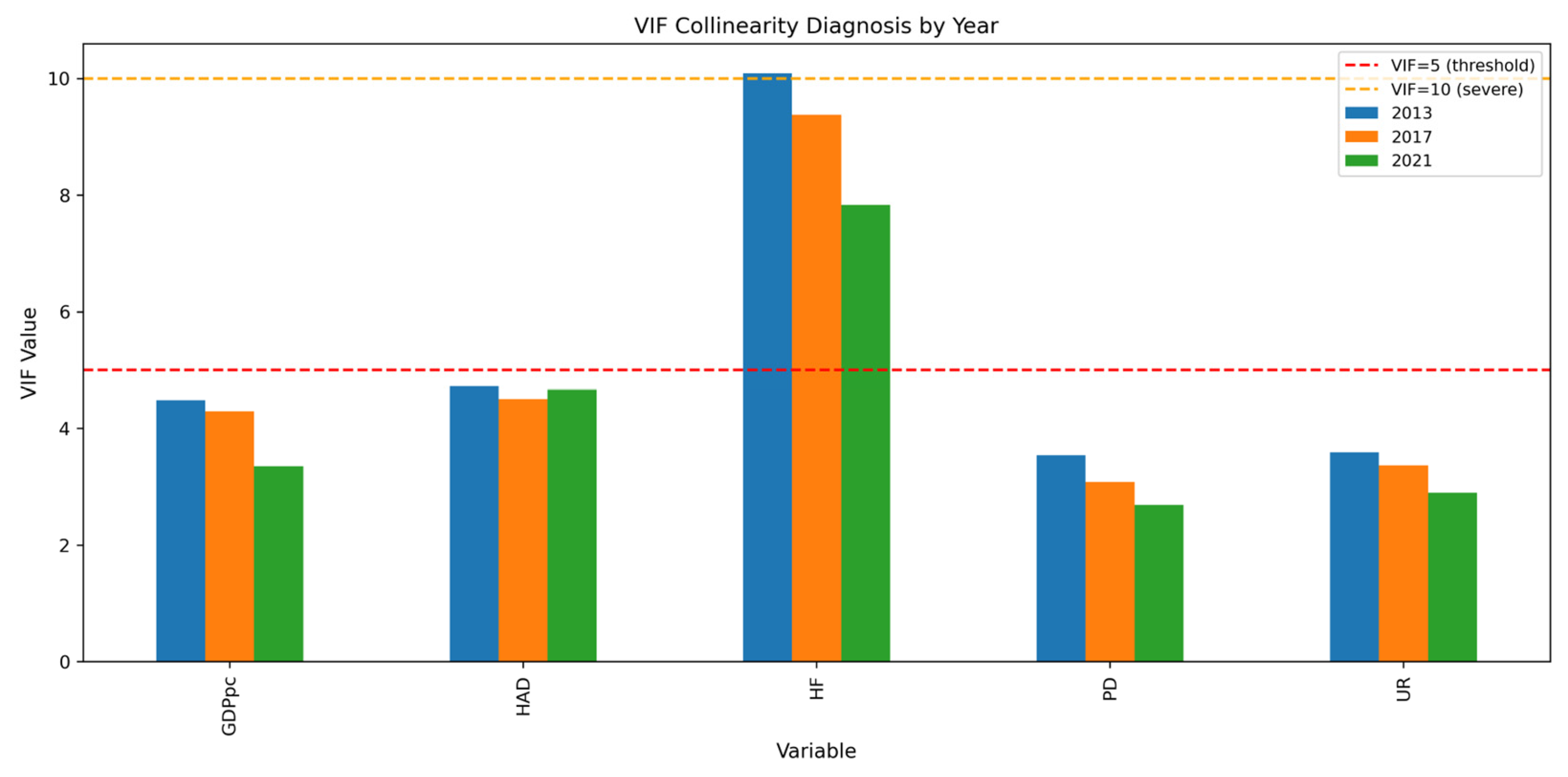
As previously mentioned, the geographical random forest (GRF) was employed to investigate the association patterns between SED and related factors. In the regression model, the SEDI scores served as the output variable, with input variables including human footprint (HF), population density (PD), per capita GDP (GDPpc), human activity disturbance (HAD), and urbanization rate (UR). Through VIF collinearity diagnosis, as shown in Figure 7, it is evident that HF consistently exhibits severe multicollinearity across all years, with VIF values far exceeding the threshold and other variables. Therefore, the HF variable should be removed to ensure the reliability and stability of the regression model.
Optimal hyperparameters for the geographically weighted random forest (GRF) model were identified via grid search with 5-fold cross-validation. For the spatial weighting component, three kernel functions (bi-square, Gaussian, and triangular) were evaluated with a global fixed bandwidth, where candidate bandwidths ranged from the 10th to 50th percentiles of the pairwise distance matrix at 5% intervals, and the optimal combination was chosen by maximizing the average cross-validated R2. For the number of trees (n_estimators), we examined candidate values of {100, 200, 300, 400, 500, 600, 800, 1000} and selected the minimum count at which the cross-validated R2 converged to a stable level, thereby balancing computational efficiency and prediction performance. Other hyperparameters were assigned default values recommended by the canonical RF and GRF literature [31].
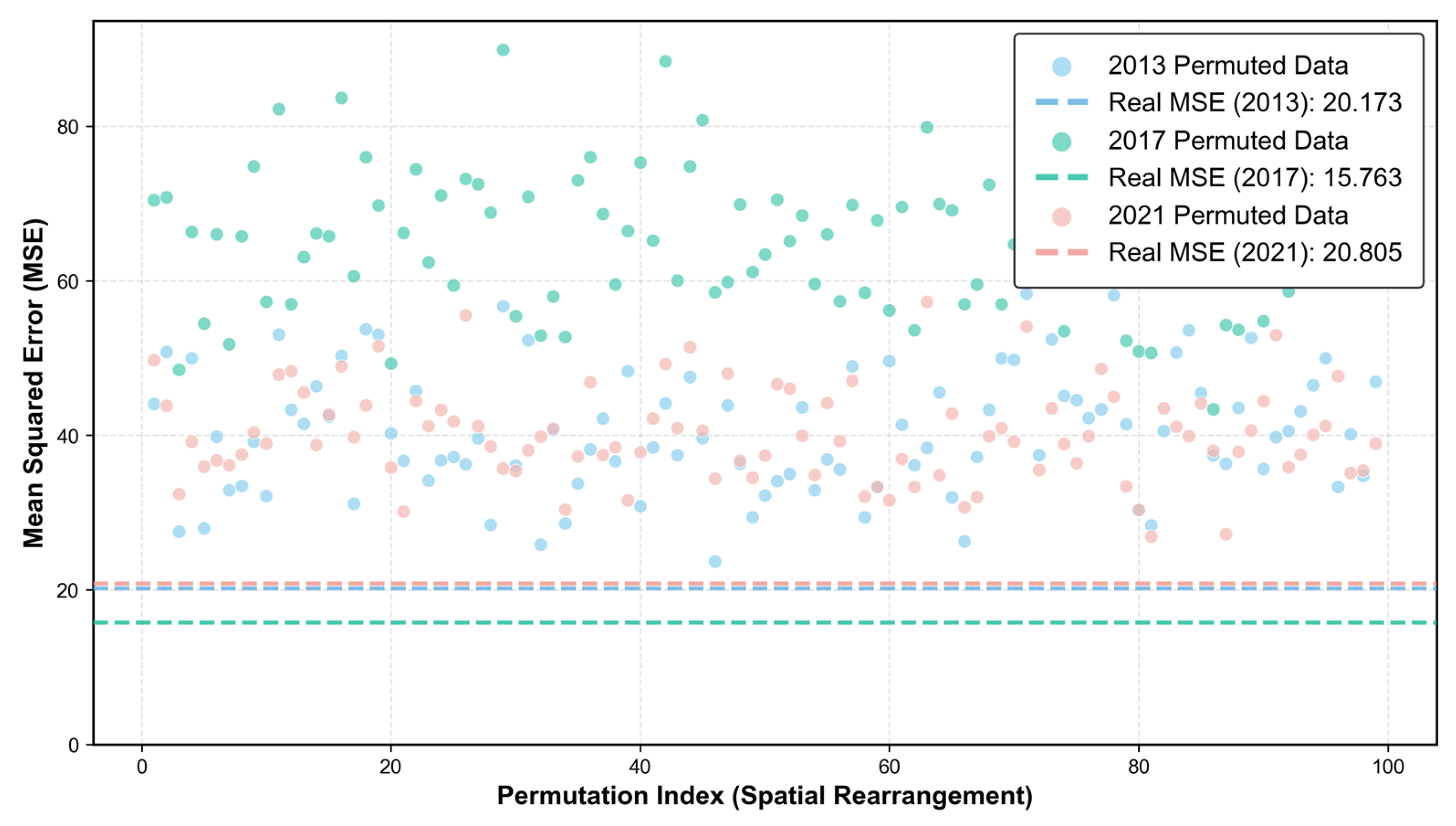
To assess the effectiveness of the GRF, we compared its performance with that of random forest (RF) and geographically weighted regression (GWR) models. The evaluation results, including the MSE and coefficient of determination (R2), are presented in Table 3. The GRF model yielded R2 values of 0.769, 0.867, and 0.712 across the three periods, respectively, all of which were higher than those of the RF and GWR models in the corresponding periods. Furthermore, the MSE values for the GRF were 20.173, 15.763, and 20.805 for the three years, all of which were lower than the MSE values of the RF and GWR models. This demonstrates that the GRF is superior to both the RF and GWR in capturing relationships between SED and associated factors. Meanwhile, to validate the necessity of employing the GRF model, we conducted a permutation test with 99 iterations. The results show that the p-value is 0.00, which is well below the 0.05 significance level. Therefore, the null hypothesis (H0) of spatial stationarity is rejected, confirming that the relationships between socioeconomic factors and SED exhibit significant spatial non-stationarity. This finding justifies the use of a local modeling approach (i.e., GRF) over global models that assume homogeneous relationships across space.
The results of the statistical test for spatial non-stationarity are presented in Figure 8. For each of the three study years, the GRF model was fitted to 999 randomly permuted datasets, generating a null distribution of the mean squared error (MSE) under the assumption of spatial stationarity (i.e., the null hypothesis). In all cases, the MSE obtained from the actual (unpermuted) data was substantially lower than that from every permuted replicate. Consequently, following Equation (6), the empirical p-value was computed as zero, leading to the rejection of the null hypothesis at the conventional significance level. This finding provides strong statistical evidence that spatial non-stationarity exists persistently across all three years, further corroborating the validity and necessity of employing the GRF model in this study.

4.2.3. Spatially Heterogeneous Associations Between Driving Factors and SED

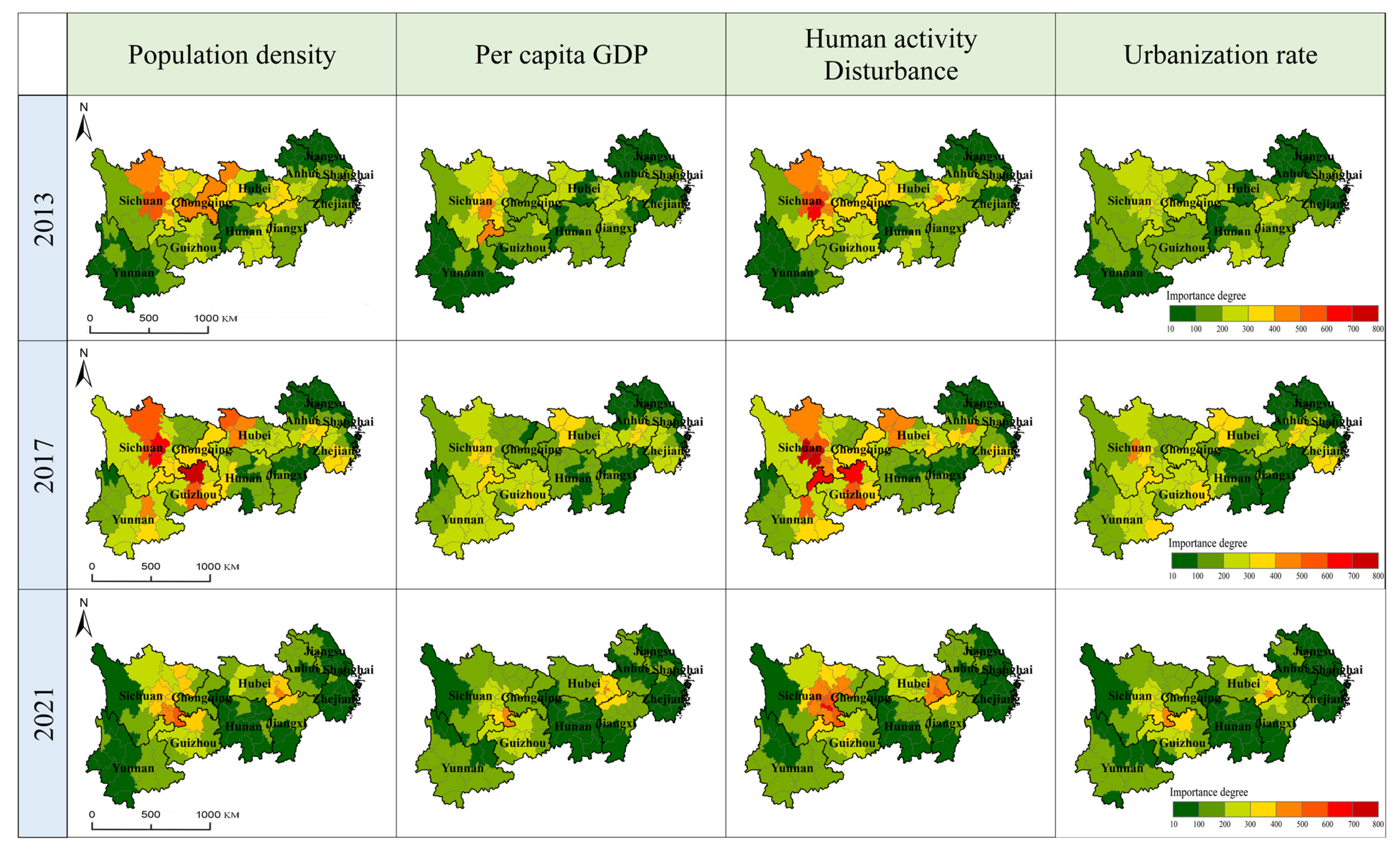
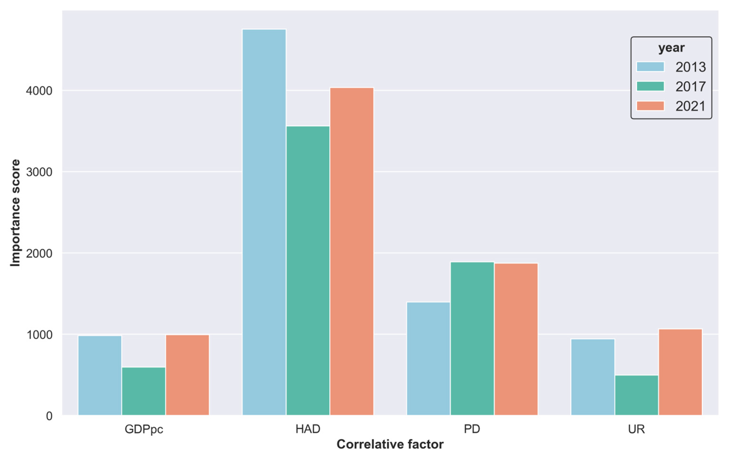
Based on the constructed GRF model, the importance of the independent variable can be computed. The global importance is shown in Figure 9. In 2013, the importance of human activity disturbance (HAD) was the highest, followed by population density (PD), per capita GDP (GDPpc), and urbanization rate (UR). Subsequently, in 2017, the importance of all variables increased. In particular, the impact of human activity disturbance and population density showed a significant increasing trend. In 2021, all factors had a reduced impact on SED and were less important than those in 2013, but human activity disturbance and population density still had the greatest impact on SED. This temporal decline in HAD and PD importance after 2017 may reflect the delayed effects of environmental policy interventions, which gradually restructured local industrial composition and labor dynamics, thereby attenuating the marginal contribution of these anthropogenic pressures on SEDI [36]. According to the SHAP values, HAD, PD, and GDPpc each exhibited a positive directional influence on SEDI over the three study years, whereas UR showed a negative influence. This indicates that, during this period, higher levels of agricultural development, population density, and economic output tended to be associated with increased SEDI, while higher urbanization rates were associated with decreased SEDI.
Figure 10 illustrates the spatial variation in the impact of the related factor on the SED. In 2013, prefecture-level cities in Sichuan, Chongqing, and Hubei Provinces exhibited a significant influence of population density on the SED. This influence was particularly pronounced in these regions and their surrounding cities, which saw a gradual increase in importance between 2013 and 2017. However, by 2021, this importance had notably diminished. The importance degree of human activity disturbance exhibited a consistent spatial distribution pattern with that of population density during these three periods. This spatial heterogeneity may reflect the divergent trajectories of industrial restructuring along the Yangtze River Basin: While downstream municipalities achieved environmental gains primarily through advances in clean production technologies, their midstream and upstream counterparts adopted strategies centered on restricting polluting industries. Such differential policy pathways have generated location-specific responses in how population concentration and anthropogenic disturbance affect environmental sustainability [36,37].
Per capita GDP consistently influenced the SED in both local and global analyses, with lower levels observed across all three years. From 2013 to 2017, the scope of regions experiencing relatively higher impact narrowed, while the significance of per capita GDP rose in certain cities within Hunan, Yunnan, and Hubei Provinces. By 2021, per capita GDP exerted a reduced impact in most regions, except for cities bordering Hubei and Jiangxi Provinces, as well as those in Sichuan and its neighboring prefecture-level cities. This pattern may be associated with the spatial evolution of industrial transfer, where the initial phase of relocation into central provinces heightened economic pressures on local environmental capacity before gradual adaptation occurred.
In 2013, the urbanization rate’s influence on SED was generally low across most prefecture-level cities, except for certain cities in Hubei and Sichuan Provinces, which exhibited a higher impact. By 2017, this influence rose in most cities within Yunnan, Guizhou, and Zhejiang Provinces, only to decline once more in 2021, except for the eastern portion of Hubei Province and the southeastern region of Sichuan Province. This fluctuating pattern of UR importance reflects the inherent tensions in China’s urban sustainability transition: as metropolitan areas became progressively decoupled from ecological systems through technology-driven development, the environmental burden of urban expansion escalated, yet the additional explanatory power of urbanization rates for environmental outcomes grew increasingly dependent on localized industrial profiles and the enforcement of environmental standards [38,39].

5. Discussion

Previous sustainable development assessment studies have predominantly focused on the 2030 Sustainable Development Goals. These assessments are typically based on the United Nations’ SDGs or targets and utilize the 2030 SDG Global Indicator Framework [9,17]. Indeed, sustainable development essentially involves three core dimensions: environment, economy, and society. Therefore, evaluating sustainable development from the perspective of a unified theme related to various goals or targets can provide a more comprehensive picture of the overall development of the theme. Consequently, this study chooses the environment as the theme and aims to investigate the spatially heterogeneous patterns of SED in prefecture-level cities within the Yangtze River Economic Belt, China.
The selection of appropriate indicators and the acquisition of relevant data represent significant challenges in evaluating SED. The 2030 SDG Global Indicator Framework is typically constructed at the national scale, rendering the indicators inapplicable at the provincial or prefecture-level city scale [13]. Given the difficulty in obtaining comprehensive data at the prefecture level, a total of 14 indicators covering 10 SDGs were selected to construct the SEDI. The results indicate that the SEDI scores generally trended upward across most cities over the three observed periods. Comparing scores from 2013 and 2021, approximately 70% of cities demonstrated improved scores. Notably, because ecological and green civilization has been promoted as a national development model since 2016, emphasizing the protection of the ecological environment while developing the economy is likely to promote overall SED improvement.
However, there were still some prefecture-level cities with a downward trend, especially in most cities of Jiangxi, Hubei, and Hunan Provinces. The slower improvement or decline of SEDI in Jiangxi, Hubei, and Hunan can be attributed to three main factors: (1) a heavy industrial structure dominated by high-energy-consumption sectors, which imposes higher environmental compliance costs [40]; (2) insufficient green innovation capacity and R&D investment compared to eastern provinces like Jiangsu [41]; (3) weaker inter-regional coordination mechanisms that limit the effectiveness of environmental policies [42]. These structural constraints have hindered these provinces from achieving the same level of environmental improvement as their eastern counterparts.
Using local Moran’s I to detect spatially heterogeneous distribution patterns, the number of high–high and low–low clusters decreased by 2021. Through period-by-period comparisons, it was confirmed that the reduction was driven by regional convergence (narrowing inter-regional disparities) rather than increased spatial randomness. This finding aligns with documented convergence patterns in China’s environmental and sustainability research [43,44], where significant β-convergence and spatial spillover effects have been identified across provinces. The convergence interpretation is further supported by evidence of spatial shifts in industrial pollution from “high in the east, low in the west” toward national convergence [45], mirroring the trend observed in our SEDI analysis.
Geographically random forest (GRF) was employed to investigate the association between SED and its potential drivers. Compared to conventional geographically weighted regression and standard random forest, GRF offers the advantage of simultaneously accommodating complex non-linear relationships and spatial heterogeneity among variables—a capability that is critical given that environmental responses to socioeconomic stressors are rarely uniform or linear across space [46,47]. Model performance evaluations confirmed the presence of both non-linearities and spatial variations in the factor–SED relationships across the study area, justifying the application of this localized modeling framework. Importantly, by incorporating interpretable machine learning techniques, we were able to quantify spatially varying variable importance, thereby moving beyond global-rank descriptions to reveal how the influence of each driver changes across geographic contexts.
Globally, human activity disturbance (HAD) and population density (PD) consistently outperformed per capita GDP and urbanization rates in explaining SED variation across all three periods. This predominant role of anthropogenic pressure indicators can be attributed to the direct and localized nature of their environmental impacts—unlike macroeconomic or urbanization proxies, which often manifest with time lags and through indirect pathways, human activity intensity and population concentration exert immediate pressures on resource consumption, waste generation, and habitat modification [26,48]. Spatially, cities with high HAD and PD importance were predominantly concentrated in Sichuan, Chongqing, Guizhou, and Hubei Provinces, where rapid urbanization and industrial agglomeration have intensified the coupling between human activities and environmental systems [49]. Notably, the spatial distribution patterns of HAD and PD importance were found to be highly consistent, suggesting that population agglomeration serves as a primary carrier through which anthropogenic disturbances translate into environmental outcomes—a finding consistent with the population–environment interaction framework proposed in recent sustainability research [50].
These spatially explicit results underscore the necessity of place-based policy interventions: In high-impact regions—particularly those where HAD and PD importance consistently ranked highest across all three periods—managing human activity intensity and optimizing population distribution may yield more immediate SED improvements than broad-based economic or urbanization policies. Specifically, for cities in Sichuan, Chongqing, Guizhou, and Hubei, where the influence of anthropogenic pressure on environmental outcomes was most pronounced, policy efforts should prioritize localized interventions such as regulating industrial emission intensity, improving urban land use efficiency, and guiding population agglomeration toward environmentally sustainable spatial configurations. Conversely, in regions where GDPpc and UR exhibited relatively higher importance, policy design should focus on promoting green technological innovation and improving the environmental performance of urban expansion. This spatially differentiated strategy, as opposed to a one-size-fits-all approach, is likely to be more effective in enhancing SED across diverse regional contexts.
Nonetheless, this study presents certain limitations. Firstly, this study adopts a data-driven approach to selecting indicators for SED evaluation, focusing on those with readily accessible supporting data for evaluating environmental sustainability. In fact, some environment-related indicators have been ignored, which may directly affect the effectiveness of the evaluation. Moreover, the use of simple weighting schemes, while methodologically straightforward, may fail to capture the differential importance of individual indicators and could introduce subjective bias into the aggregation process. Therefore, how to indirectly obtain or estimate data to comprehensively evaluate SED, as well as how to develop more sophisticated weighting methods that better reflect indicator priority, represents a significant area for future research. In addition, although a geographical random forest was used to effectively explore the spatially heterogeneous association patterns between SED and related factors, the relative importance of features from the geographical random forest does not clearly elucidate the impact mechanism. Consequently, a more detailed exploration of the relationship—particularly accounting for spatial heterogeneity and nonlinearity—also warrants further investigation.

6. Conclusions

This study proposes a framework for exploring spatially heterogeneous patterns of sustainable environmental development. This framework consists of two components: the assessment of sustainable environmental development using the 2030 Sustainable Development Goal (SDGs) Global Indicator Framework and the exploration of the relationship between SED and related factors. The framework was applied to evaluate SED in the Yangtze River Economic Belt, China. The principal findings can be summarized as follows: The SED exhibited a positive trend in most cities during these three periods. From 2013 to 2021, approximately 70% of the cities demonstrated an upward trend. However, some prefecture-level cities, particularly in Jiangxi, Hubei, and Hunan provinces, exhibited a downward trend. The number of high–high and low–low clusters decreased from 2013 to 2021, indicating that SED in neighboring regions generally exhibited distinct change characteristics. SED and its related factor exhibited non-linear relationships, with these relationships varying spatially across the study area. The spatial distribution of the impact of human population activity and population density on the sustainable environment was consistent. Cities experiencing a high impact were predominantly located in Sichuan, Chongqing, Guizhou, and Hubei provinces.

Author Contributions

Conceptualization, S.F.; methodology, H.L.; software, K.M.; validation, S.F., X.M., and H.L.; formal analysis, K.M.; investigation, S.F.; resources, H.L.; data curation, X.M.; writing—original draft preparation, H.L.; writing—review and editing, S.F.; visualization, K.M.; supervision, X.M.; project administration, H.L.; funding acquisition, S.F. All authors have read and agreed to the published version of the manuscript.

Funding

This research is supported by the Fujian Provincial Scientific Research Project for Young and Middle-aged Teachers (Science and Technology Category) (JAT220324); the Horizontal Research and Development Project of Minjiang University (2025MHX392); the Hunan Provincial Key Laboratory of Service Computing and Novel Software Service Technology, Hunan University of Science and Technology (E22502); and the K-2023 Principal’s Fund: Research on Fast Screening Method and Application of Imaging Data Based on Information Entropy.

Institutional Review Board Statement

Not applicable.

Informed Consent Statement

Not applicable.

Data Availability Statement

Data will be made available upon request.

Conflicts of Interest

The authors declare no conflicts of interest.

References

  1. Verdejo, Á.; Espinilla, M.; López, J.L.; Melguizo, F.J. Assessment of sustainable development objectives in Smart Labs: Technology and sustainability at the service of society. Sustain. Cities Soc. 2021, 77, 103559. [Google Scholar] [CrossRef] [Scilit]
  2. Miao, Y.; Guo, J.; Liu, S.; Zhao, C.; Li, X.; Zhang, G.; Wei, W.; Ma, Y. Prediction of hourly PM2.5 using a space-time support vector regression model. Atmos. Environ. 2018, 181, 12–19. [Google Scholar] [CrossRef] [Scilit]
  3. Zeng, K.; Duan, X.; Chen, B.; Jia, L. Spatiotemporal Heterogeneity of Eco-Efficiency of Cultivated Land Use and Its Influencing Factors: Evidence from the Yangtze River Economic Belt, China. Sustainability 2025, 17, 3070. [Google Scholar] [CrossRef] [Scilit]
  4. United Nations. Transforming Our World: The 2030 Agenda for Sustainable Development. 2015. Available online: https://sdgs.un.org/ (accessed on 1 December 2022).
  5. Lin, B.; Ullah, S. Evaluating forest depletion and structural change effects on environmental sustainability in Pakistan: Through the lens of the load capacity factor. J. Environ. Manag. 2024, 353, 120174. [Google Scholar] [CrossRef] [Scilit] [PubMed]
  6. Lu, Y.; Nakicenovic, N.; Visbeck, M.; Stevance, A.-S. Policy: Five priorities for the UN Sustainable Development Goals. Nature 2015, 520, 432–433. [Google Scholar] [CrossRef] [Scilit] [PubMed]
  7. Maurice, J. Measuring progress towards the SDGs—A new vital science. Lancet 2016, 388, 1455–1458. [Google Scholar] [PubMed]
  8. Inter-Agency and Expert Group on SDG Indicators (IAEG-SDGs). Global Indicator Framework for the Sustainable Development Goals and Targets of the 2030 Agenda for Sustainable Development. 2017. Available online: https://unstats.un.org/sdgs/indicators/Global%20Indicator%20Framework%20after%202022%20refinement_Eng.pdf (accessed on 18 July 2019).
  9. Allen, C.; Metternicht, G.; Wiedmann, T. National pathways to the Sustainable Development Goals (SDGs): A comparative review of scenario modelling tools. Environ. Sci. Policy 2016, 66, 199–207. [Google Scholar] [CrossRef] [Scilit]
  10. D’adamo, I.; Gastaldi, M.; Imbriani, C.; Morone, P. Assessing regional performance for the Sustainable Development Goals in Italy. Sci. Rep. 2021, 11, 24117. [Google Scholar] [CrossRef] [Scilit] [PubMed]
  11. D’adamo, I.; Gastaldi, M. Sustainable Development Goals: A Regional Overview Based on Multi-Criteria Decision Analysis. Sustainability 2022, 14, 9779. [Google Scholar] [CrossRef] [Scilit]
  12. Tóthová, D.; Heglasová, M. Measuring the environmental sustainability of 2030 Agenda implementation in EU countries: How do different assessment methods affect results? J. Environ. Manag. 2022, 322, 116152. [Google Scholar] [CrossRef] [Scilit]
  13. Wei, D.; Li, W.; Yang, W.; Chen, H. Assessing the progress and spatial patterns of sustainable eco-environmental development based on the 2030 Agenda for SDGs in China. Int. J. Sustain. Dev. World Ecol. 2023, 30, 387–401. [Google Scholar] [CrossRef] [Scilit]
  14. Firoiu, D.; Ionescu, G.H.; Cismaș, L.M.; Vochița, L.; Cojocaru, T.M.; Bratu, R. Can Europe reach its environmental sustainability targets by 2030? A critical mid-term assessment of the implementation of the 2030 Agenda. Sustainability 2023, 15, 16650. [Google Scholar] [CrossRef] [Scilit]
  15. Schmidt-Traub, G.; Kroll, C.; Teksoz, K.; Durand-Delacre, D.; Sachs, J.D. National baselines for the Sustainable Development Goals assessed in the SDG Index and Dashboards. Nat. Geosci. 2017, 10, 547–555. [Google Scholar] [CrossRef] [Scilit]
  16. Yang, W.; Deng, M.; Tang, J.; Luo, L. Geographically weighted regression with the integration of machine learning for spatial prediction. J. Geogr. Syst. 2022, 25, 213–236. [Google Scholar] [CrossRef] [Scilit]
  17. Xu, Z.; Chau, S.N.; Chen, X.; Zhang, J.; Li, Y.; Dietz, T.; Wang, J.; Winkler, J.A.; Fan, F.; Huang, B.; et al. Assessing progress towards sustainable development over space and time. Nature 2020, 577, 74–78. [Google Scholar] [CrossRef] [Scilit] [PubMed]
  18. Wei, D.; Liu, B.; Duan, Z.; Yang, W. Measuring local progress of the 2030 Agenda for SDGs in the Yangtze River Economic Zone, China. Environ. Dev. Sustain. 2021, 24, 7178–7194. [Google Scholar] [CrossRef] [Scilit]
  19. Yang, P.; Zhang, X.; Hua, L. Analysis of Urban Ecological Quality Spatial Patterns and Influencing Factors Based on Remote Sensing Ecological Indices and Multi-Scale Geographically Weighted Regression. Sustainability 2023, 15, 7216. [Google Scholar] [CrossRef] [Scilit]
  20. Zhang, Q.; Shen, J.; Sun, F. Spatiotemporal differentiation of coupling coordination degree between economic development and water environment and its influencing factors using GWR in China’s province. Ecol. Model. 2021, 462, 109794. [Google Scholar] [CrossRef] [Scilit]
  21. Gan, X.; Du, X.; Duan, C.; Peng, L. Evaluation of ecological environment quality and analysis of influencing factors in Wuhan City based on RSEI. Sustainability 2024, 16, 5809. [Google Scholar] [CrossRef] [Scilit]
  22. Yang, J.; Huang, X. The 30m annual land cover dataset and its dynamics in China from 1990 to 2019. Earth Syst. Sci. Data 2021, 13, 3907–3925. [Google Scholar] [CrossRef] [Scilit]
  23. Ou, W.; Yang, R.; You, W. How Does the “Civilized City” Selection Affect Environmental Governance Performance? A Spatial DID Approach Based on Prefecture-Level Cities. Sustainability 2025, 17, 3812. [Google Scholar] [CrossRef] [Scilit]
  24. Vaidya, A.; Mayer, A.L. Use of the participatory approach to develop sustainability assessments for natural resource management. Int. J. Sustain. Dev. World Ecol. 2014, 21, 369–379. [Google Scholar] [CrossRef] [Scilit]
  25. ESCAP. Understanding SDG Data Gaps Based on National Realities. United Nations Economic and Social Commission for Asia and the Pacific. 2024. Available online: https://www.unescap.org/blog/understanding-sdg-data-gaps-based-national-realities (accessed on 22 July 2024).
  26. Chen, L.; Shuai, C.; Chen, X.; Zhao, B. A data-driven framework for assessing global progress towards sustainable development goals. Environ. Sci. Policy 2025, 60, 217–228. [Google Scholar] [CrossRef] [Scilit]
  27. Arocena, P.; Pascual, P.; Vega, M. Assessing the performance of European Union regions in the “People” and “Prosperity” pillars of the SDGs. Sustain. Dev. 2026, 34, 1123–1145. [Google Scholar] [CrossRef] [Scilit]
  28. Singh, D.; Singh, B. Feature wise normalization: An effective way of normalizing data. Pattern Recognit. 2022, 122, 108307. [Google Scholar] [CrossRef] [Scilit]
  29. Xiao, G.; Hu, Y.; Ning, L.; Yang, D. Spatial autocorrelation analysis of monitoring data of heavy metals in rice in China. Food Control 2018, 89, 32–37. [Google Scholar] [CrossRef] [Scilit]
  30. Breiman, L. Random forests. Mach. Learn. 2001, 45, 5–32. [Google Scholar] [CrossRef] [Scilit]
  31. Georganos, S.; Grippa, T.; Gadiaga, A.N.; Linard, C.; Lennert, M.; VanHuysse, S.; Mboga, N.; Wolff, E.; Kalogirou, S. Geographical random forests: A spatial extension of the random forest algorithm to address spatial heterogeneity in remote sensing and population modelling. Geocarto Int. 2019, 36, 121–136. [Google Scholar] [CrossRef] [Scilit]
  32. O’Sullivan, D. Geographically weighted regression: The analysis of spatially varying relationships. Geogr. Anal. 2003, 35, 272–275. [Google Scholar] [CrossRef] [Scilit]
  33. Brunsdon, C.; Fotheringham, S.; Charlton, M. Geographically weighted regression. J. R. Stat. Soc. Ser. D Stat. 1998, 47, 431–443. [Google Scholar] [CrossRef] [Scilit]
  34. Lai, Y.; Fei, T.; Wang, C.; Xu, X.; Zhuang, X.; Que, X.; Zhang, Y.; Yuan, W.; Yang, H.; Hong, Y. Energy carbon emission reduction based on spatiotemporal heterogeneity: A county-level empirical analysis in Guangdong, Fujian, and Zhejiang. Sustainability 2025, 17, 3218. [Google Scholar] [CrossRef] [Scilit]
  35. Lundberg, S.M.; Lee, S.-I. A unified approach to interpreting model predictions. In Advances in Neural Information Processing Systems 30; Guyon, I., Luxburg, U.V., Bengio, S., Wallach, H., Fergus, R., Vishwanathan, S., Garnett, R., Eds.; Curran Associates, Inc.: Red Hook, NY, USA, 2017; pp. 4765–4774. [Google Scholar]
  36. Xiang, J.; Tang, D.C.; Zhou, Y.Z.; Chen, Q. Green finance, environmental regulation, and the optimization of industrial structure in China’s Yangtze River Economic Belt. Front. Environ. Sci. 2025, 13, 1585693. [Google Scholar] [CrossRef] [Scilit]
  37. Ding, W.W.; Dong, Y. Research on the coordinated development of green technological innovation in the Yangtze River Economic Belt urban agglomerations from the perspective of sustainable development. Sustainability 2025, 17, 9689. [Google Scholar] [CrossRef] [Scilit]
  38. Luo, Q.L.; Yao, L.B.; Liu, M.X.; Liu, F. Pathways of multi-dimensional urbanization affecting vegetation carbon sequestration mediated by the urban environment: Evidence from 1298 Chinese cities. Sustain. Cities Soc. 2025, 134, 106963. [Google Scholar] [CrossRef] [Scilit]
  39. Wang, Z.; Yan, E.W.; Zhang, Z.Y.; Li, C.Y.; Gong, Q.Y. The impact and mechanism of government environmental policy innovation on industrial agglomeration: An empirical study based on a quasi-natural experiment of the river chief system policy in the Yangtze River Economic Belt. Econ. Anal. Policy 2025, 86, 893–911. [Google Scholar] [CrossRef] [Scilit]
  40. Chen, Y.Y.; Chen, Y.Y.; Wang, F.; Liao, K. Does environmental regulation promote the upgrading of industrial structure? Evidence from the Yangtze River economic belt in China. Int. J. Environ. Pollut. 2021, 69, 179–196. [Google Scholar] [CrossRef] [Scilit]
  41. Zhang, K.; Jin, Y.; Li, D.; Zhang, Y.; Liu, W. Assessing the spatial–temporal differentiation of green innovation efficiency and driving factors of urban industrial enterprises above designated size in the Yangtze River Economic Belt under the background of sustainability. Environ. Dev. Sustain. 2026, 1–29. [Google Scholar] [CrossRef] [Scilit]
  42. Wei, Y.; Ban, W. Spatiotemporal heterogeneity and driving forces of construction carbon emissions in transitional regions: Evidence from six provinces in Central China. Carbon Manag. 2026, 17, 2635163. [Google Scholar] [CrossRef] [Scilit]
  43. Xin, C.C.; Liu, F.R. Regional differences, dynamic evolution, and spatial convergence of ecological environment quality in China. Econ. Geogr. 2025, 45, 151–159. [Google Scholar] [CrossRef]
  44. Zhou, D.C.; Dai, H.Y. Provincial sustainable development in China from a multidimensional perspective: Regional differences, dynamic evolution, spatial effects, and convergence. Sustainability 2025, 17, 215. [Google Scholar] [CrossRef] [Scilit]
  45. Li, S.W.; Zhang, G.M. Spatiotemporal differentiation and dynamics simulation of China’s industrial soot and dust emissions. Sci. Rep. 2026, 16, 15268. [Google Scholar] [CrossRef] [Scilit] [PubMed]
  46. Hagenauer, J.; Helbich, M. A geographically weighted artificial neural network. Int. J. Geogr. Inf. Sci. 2022, 36, 215–235. [Google Scholar] [CrossRef] [Scilit]
  47. Yuan, J.; Wang, X.; Feng, Z.; Zhang, Y.; Yu, M. Spatiotemporal variations of aerosol optical depth and the spatial heterogeneity relationship of potential factors based on the multi-scale geographically weighted regression model in Chinese national-level urban agglomerations. Remote Sens. 2023, 15, 4613. [Google Scholar] [CrossRef] [Scilit]
  48. Sun, X.; Liu, X. Spatiotemporal evolution and influencing factors of urban carbon emission efficiency in China: Based on heterogeneous spatial stochastic frontier model. Geogr. Res. 2023, 42, 3182–3201. [Google Scholar] [CrossRef]
  49. Zhang, Y.; Wang, X.; Ye, Y.; Wang, L.; Zhang, Y.; Yao, S. Spatially heterogeneous impacts of urban vitality on carbon emissions: A multi-source da-ta-driven mechanistic analysis. Sustain. Cities Soc. 2010, 130, 16. [Google Scholar] [CrossRef] [Scilit]
  50. Chen, Y.X.; Xiao, Y.; Huang, H.; Xin, X.; Li, Z. Exploring the spatial heterogeneity impact of urban expansion on pollution and carbon emissions in China. Sustain. Cities Soc. 2010, 132, 22. [Google Scholar] [CrossRef] [Scilit]
Figure 1. Map of the study area.
Sustainability 18 08765 g001
Figure 2. Framework of this research.
Sustainability 18 08765 g002
Figure 3. Spatial distribution of SEDI scores in 2013, 2017, and 2021.
Sustainability 18 08765 g003
Figure 4. Statistical results of SEDI scores within each province in the study area.
Sustainability 18 08765 g004
Figure 5. Change in SEDI scores between 2013 and 2021.
Sustainability 18 08765 g005
Figure 6. Spatial distribution patterns of the SEDI scores in 2013, 2017, and 2021.
Sustainability 18 08765 g006
Figure 7. Results of VIF collinearity diagnosis.
Sustainability 18 08765 g007
Figure 8. Spatial stationarity test of GRF.
Sustainability 18 08765 g008
Figure 9. Variable importance of the related factors’ impact on SED.
Sustainability 18 08765 g009
Figure 10. Spatial difference in the related factors’ impact on the SED.
Sustainability 18 08765 g010
Table 1. Disturbance grade index for each type of ecosystem.
TypeUnutilizedNaturally RegeneratedArtificially RegeneratedArtificially Non-Regenerated
EcosystemIce and snow, wasteland, marshForest, shrub, grassland, river, and lakeFarmlandImpenetrable land (buildings, roads, etc.)
Disturbance grade index0123
Table 2. Indicators for assessing sustainable environmental development.
CategoryIndicatorsEquationsDescription of Each Variable
Water environmentSDG 6.3: Centralized treatment rate of sewage treatment plant (%)f1 = Vp/VzVp is the amount of sewage treated by a municipal sewage treatment plant.
Vz is the sewage volume of a city.
Ve is the total amount of effluent volume.
Mg is the per capita GDP of a city.
Vw is the total water resources of a city.
Pe is the population of a city.
Bn is the near-infrared band.
Br is the infrared band.
Sf is the total area of forest parks in a city.
S is the total area of a city.
Aco2 is the average carbon dioxide emissions of a city.
Sn is the total area of nature reserves in a city.
VNO is the amount of nitrogen oxides emitted from the exhaust gas of a city.
APM2.5 is the average PM2.5 of a city.
Vs is the amount of smoke and dust in the exhaust gas of a city.
Vso2 is the amount of sulfur dioxide emitted in the exhaust gas of a city.
Ao is the average ozone value of a city.
Vrd is the harmless disposal of domestic waste in a city.
Vr is the total amount of domestic waste in a city.
Viu is the comprehensive utilization of general industrial solid waste in a city.
Vi is the total amount of general industrial solid waste in a city.
SDG 6.3: Wastewater discharge per 100 million yuan of GDP (ten thousand tons/100 million yuan)f2 = Ve/Mg
SDG 6.4: Per capita water resources (million cubic meters/person)f3 = Vw/Pe
Terrestrial environmentSDG 15.1: Normalized vegetation indexf4 = (BnBr)/(Bn + Br)
SDG 15.2: Forest parks occupy some area of the city (%)f5 = Sf/S
SDG 15.5: A nature reserve covers an area of the city (%)f6 = Sn/S
Atmospheric environmentSDG 9.4: Carbon dioxide emissions (megaton)f7 = Aco2
SDG 11.6: Nitrogen oxide emissions per 100 million yuan of GDP (tons/100 million yuan)f8 = VNO/Mg
SDG 11.6: PM2.5 content in the air (ug/m3)f9 = APM2.5
SDG 11.6: Soot emissions per 100 million yuan of GDP (tons/100 million yuan)f10 = Vs/Mg
SDG 11.6: Sulfur dioxide emissions per 100 million yuan of GDP (tons/100 million yuan)f11 = Vso2/Mg
SDG 13.2: Ozone content in the air (du)f12 = Ao
Environmental managementSDG 12.5: Harmless treatment rate of household garbage (%)f13 = Vrd/Vr
SDG 11.6: Comprehensive utilization rate of general industrial solid waste (%)f14 = Viu/Vi
Table 3. Results of the model performance obtained using different models.
Periods201320172021
IndexesRFGWRGRFRFGWRGRFRFGWRGRF
R20.3040.2310.7690.6170.4270.8670.3660.1540.712
MSE59.82367.17420.17342.72567.81515.76345.70161.16520.805
Disclaimer/Publisher’s Note: The statements, opinions and data contained in all publications are solely those of the individual author(s) and contributor(s) and not of MDPI and/or the editor(s). MDPI and/or the editor(s) disclaim responsibility for any injury to people or property resulting from any ideas, methods, instructions or products referred to in the content.